Trapped Fermi gases

I Introduction

Trapped degenerate atomic gases provide exciting opportunities for the manipulation and quantitative study of quantum statistical effects, such as the strikingly direct observation of Bose-Einstein condensation.[1, 2, 3] Although perhaps not as dramatic as the discontinuities associated with bosons, the behavior of trapped Fermi gases also merits attention, both as a degenerate quantum system in its own right and as a possible precursor to a paired Fermi condensate at lower temperatures.[4] The ideal Fermi gas is an old and well-understood problem; there are many familiar systems where the non-interacting Fermi gas is a good zeroth-order approximation. Unlike electrons in atoms and metals and nucleons in nuclei, however, atomic gases interact by predominantly short-range interactions whose effects are weak in the dilute limit.

Trapped atomic gases provide an excellent laboratory for studying quantum systems in a controlled, confined setting. The quadratic potential of harmonic traps provide a particularly simple realization of the confined Fermi system. At low temperatures, both the Bose[5] and Fermi[6] gases are expanded relative to a classical gas at the same temperature; for fermions, however, this effect is due to the Pauli exclusion principle rather than atom-atom interactions. While in the Bose case a phase transition separates the degenerate and classical regimes, a trapped Fermi gas undergoes a gradual crossover between the classical limit and the compact Fermi sea.

We calculate the spatial and momentum distributions, the chemical potential, and the specific heat of a trapped spin-polarized Fermi gas, as a function of temperature. The properties of gases with two-or-more trapped spin states will be discussed elsewhere.[7] We find that the properties of harmonically trapped gases with different particle numbers can all be described by the same universal functions, after suitable scaling of variables. As we will see below, observation of the spatial distribution of the trapped cloud would provide an explicit visualization of a real-space “Fermi sea.”

II Density of states

We consider $N$ spin-polarized fermions of mass $M$ moving in an azimuthally symmetric harmonic potential, with a single-particle Hamiltonian

$${\cal H}({\bf r},{\bf p})=\frac{1}{2M}[p_{x}^{2}+p_{y}^{2}+p_{z}^{2}]+\frac{M\omega_{r}^{2}}{2}[x^{2}+y^{2}+\lambda^{2}z^{2}],$$ (1)

where $\omega_{r}$ and $\omega_{z}=\lambda\omega_{r}$ are the trap frequencies in the radial and axial directions, respectively. Since the Pauli exclusion principle prohibits close-approach of spin-polarized fermions, we may to a first approximation neglect short-ranged interactions between them (see below). The single-particle levels of eq. (1) are familiar:

$$\epsilon_{n_{x},n_{y},n_{z}}=\hbar\omega_{r}[n_{x}+n_{y}+\lambda n_{z}],$$ (2)

where $n_{x}$, $n_{y}$, and $n_{z}$ are non-negative integers, and the zero-point energy has been suppressed. For temperatures greater than the level spacing ($k_{B}T\gg\hbar\omega$), we may treat this discrete single-particle spectrum as a continuum with density of states

$$g(E)={{E^{2}}\over{2\lambda(\hbar\omega_{r})^{3}}}.$$ (3)

III Energy and length scales

The chemical potential $\mu(T,N)$ is given implicitly by the equation

$$N=\int{{g(E)\,dE}\over{e^{\beta(E-\mu)}+1}}.$$ (4)

At zero temperature the Fermi-Dirac occupation factor is unity for energies less than the Fermi energy $E_{F}\equiv\mu(T=0,N)$, and zero otherwise. A straightforward integration of eq. (4) then gives[6]

$$E_{F}=\hbar\omega_{r}[6\lambda N]^{1/3},$$ (5)

which sets the characteristic energy of the atomic cloud.

The characteristic size[6] of the trapped degenerate Fermi gas is given by $R_{F}$, the excursion of a classical particle with total energy $E_{F}$ in the trap potential:

$$R_{F}\equiv[2E_{F}/M\omega_{r}^{2}]^{1/2}=(48N\lambda)^{1/6}\sigma_{r}.$$ (6)

where $\sigma_{r}=(\hbar/M\omega_{r})^{1/2}$ is the radial width of the Gaussian ground state of the trap. For large $N$, the width of the degenerate Fermi cloud is much greater than the quantum length $\sigma_{r}$, and the Fermi energy is much greater than the level spacing of the trap, due to the Pauli exclusion induced “repulsion” between fermions.[8, 9]

Similarly, we may define a characteristic wavenumber, $K_{F}$, which is determined by the momentum of a free particle of energy $E_{F}$:

$$K_{F} \equiv [{2ME_{F}}/{\hbar^{2}}]^{1/2}=(48N\lambda)^{1/6}\;\sigma_{r}^{-1}$$ (7)

$$= (48N\lambda/R_{F}^{3})^{1/3}.$$ (8)

From eq. (8) we see that $K_{F}$ is roughly the reciprocal of the typical interparticle spacing in the gas.

As an example, consider spin-polarized ⁶Li. The radial frequency of this fermionic isotope of lithium in the TOP trap of ref. [1] would be $\omega_{r}$ = 3800 sec^-1; the characteristic ground state length $\sigma_{r}$ is 1.6 $\mu$m. The TOP trap has an intrinsic axial/radial ratio $\lambda=\sqrt{8}$. For $N=10^{5}$ atoms, the radius $R_{F}$ is 25 $\mu$m; the typical interparticle spacing $1/K_{F}$ is 0.1 $\mu$m. The Fermi temperature for this gas would be 3.5 $\mu$K.

IV Chemical potential and specific heat vs. temperature

For general temperature, the chemical potential $\mu$ must be determined numerically using eq. (4). We can find analytic expressions, however, in the limits of high and low temperature. For low temperature ($k_{B}T\ll E_{F}$) the chemical potential is given by the Sommerfeld expansion:

$$\mu(T,N)=E_{F}[1-\frac{\pi^{2}}{3}(\frac{k_{B}T}{E_{F}})^{2}].$$ (9)

The third and higher-order terms in the Sommerfeld series vanish since the density-of-states is a quadratic function of energy. At high temperatures (i.e., in the classical limit $k_{B}T\gg E_{F}$), we find

$$\mu(T,N)=-k_{B}T\ln[6(\frac{k_{B}T}{E_{F}})^{3}].$$ (10)

Numerical results for $\mu(T)/E_{F}$ are compared with these two limiting forms in figure 1. Evidently the low temperature approximation is quantitatively accurate below $k_{B}T/E_{F}\sim 0.5$, and the classical expression holds above $k_{B}T/E_{F}$ $\sim 0.6.$

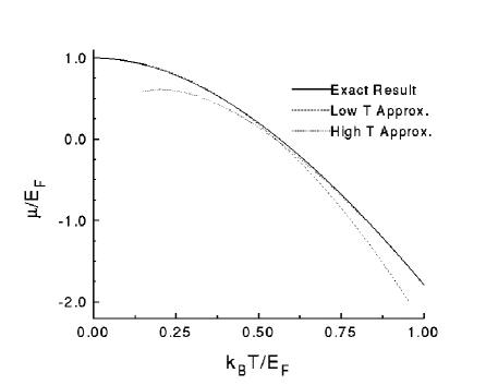
FIG. 1.: The chemical potential vs. temperature. Both axes are scaled by the Fermi energy, which results in a universal curve that applies to all harmonically trapped Fermi gases.

In eqs. (9) and (10), the particle number $N$ enters $\mu(T,N)$ only through the Fermi energy $E_{F}$. This result holds generally for all temperatures, as can be seen by casting eq. (4) in dimensionless form by scaling $E$, $\mu$, and $1/\beta$ by $E_{F}$. (The same conclusion holds for any density of states of the form $g(E)=AE^{b},$ for constant $A$, $b$.) Figure 1 is therefore a universal curve in the sense that it applies to harmonically trapped Fermi gases containing any number of particles.

The specific heat[10] per particle of the trapped Fermi gas, $1/N\;\partial U/\partial T|_{N}$, is shown in figure 2. It is a monotonic function of temperature. For low temperatures the specific heat per particle is $\pi^{2}k_{B}(k_{B}T/E_{F})$; at high temperatures $C=3Nk_{B}$, as we approach the equipartition limit for particles in a harmonic potential.

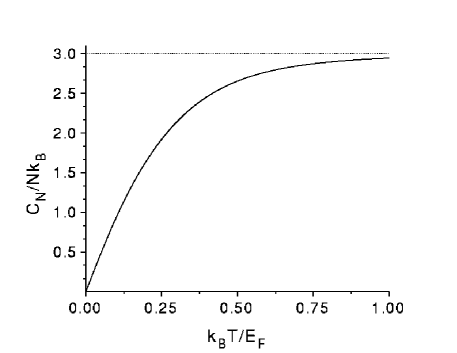
FIG. 2.: The heat capacity vs. temperature. The heat capacity is scaled by $k_{B}N$ and the temperature by $E_{F}$. The classical result is shown by the dotted line.

V Semiclassical (Thomas-Fermi) approximation

Since the exact eigenstates of the harmonic potential are well-known, the properties of a harmonically trapped ideal gas can in principle be found directly by summing over these states. It is useful, however, to have approximate forms for various observables that can be computed directly in the large $N$ limit, where the exact sums become unwieldy.

In the “semiclassical” or Thomas-Fermi approximation,[11] the state of each atom is labeled by a position ${\bf r}$ and a wavevector ${\bf k}$, which can be viewed as the centers of a wavepacket state. The energy of the particle is simply the corresponding value of the Hamiltonian; the density of states in the six-dimensional phase space $({\bf r},{\bf k})$ is $(2\pi)^{-3}$, where sums over states are replaced by integrals over phase space. These semiclassical approximations are valid in the limit of large $N$, as discussed in the Appendix.

In the semiclassical limit, the number density in phase space is

$$p({\bf r},{\bf k};T,\mu)=\frac{1}{(2\pi)^{3}}\frac{1}{e^{\beta({\cal H}({\bf r},\hbar{\bf k})-\mu)}+1}.$$ (11)

The chemical potential is given implicitly by the requirement

$$N=\int d^{3}{\bf r}\;d^{3}{\bf k}\ p({\bf r},{\bf k};T,\mu).$$ (12)

It follows from the correspondence principle that the Thomas-Fermi calculation of $\mu(T,N)$ using eq. (12) reproduces the exact result obtained from eq. (4); this is easily confirmed for the harmonic oscillator, since the two integrals are related by a simple change-of-variables.

After computing $\mu(T,N)$, it is straightforward to calculate the spatial and momentum distribution functions

$$n({\bf r};T) = \int d^{3}{\bf k}\ p({\bf r},{\bf k};T,\mu)$$ (13)

$$\tilde{n}({\bf k};T) = \int d^{3}{\bf r}\ p({\bf r},{\bf k};T,\mu).$$ (14)

VI Spatial distribution at zero temperature

At zero temperature, we may define a “local” Fermi wavenumber $k_{F}({\bf r})$ by

$$\frac{\hbar^{2}k_{F}({\bf r})^{2}}{2M}+V({\bf r})=E_{F},$$ (15)

where $V({\bf r})$ is the trap potential. The density $n({\bf r})$ is then simply the volume of the local Fermi sea in $k$-space, multiplied by the density of states $(2\pi)^{-3}$:

$$n({\bf r};T=0)=\frac{k_{F}({\bf r})^{3}}{6\pi^{2}}.$$ (16)

Note that $n({\bf r})$ vanishes for $\rho>R_{F}$, where $\rho$ is the effective distance

$$\rho\equiv[x^{2}+y^{2}+\lambda^{2}z^{2}]^{1/2}.$$ (17)

Combining eqs. (15) and (16), we find [6, 12]

$$n({\bf r};T=0)=\frac{N\lambda}{R_{F}^{3}}\frac{8}{\pi^{2}}[1-\frac{\rho^{2}}{R_{F}^{2}}]^{3/2}$$ (18)

for $\rho\leq R_{F}$. The cloud encompasses an ellipsoid with diameter $2R_{F}$ in the $xy$ plane, and diameter $2R_{F}/\lambda$ along the $z$ axis. This aspect ratio is the same as that of a classical gas in the same potential, since the Boltzmann distribution is proportional to $\exp[-M\omega^{2}\rho^{2}/2k_{B}T]$.

VII Momentum distribution at zero temperature

One way to characterize the state of a trapped gas is to allow a rapid adiabatic expansion and then measure the velocity distribution by time-of-flight spectroscopy.[1] For the degenerate Bose gas, the observed anisotropy of this velocity distribution is dramatic evidence for quantum statistical effects. The semiclassical momentum distribution for a degenerate Fermi gas at zero-temperature is simply

$$\tilde{n}({\bf k};T=0)=\frac{1}{(2\pi)^{3}}\int d^{3}{\bf r}\ \Theta(k_{F}({\bf r})-|{\bf k}|),$$ (19)

where $\Theta(k_{F}({\bf r})-|{\bf k}|)$ is the unit step function. The integral (19) is the real-space volume within which the local Fermi wavevector exceeds $|{\bf k}|$:

$$\tilde{n}({\bf k};T=0)=\frac{N}{K_{F}^{3}}\frac{8}{\pi^{2}}[1-\frac{|{\bf k}|^{2}}{K_{F}^{2}}]^{3/2},$$ (20)

where the maximum occupied wavenumber $K_{F}$ was defined in eq. (7). Note that $k_{F}({\bf r}=0)=$ $K_{F}$.

Despite the spatial anisotropy of the trap, the momentum distribution of the degenerate Fermi gas is isotropic. This isotropy is a general feature of trapped Fermi gases, independent of trap potential,[13] since from eq. (19) we see that $\tilde{n}({\bf k})$ depends only on the magnitude of ${\bf k}$.

The spatial and momentum distributions (18, 20) both have the same functional form, because ${\cal H}$ is a quadratic function of both position and momentum. In this sense, the distribution (18) can be viewed as a Fermi sea in real-space. The anisotropy of $n({\bf r})$ is due to the unequal spring constants, while the isotropy of $\tilde{n}({\bf k})$ is due to the isotropy of mass. That is, $p_{x}^{2}$, $p_{y}^{2},$ and $p_{z}^{2}$ enter the Hamiltonian with the same coefficient, while $x^{2},$ $y^{2},$ and $z^{2}$ need not.

VIII Numerical results

In the semiclassical approximation, the spatial and momentum distributions are easily determined numerically for any temperature as described in section V. As with the chemical potential, an appropriate scaling of these two distributions yields a universal form for all harmonically trapped Fermi gases when plotted vs. the scaled variables $\rho/R_{F}$ and $|{\bf k}|/K_{F}$, respectively.

Figure 3 shows the scaled density vs. scaled distance for $k_{B}T/E_{F}$ of 0, 0.25, 0.5, 0.75, and 1. At low temperatures, the density is close to their zero temperature form, with a thin evaporated “atmosphere” of thickness $\sim R_{F}(k_{B}T/E_{F})$ surrounding a degenerate liquid “core.”

In the classical limit, the density approaches a Gaussian in $\rho$, with a width given by the equipartition theorem: $\langle\rho^{2}\rangle=3R_{F}^{2}(k_{B}T/E_{F}).$ As shown in figure 3, this accurately describes the density distribution for $k_{B}T/E_{F}=1$. The evolution of the density profile from its low-temperature Fermi form (18) to the classical limit can be tracked by calculating the mean-square excursion $\langle\rho^{2}\rangle$, which is shown in figure 4 in the dimensionless form $\langle\rho^{2}\rangle/R_{F}^{2}$ vs. $k_{B}T/E_{F}$. This is again a universal curve for all harmonically trapped Fermi gases.

As noted above for zero temperature, the momentum distribution at non-zero temperature has the same form as the spatial distribution, since momentum and position both enter the single particle Hamiltonian quadratically. Thus the scaled momentum distribution $K_{F}^{3}\tilde{n}({\bf k})/N$ vs. $|{\bf k}|/K_{F}$ is also given by figure 3. Similarly, figure 4 illustrates the scaled mean-square momentum $\langle{\bf k}^{2}\rangle/K_{F}^{2}$ vs. $|{\bf k}|/K_{F}$ as well.

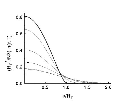
FIG. 3.: The universal spatial and momentum density distributions for $k_{B}T/E_{F}=0\$(bold),$\ 0.25$,$\ 0.5$,$\ 0.75$, and $1.0$. The classical result for $k_{B}T/E_{F}=1$ is shown as a dashed line.

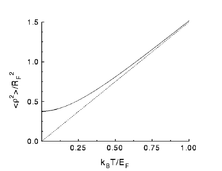
FIG. 4.: The mean-square variation of the size of the cloud interpolates between a low-temperature degenerate regime and a high-temperature limit that is well-described by the equipartition theorem.

IX Perturbations

What happens if the potential is not perfectly harmonic? We may treat $\delta V({\bf r})$ as a perturbation. Here we focus our attention on the $T=0$ case. From eq. (15), a change in trap potential shifts the local Fermi wavenumber by

$$\delta k_{F}({\bf r})=\frac{M}{\hbar k_{F}({\bf r})}[\delta E_{F}-\delta V({\bf r})],$$ (21)

where $\delta E_{F}$ is the change in Fermi energy. From eq. (16), the corresponding change in density is

$$\delta n({\bf r})=\frac{Mk_{F}({\bf r})}{2\pi^{2}\hbar}[\delta E_{F}-\delta V({\bf r})],$$ (22)

where the Fermi energy is adjusted to make $\int d^{3}{\bf r}\;\delta n({\bf r})$ vanish:

$$\delta E_{F}=\frac{\int d^{3}{\bf r}\delta V({\bf r})k_{F}({\bf r})}{\int d^{3}{\bf r}k_{F}({\bf r})}.$$ (23)

Interactions between particles (which are small for spin-aligned gases) can be treated as a perturbation $\delta V({\bf r})=Un({\bf r})$, where $U$ is a parameter related to the $p$-wave scattering length.

X Comparison with the Bose gas

The interacting Bose gases of refs. [1] and [2] are in the Thomas-Fermi regime[14]. Since the gases remain dilute, two-body scattering may be treated by a delta-function pseudopotential of strength $U=4\pi\hbar^{2}a/M$, where $a$ is the $s$-wave scattering length. When the dimensionless parameter $UN/\hbar\omega\lambda\sigma_{r}^{3}$ is large (as is appropriate for the experiments of refs. [1] and [2]) the density profile of the interacting Bose gas is [14]

$$n_{B}({\bf r})={{R_{B}^{2}}\over{2U}}\ \big{[}1-\frac{\rho^{2}}{R_{B}^{2}}\big{]},$$ (24)

with maximum radius

$$R_{B}=(\frac{15\lambda UN}{4\pi})^{1/5}.$$ (25)

Note that the characteristic radius scales more slowly with particle number for the Fermi gas ($N^{1/6}$) than for the interacting Bose gas ($N^{1/5}$); similarly, the Fermi energy scales as $N^{1/3}$ while the zero temperature chemical potential of the Bose gas varies more rapidly, as $N^{2/5}$.

The axial/radial aspect ratio for both classical and degenerate trapped gases is $\lambda$, since in every case the densities are functions of $\rho$ only. The velocity (momentum) distributions, however, can be quite different: for classical and Fermi gases the velocity distribution is isotropic, while $\tilde{n}({\bf k})$ for a zero temperature Bose gas is the square of the Fourier transform of $\sqrt{n_{B}({\bf r})}$. This is notably anisotropic. Note that as $N$ increases, both $R_{F}$ and $R_{B}$ increase, but the widths of the respective momentum distributions go in opposite directions: $K_{F}$ increases with $N$, while the typical momentum of a particle in a trapped Bose condensate decreases with particle number, since $K_{B}\sim 1/R_{B}$ by the uncertainty principle.

It is amusing to compare the interatomic repulsion in a Bose gas with the effective repulsion experienced by fermions due to the Pauli exclusion principle. Equating the characteristic Fermi and Bose radii (6, 25) we see that, crudely speaking, the spatial distribution of a degenerate Fermi gas is mimicked by that of a Bose gas interacting via an effective “Pauli pseudopotential” $U_{\rm eff}\sim E_{F}(R_{F}^{3}/N)$, which is the characteristic energy multiplied by the volume per particle. Equivalently, the effective scattering length brought about by the Pauli principle is $a_{\rm eff}\sim K_{F}^{-1}$, i.e., the inter-particle spacing. (This is quite expected, since the inter-particle spacing is the only appropriate length in the ideal Fermi gas.) The use of such an effective interaction is limited by the fact that (a) the momentum distributions of the Fermi and Bose gases remain quite different and (b) the gas is not dilute with respect to the exclusion-induced “interactions” since $K_{F}a_{\rm eff}$ is of order unity.

XI Acknowledgements

We thank Mark Kasevich, David Weiss, and Ike Silvera for useful and interesting discussions. This work was supported by the National Science Foundation under grant NSF-DMR-91-57414, and the Committee on Research at UC Berkeley. Work at Brandeis was supported by the Sloan Center for Theoretical Neurobiology.

XII Appendix: Validity of the semiclassical approximation

The semiclassical approximation can be safely applied to an inhomogeneous Fermi gas of density $n({\bf r})$ if we can imagine partitioning the system into cells of linear dimension ${\ell}$ such that the following two conditions are simultaneously met:

(1) The number of particles in a cell is much greater than unity, so that a local Fermi sea may be envisioned:

$$n(r){\ell}^{3}\gg 1.$$ (26)

(2) The variation of the trap potential across the cell (${\ell}\nabla V$) must be small compared with the local Fermi energy $\hbar^{2}k_{F}(r)^{2}/2M$, so that within a cell the potential energy is nearly constant. At low temperature, this condition becomes

$$\ell M\omega^{2}r\ll\frac{\hbar^{2}}{2M}[6\pi^{2}n(r)]^{2/3},$$ (27)

where we have used eq. (16).

Combining eqs. (26) and (27), we see that to be able to choose a (possibly $r$-dependent) cell size ${\ell}$ that simultaneously satisfies these two conditions, the number of particles per quantum volume must satisfy

$$n(r)\sigma^{3}\gg\frac{r}{\sigma},$$ (28)

where $\sigma$ is as before the quantum length $(\hbar/M\omega)^{1/2}$ and we have omitted factors of order unity.

At low temperatures, the semiclassical density given by eq. (18) scales as $N/R_{F}^{3}\sim N^{1/2}/\sigma^{3}$ near the origin, so the Thomas-Fermi approximation is always self-consistent at the center of the trap for large $N$. (This can be confirmed at ${\bf r}=0$ by direct summation of the squares of the simple harmonic oscillator eigenfunctions up to energy $E_{F}$.) Near the periphery of the cloud, however, the density becomes small, and the approximation is not valid. It is easy to show that semiclassical treatment fails within a shell at the periphery of the cloud, whose thickness $\delta R\sim$ $1/K_{F}\sim$ $\sigma N^{-1/6}$ vanishes in the limit of large $N$. Within this shell only the exponential tails of a few single particle states contribute to the density; this is analogous to the corresponding region of the Bose gas.[15]

REFERENCES

- [1] M.H. Anderson, J.R. Ensher, M.R. Matthews, C.E. Weiman, and E.A. Cornell, Science 269, 198 (1995).
- [2] K.B. Davis, M.O. Mewes, M.R. Andrews, N.J. van Druten, D.S. Durfee, D.M. Kurn, and W. Ketterle, Phys. Rev. Lett. 75, 3969 (1995).
- [3] C.C. Bradley, C.A. Sackett, J.J. Tollett, and R.G. Hulet, Phys. Rev. Lett. 75, 3969 (1995).
- [4] H.T.C. Stoof, M. Houbiers, C.A. Sackett, and R.G. Hulet, Phys. Rev. Lett., 76 10 (1996).
- [5] V.V. Goldman, I.F. Silvera, and A.J. Leggett, Phys. Rev. B 24, 2870 (1981).
- [6] I.F. Silvera and J.T.M. Walraven, J. Appl. Phys. 52, 2304 (1981).
- [7] D.A. Butts and D.S. Rokhsar, unpublished.
- [8] O.O. Tursunov and O.V. Zhirov, Phys. Lett. 222, 110 (1994).
- [9] B.L.G. Bakker, M.I. Polikarpov, and A.I. Veselov, quant-ph/9511009 (1995).
- [10] Note that the trapped gas does not occupy a container of externally fixed size, and so we do not introduce separate constant-volume and constant-pressure specific heats. As the gas is heated, it expands against the harmonic potential, doing work; the specific heat of the harmonically trapped system is therefore expected to be larger than that of a comparable gas-in-a-box at fixed volume. Since the harmonic restoring force grows linearly with the size of the cloud, the effective pressure it exerts will also vary.
- [11] L.H. Thomas, Proc. Cambridge Phil. Soc., 23, 542 (1927); E. Fermi, Z. Physik, 48, 73 (1928).
- [12] I.F. Silvera, Physica 109-110B, 1499 (1982).
- [13] A more familiar case is the ideal Fermi gas in a rectangular box – the spatial distribution is clearly anisotropic, but the momentum distribution isn’t, since the density of states in -space is uniformly .
- [14] G.Baym and C.J. Pethick, Phys. Rev. Lett. 76, 6 (1996).
- [15] S. Stringari, F. Dafolvo, and L. Pitaevski, preprint.