Quantum Physics and Computers

Abstract

Recent theoretical results confirm that quantum theory provides the possibility of new ways of performing efficient calculations. The most striking example is the factoring problem. It has recently been shown that computers that exploit quantum features could factor large composite integers. This task is believed to be out of reach of classical computers as soon as the number of digits in the number to factor exceeds a certain limit. The additional power of quantum computers comes from the possibility of employing a superposition of states, of following many distinct computation paths and of producing a final output that depends on the interference of all of them. This “quantum parallelism” outstrips by far any parallelism that can be thought of in classical computation and is responsible for the “exponential” speed-up of computation.

Experimentally, however, it will be extremely difficult to “decouple” a quantum computer from its environment. Noise fluctuations due to the outside world, no matter how little, are sufficient to drastically reduce the performance of these new computing devices. To control the nefarious effects of this environmental noise, one needs to implement efficient error–correcting techniques.

1 Computation and Physics

We are not used to thinking of computation in physical terms. We look on it as made up of theoretical, mathematical operations; but under close scrutiny, effecting a computation is essentially a physical process. Take a simple example, say “$2+3$”; how is this trivial computation handled by a computer? The inputs $2$ and $3$ are two abstract quantities, and before carrying out any computation, they are encoded in a physical system. This can take several radically different forms depending on the computing device: voltage potentials at the gates of a transistor on a silicon microchip, beads on the rods of an abacus, nerve impulses on the synapse of a neuron, etc. The computation itself consists of a set of instructions (referred to as an algorithm) carried out by means of a physical process. Completion of the algorithm yields a result that can be reinterpreted in abstract terms: we observe the physical system (for instance, by looking at the display of a calculator) and conclude that the result is $5$. The crucial point here is that, although $2+3$ may be defined abstractly, the process that enables us to conclude that $2+3$ equals $5$ is purely physical.

The theory of computation has been long considered a completely theoretical field, detached from physics. Nevertheless, pioneers such as Turing, Church, Post and Gödel were able, by intuition alone, to capture the correct physical picture, but since their work did not refer explicitly to physics, it has been for a long time falsely assumed that the foundations of the theory of classical computation were self–evident and purely abstract. Only in the last two decades were questions about the physics of computation asked and consistently answered [1]. These later developments led to a complete and thorough understanding of the physical limits of classical computers; but they were concerned only with the classical theory of computation, for which the computing device is supposed to obey the laws of classical physics. This is fine as long as one asks questions about computers we have now: any computer that was ever built, from the oldest abacus to the latest supercomputer, behaves indeed in a classical fashion; but we live in a quantum world and quantum objects tend to behave quite differently from classical ones. So what about quantum… computers?

Despite early suggestions that “something new” may exist when computers are enabled to behave in a quantum mechanical way, it was not until the seminal work of Deutsch in 1985 [2] that the foundations of quantum computation were laid and properly formalised. In his article, Deutsch considers the situation where computers behave like quantum systems and can enter highly non–classical states. These quantum computers could, for instance, exist in a superposition of states. Each state could follow coherently a distinct computational path and interfer to produce a final output. This “quantum parallelism”, achieved in a single piece of hardware, outstrips by far any parallelism that can be thought of in classical computers, thus potentially providing quantum computers with unprecedented power. It took indeed another decade to gain clear evidence of the power of quantum computers and to exhibit specific problems that were intractable on classical computers but that could be solved efficiently on a quantum one. The most striking example is the factorisation problem. Shor [3] has shown recently that using a quantum algorithm (i.e. an algorithm that runs on a quantum computer) it is possible to factor large integers efficiently.

Factorisation is believed to be intractable (or at best extrememly difficult and time–consuming) on any classical computer, and Shor’s algorithm shows for the first time that the class of problems accessible to quantum computers includes problems that (so far) cannot be handled efficiently by classical devices. In fact factorisation is not of purely academic interest only: it is the problem which underpins the security of many classical public key cryptosystems. For example, RSA [4], the most popular public key cryptosystem (named after the three inventors, Rivest, Shamir, and Adleman), gets its security from the difficulty of factoring large numbers. Hence for the purpose of cryptoanalysis the experimental realisation of quantum computation is a most interesting issue. This growing interest in the field during these last years is backed up by the enormous experimental progress made in testing fundamentals of quantum mechanics. In the last decade or two, it has become possible to isolate and study single microscopic quantum systems, giving new insights into the meaning of quantum mechanics, opening new horizons of research and above all giving the possibility to test fundamental ideas such as those involved in quantum computation.

This paper is organised as follows. Section 2 is concerned with the limits of classical computation. In section 3, I introduce the basic notions and tools of quantum computation necessary to understand the factorisation algorithm presented in section 4. Section 5 deals with possible ways of assembling a quantum computer out of basic elements, while experimental realisations are presented in section 6, together with some fundamental limitations imposed by the difficulty of isolating a quantum system from its environment. The final section gives some conclusions and discusses future prospects in the field.

2 A Brief Look at Classical Complexity

Setting benchmarks is a useful process to understand in which sense quantum algorithms outperform classical ones. There are rigorous ways of defining what makes an algorithm efficient for solving a particular problem [5]. For instance we can ask questions such as “how does the memory or the time of a computation increase with the size of the input of the problem ?” We generally take the input size to be the amount of information (measured in bits) needed to specify the input. For example, a number $N$ requires $\sim\log_{2}(N)$ bits of storage on a computer (up to a fixed multiplicative factor ($\log_{2}(10)$), the size is the number of digits of $N$ in a decimal system).

As an illustration, let us look at how the time needed to solve two related problems varies with the size of the input. On one hand consider the problem of factoring a number $N$ of size $L$ (i.e. $L$ digits). Factoring $N$ means finding its prime factors i.e. finding the set of integer numbers $\{p_{i}\}$ such that any $p_{i}$ in that set divides $N$ with the remainder $0$. One way to calculate the prime factors is to try to divide $N$ by $2,3,\ldots\sqrt{N}$ and to check the remainder. This method is very time consuming. It requires about $\sqrt{N}\approx 10^{L/2}$ divisions, hence the time it takes to execute this algorithm increases exponentially with $L$. An as yet hypothetical computer that can perform as many as $10^{10}$ divisions per second would take about a second to factor a $20$ digit number, about a year to factor a $34$ digit number and more than the estimated age of the Universe ($10^{17}s$) to factor a $60$ digit long number.

The related problem of multiplying two $L$ digit–long numbers together can be solved much faster. The algorithm we are taught in school (reducing the complete multiplication in single digit multiplications) requires $L^{2}$ of these basic operations. Multiplying two $60$ digits numbers would then take only a blink of an eye on the hypothetical computer (see Fig. 1).

Figure 1: a) Asymptotic behaviour (on the hypothetical computer) of the completion time (as a function of the input size) for two related problems. For the factorisation problem the time grows exponentially (dashed line), but for multiplication it only grows polynomially (plain line). b) Even when the order of the exponential is small ($t\sim e^{\epsilon t}$, with $0<\epsilon\ll 1$, $\epsilon=0.1$ in the figure) and the degree of the polynomial is large ($t\sim t^{\eta}$ with $\eta\gg 1$, $\eta=10$ in the figure) the two curves will cross and above a given input size the exponential case will become very inefficient. From the point of view of complexity, only the distinction between polynomial and exponential behaviour matters.

For both problems, the algorithms presented are not the most efficient: for factorisation the best algorithm is subexponential and requires $\simeq e^{(L^{1/3}(\log L)^{2/3})}$ operations [6], and for multiplication $L\log(L)\log(\log(L))$, in the limit that the numbers we multiply are very large (more than several hundred digits) [7]. Even with these algorithms this asymmetry between the two problems remains: one problem is solved in a time that grows (sub)exponentially with the size of the input (i.e. with the number of digits of the input), the other requires a time that grows only polynomially (cf Fig. 1b). This asymmetry is a clear illustration of how different problems may require a very different amount of resources (in this case time) for obtaining the solution to a problem.

Problems for which the best algorithm runs polynomially (e.g. multiplication) are said to be tractable and belong to what mathematicians have called the complexity class P, whereas, when the time grows exponentially (e.g. factorisation), they are said to be intractable, and belong to other classes of complexity (NP, EXP, depending on other characteristics of the problem [5]). The strength of this classification is that it does not depend on the physical realisation of the computer as long as the computer obeys the laws of classical physics. Mathematicians have shown that, as long as a computer behaves classically, it is strictly equivalent to a toy model called a Turing Machine. As practical devices, Turing Machines probably epitomise the worst nightmare of programmers and computer scientists, but they are an invaluable tool used by mathematicians to define and establish complexity classes.

By showing that Turing Machines that obey the laws of quantum mechanics could support new types of algorithms (quantum algorithms) Deutsch was able to define new complexity classes and establish a new hierarchy [2]. However, it was not recognised until recently that the class of problems that can be solved in polynomial time with a quantum algorithm (the class QP) includes problems for which the best classical algorithm runs exponentially. Factorisation is one of those, but before explaining how quantum computers tackle this task, let me introduce some basic definitions.

3 Quantum bits and pieces

3.1 Bits and Registers

At the heart of a quantum computer lies the quantum bit [8] or simply qubit as the natural extension of the classical notion of bit. Instead of a simple two–state system that can either be in state $0$ or $1$, a qubit is a quantum two–level system, that in addition of the two eigenstate $|0\rangle$ and $|1\rangle$ (the labels are here a mere convention, but correspond usually to the ground and excited state of the two–level system) can be set in any superposition of the form

$$\mbox{$|\psi\rangle$}=c_{0}\mbox{$|0\rangle$}+c_{1}\mbox{$|1\rangle$}.$$ (1)

Any quantum two–level system is a potential candidate for a qubit, but to help to construct a mental picture, it is a good idea to carry a concrete, albeit somehow idealised, physical example of a qubit. In the following it will be useful to think of a qubit as a spin–$1/2$ particle. $|0\rangle$ and $|1\rangle$ will correspond respectively to the spin–down and spin–up eigenstates (along a prearranged axis of quantisation, usually set by an external constant magnetic field).

Although a qubit can be prepared in an infinite number of different quantum states (by choosing different complex coefficient $c_{i}$’s in Eq. (1)) it cannot be used to transmit more than one bit of information. This is because no detection process can reliably differentiate between nonorthogonal states [9]. However, qubits (and more generally information encoded in quantum systems) can be used in systems developed for quantum cryptography [10], quantum teleportation [11] or quantum dense coding [12]. The problem of measuring a quantum system is a central one in quantum theory, and much attention has been and is still devoted to this subject [13]. In a classical computer, it is possible in principle to inquire at any time (and without disturbing the computer) about the state of any bit in the memory. In a quantum computer, the situation is different. Qubits can be in superposed states, or can even be entangled with each other, and the mere act of measuring the quantum computer alters its state. Performing a measurement on a qubit in a state given by Eq. (1) will return $0$ with probability $|c_{0}|^{2}$ and $1$ with probability $|c_{1}|^{2}$; but more importantly, the state of the qubit after the measurement (post–measurement state) will be $|0\rangle$ or $|1\rangle$ (depending on the outcome), and not $c_{0}\mbox{$|0\rangle$}+c_{1}\mbox{$|1\rangle$}$. With our spins, it is convenient to think of the measuring apparatus as a Stern–Gerlach device into which the qubits are sent when we want to measure them. When measuring a state of the form of Eq. (1), outcomes $0$ and $1$ will be recorded with a probability $|c_{0}|^{2}$ and $|c_{1}|^{2}$ on the respective detector plate (see Fig. 2).

We will call a collection of qubits a quantum register, or simply a register. As in the classical case, it can be used to encode more complicated information. For instance, the binary form of $6$ is $110$ and loading a quantum register with this value is done by preparing three qubits in state $|1\rangle\otimes|1\rangle\otimes|0\rangle$. In the following, we use a more compact notation: $|a\rangle$ stands for the direct product $|a_{n-1}\rangle\otimes|a_{n-2}\rangle\ldots|a_{1}\rangle\otimes|a_{0}\rangle$ which denotes a quantum register prepared with the value $a=2^{0}a_{0}+2^{1}a_{1}+\ldots 2^{n-1}a_{n-1}$. Two states $|a\rangle$ and $|b\rangle$ are orthogonal as soon as $a\neq b$:

$$\mbox{$\langle{{a}}\mathrel{|{\vphantom{{a}{b}}}\kern-1.2pt}{{b}}\rangle$}=\mbox{$\langle{{a_{0}}}\mathrel{|{\vphantom{{a_{0}}{b_{0}}}}\kern-1.2pt}{{b_{0}}}\rangle$}\mbox{$\langle{{a_{1}}}\mathrel{|{\vphantom{{a_{1}}{b_{1}}}}\kern-1.2pt}{{b_{1}}}\rangle$}\ldots\mbox{$\langle{{a_{n-1}}}\mathrel{|{\vphantom{{a_{n-1}}{b_{n-1}}}}\kern-1.2pt}{{b_{n-1}}}\rangle$},$$ (2)

and if $a\neq b$ at least one of the terms in the r.h.s of the above expression is zero so that $\mbox{$\langle{{a}}\mathrel{|{\vphantom{{a}{b}}}\kern-1.2pt}{{b}}\rangle$}=0$.

For an $n$–bit register, the most general state can be written as

$$\mbox{$|\Psi\rangle$}=\sum_{x=0}^{2^{n}-1}c_{x}\mbox{$|x\rangle$}.$$ (3)

Note that this state describes the situation in which several different values of the register are present simultaneously; just as in the case of the qubit, there is no classical counterpart to this situation, and there is no way to gain a complete knowledge of the state of a register through a single measurement.

With our spin picture in mind, measuring the state of a register is done by passing one by one the various spins that form the register in a Stern–Gerlach apparatus and record the results (Fig. 2). For instance a two–bit register initially prepared in the state $\mbox{$|\psi\rangle$}=1/\sqrt{2}(\mbox{$|0\rangle$}+\mbox{$|3\rangle$})$, i.e. $1/\sqrt{2}(\mbox{$|0\rangle$}\mbox{$|0\rangle$}+\mbox{$|1\rangle$}\mbox{$|1\rangle$})$, will with equal probability result in either two successive clicks in the up–detector or two successive clicks in the the down–detector. The post–measurement state will be either $|0\rangle$ or $|3\rangle$, depending on the outcome. A record of a click–up followed by a click–down, or the opposite (click–down followed by click–up), signals an experimental or a preparation error, because neither $\mbox{$|2\rangle$}=\mbox{$|1\rangle$}\mbox{$|0\rangle$}$ nor $\mbox{$|1\rangle$}=\mbox{$|0\rangle$}\mbox{$|1\rangle$}$ appear in $|\psi\rangle$.

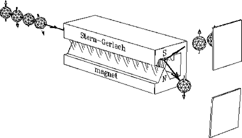
Figure 2: An idealised measuring device for a quantum computer. Registers made out of spins, each one in a random state, pass through a Stern–Gerlach magnet that performs a measurement in the spin–up spin–down basis (i.e. the basis $|0\rangle$ and $|1\rangle$). The spins are deflected by the device and detected by the detector (plates). After passing through the device, the spins point no longer randomly, but are in one of the two possible eigenstates.

3.2 Gates

In a classical computer, the processing of information is done by logic gates. A logic gate maps the state of its input bits into another state according to a truth table. The simplest non–trivial classical gate is the NOT gate, a one–bit gate which negates the state of the input bit: $0$ becomes $1$ and vice–versa. The corresponding quantum gate is implemented via a unitary operation that evolves the basis states into the corresponding states according to the same truth table. For instance the quantum version of the classical NOT is the unitary operation $U_{{\mbox{$\mbox{\scriptsize\sf NOT}$}}}$ such

$$\begin{array}[]{l}U_{{\mbox{$\mbox{\scriptsize\sf NOT}$}}}\mbox{$|0\rangle$}=\mbox{$|1\rangle$}\\ U_{{\mbox{$\mbox{\scriptsize\sf NOT}$}}}\mbox{$|1\rangle$}=\mbox{$|0\rangle$}.\end{array}$$ (4)

In quantum mechanics, the notion of gate can be extended to operations that have no classical counterpart. For instance, the operation $U_{{\mbox{$\mbox{\scriptsize\sf A}$}}}$ that evolves

$$\begin{array}[]{l}U_{{\mbox{$\mbox{\scriptsize\sf A}$}}}\mbox{$|0\rangle$}={1}/{\sqrt{2}}\;(\mbox{$|0\rangle$}+\mbox{$|1\rangle$})\\ U_{{\mbox{$\mbox{\scriptsize\sf A}$}}}\mbox{$|1\rangle$}={1}/{\sqrt{2}}\;(\mbox{$|0\rangle$}-\mbox{$|1\rangle$}),\end{array}$$ (5)

defines a perfectly “legal” quantum gate. Note that it evolves “classical” states into superpositions and therefore cannot be regarded as classical. This gate is of great utility: take an $n$–bit quantum register initially in the state $|0\rangle$ and apply to every single qubit of the register the gate $U_{{\mbox{$\mbox{\scriptsize\sf A}$}}}$. The resulting state is

$$\begin{array}[]{rl}\mbox{$|\psi\rangle$}&=U_{{\mbox{$\mbox{\scriptsize\sf A}$}}}\otimes U_{{\mbox{$\mbox{\scriptsize\sf A}$}}}\otimes\ldots U_{{\mbox{$\mbox{\scriptsize\sf A}$}}}\mbox{$|00\ldots 0\rangle$}\\ &=\frac{1}{\sqrt{2}}(\mbox{$|0\rangle$}+\mbox{$|1\rangle$})\otimes\frac{1}{\sqrt{2}}(\mbox{$|0\rangle$}+\mbox{$|1\rangle$})\otimes\ldots\frac{1}{\sqrt{2}}(\mbox{$|0\rangle$}+\mbox{$|1\rangle$})\\ &=\frac{1}{2^{n/2}}(\mbox{$|00\ldots 0\rangle$}+\mbox{$|00\ldots 1\rangle$}+\ldots\mbox{$|11\ldots 1\rangle$})\\ &=\frac{1}{2^{n/2}}\sum_{x=0}^{2^{n}-1}\mbox{$|x\rangle$}.\end{array}$$ (6)

Thus, with a linear number of operations (i.e. $n$ application of $U_{{\mbox{$\mbox{\scriptsize\sf A}$}}}$) we have generated a register state that contains an exponential ($2^{n}$) number of distinct terms. It is quite remarkable that using quantum registers, $n$ elementary operations can generate a state containing all $2^{n}$ possible numerical values of the register. In contrast, in classical registers $n$ elementary operations can only prepare one state of the register representing one specific number. It is this ability of creating quantum superpositions which makes the “quantum parallel processing” possible. If after preparing the register in a coherent superposition of several numbers all subsequent computational operations are unitary and linear (i.e. preserve the superpositions of states) then with each computational step the computation is performed simultaneously on all the numbers present in the superposition.

3.3 Functions

Let me next describe now how quantum computers deal with functions. Consider a function

$$f:\,\{0,1,...\,2^{m}-1\}\longrightarrow\{0,1,...\,2^{n}-1\},$$ (7)

where $m$ and $n$ are positive integers. A classical device computes $f$ by evolving each labeled input, $0,1,...\,2^{m}-1$ into its respective labeled output $f(0),f(1),...\,f(2^{m}-1)$. Quantum computers, due to the unitary (and therefore reversible) nature of their evolution, compute functions in a slightly different way. Indeed, it is not directly possible to compute a function $f$ by a unitary operation that evolves $|x\rangle$ into $|f(x)\rangle$: if $f$ is not a one–to–one mapping (i.e. if $f(x)=f(y)$ for some $x\neq y$), then two orthogonal kets $|x\rangle$ and $|y\rangle$ can be evolved into the same ket $\mbox{$|f(x)\rangle$}=\mbox{$|f(y)\rangle$}$, thus violating unitarity. One way to compute functions which are not one–to–one mappings, while preserving the reversibility of computation, is by keeping the record of the input. To achieve this, a quantum computer uses two registers: the first register to store the input data, the second one for the output data. Each possible input $x$ is represented by $|x\rangle$, the quantum state of the first register. Analogously, each possible output $y=f(x)$ is represented by $|y\rangle$, the quantum state of the second register. States corresponding to different inputs and different outputs are orthogonal, $\langle x|x^{\prime}\rangle=\delta_{xx^{\prime}}$, $\langle y|y^{\prime}\rangle=\delta_{yy^{\prime}}$. The function evaluation is then determined by a unitary evolution operator $U_{f}$ that acts on both registers:

$$U_{f}\mbox{$|x\rangle$}\mbox{$|0\rangle$}=\mbox{$|x\rangle$}\mbox{$|f(x)\rangle$}.$$ (8)

It has been shown that as far as computational complexity is concerned, a reversible function evaluation, i.e. the one that keeps track of the input, is as good as a regular, irreversible evaluation [22]. This means that if a given function can be computed in polynomial time, it can also be computed in polynomial time using a reversible computation.

The computations we are considering here are not only reversible but also quantum, and we can do much more than computing values of $f(x)$ one by one. We can prepare a superposition of all input values as a single state and by running the computation $U_{f}$ only once, we can compute all of the $2^{m}$ values $f(0),\ldots,f(2^{m}-1)$,

$$\mbox{$|\psi\rangle$}=U_{f}\left(\frac{1}{2^{m/2}}\sum_{x=0}^{2^{m}-1}\mbox{$|x\rangle$}\right)\mbox{$|0\rangle$}=\frac{1}{2^{m/2}}\sum_{x=0}^{2^{m}-1}\mbox{$|x\rangle$}\mbox{$|f(x)\rangle$}.$$ (9)

It looks too good to be true so where is the catch? How much information about $f$ does the state $|\psi\rangle$ contain?

As we would expect, no quantum measurement can extract all of the $2^{m}$ values $f(0),f(1),\ldots,f(2^{m}-1)$ from $|\psi\rangle$. Imagine, for instance, performing a measurement on the first register of $|\psi\rangle$. Quantum mechanics enables us to infer several facts:

• Since each value $x$ appears with the same complex amplitude in the first register of state $|\psi\rangle$, the outcome of the measurement is equiprobable and can be any value ranging from $0$ to $2^{m}-1$.

• Assuming that the result of the measurement is $|j\rangle$, the post–measurement state of the two registers (i.e. the state of the registers after the measurement) is $\mbox{$|\tilde{\psi}\rangle$}=\mbox{$|j\rangle$}\mbox{$|f(j)\rangle$}$. Thus a subsequent measurement on the second register would yield with certainty the result $f(j)$, and no additional information about $f$ can be gained.

However, there are more subtle measurements that provide us with information about joint properties of all the output values $f(x)$ such as, for example, the periodicity of $f$. I will describe in the following sections how an efficient periodicity estimate can lead to a fast factorisation algorithm. But let me first introduce some mathematical results in number theory that are relevant to the problem. I shall not attempt to give a rigorous exposition nor to provide proofs, as they can be found in most textbooks on the subject (see for example [14]).

4 Quantum Factorisation

4.1 Periodic functions

The factorisation problem can be related to finding periods of certain functions. In particular one can show [15] that finding factors of $N$ is equivalent to finding the period of the function

$$f_{a,N}(x)=a^{x}\bmod N$$ (10)

where $a$ is any randomly chosen number which is coprime with $N$, i.e. which has no common factors with $N$ (if $a$ is not coprime with $N$, then the factors of $N$ are trivially found by computing the greatest common divisor of $a$ and $N$). This function gives the remainder after the division of $a^{x}$ by $N$. The function is periodic with period $r$ [14], which depends on $a$ and $N$.

Knowing the period $r$ of $f_{a,N}$, we can factor $N$ provided $r$ is even and $r\bmod N\neq-1$. When $a$ is chosen randomly the two conditions are satisfied with probability greater than $1/2$. The factors of $N$ are then given by $\gcd(a^{r/2}\pm 1,N)$, the greatest common divisor of $a^{r/2}\pm 1$ and $N$. Fortunately, for this last calculation, an easy and very efficient algorithm has been known since 300 BC. The algorithm, known as the Euclidean algorithm, runs in polynomial time on a classical computer, reducing thus the problem of factoring big numbers to the related task of finding the period of a function.

To see how this method works, let me illustrate it with a very simple example. Let us try to factor $N=15$. Firstly we select $a$, such that $\gcd(a,N)=1$, for instance $a=7$ (with $N=15$, $a$ could be any number from the set $\{2,4,7,8,11,13,14\}$). The values of $f_{7,15}(x)=7^{x}\bmod 15$ for $x=1,2,3,4,5,6,7\ldots$ are $1,7,4,13,1,7,4\ldots$ respectively and clearly the period here is $r=4$. $a^{r/2}$ gives $49$ and by computing the largest common divisors $\gcd(a^{r/2}\pm 1,N)$, we find the two factors of $15$: $\gcd(48,15)=3$ and $\gcd(50,15)=5$. The periods of $f_{a,15}(x)$ for other values $a$ in the set $\{2,4,7,8,11,13,14\}$ are respectively $\{4,2,4,4,2,4,2\}$ and in this particular example any choice of $a$ except $a=14$ leads to the correct result. For $a=14$ we obtain $r=2$, $a^{r/2}\equiv-1\bmod 15$ and the method fails.

Every step of this method, except finding $r$, can be performed in polynomial time on a classical computer. Unfortunately, finding $r$ is actually as time consuming as finding factors of $N$ by the trial division method since it requires us to evaluate $f_{a,N}(x)$ an number of times exponential in $L$ on average (where $L$ is the size of the number we want to factor, $L\simeq\log_{2}(N)$); however, if we employ quantum computation, $r$ can be evaluated very efficiently. Shor [3] describes a quantum algorithm which provides the period $r$ of a function and which runs efficiently (i.e. in polynomial time) on a quantum computer. Let me now outline the main features of this algorithm.

4.2 Using quantum parallelism for factorisation.

As was pointed out in Sect. 3.3, quantum mechanics enables us to compute a function $f$ for different values by just applying the corresponding unitary operator $U_{f}$ on a register previously set in a superposition of orthogonal states. Let us play this game for the function $f_{a,N}(x)$. Since the result cannot be larger than $N$, the output register, as defined in Sect. 3.3, should have at least $L$ qubits. For reasons that will become clear later, we will consider an input register of $2L$ bits. Both registers are initially loaded with the value $0$ and the total initial state is

$$\mbox{$|0\rangle$}\mbox{$|0\rangle$}.$$ (11)

We first set the input register into an equally weighted superposition of all possible states, from $0$ to $2^{2L}-1$ ($\simeq N^{2}$), by applying the gate $U_{{\mbox{$\mbox{\scriptsize\sf A}$}}}$ (defined in Sect. 3.2) on each qubit of the input register

$$\frac{1}{2^{L}}\sum_{x=0}^{2^{2L}-1}\mbox{$|x\rangle$}\mbox{$|0\rangle$}.$$ (12)

Applying the operator $U_{f_{a,N}}$ to this state, we obtain

$$\frac{1}{2^{L}}\sum_{x=0}^{2^{2L}-1}\mbox{$|x\rangle$}\mbox{$|f_{a,N}(x)\rangle$}.$$ (13)

At this stage, all the possible values of $f_{a,N}$ are encoded in the state of the second register, but as was pointed out earlier, they are not all accessible at the same time. On the other hand, we are not interested in the values themselves but only in the periodicity of the function. Let me proceed now with an example to see how this periodicity can be efficiently retrieved.

Taking the same values as in the example of the previous section ($N=15$ and $a=7$), the state of the two registers after applying $U_{f_{7,15}}$ is

$$\frac{1}{64}\left(\mbox{$|0\rangle$}\mbox{$|1\rangle$}+\mbox{$|1\rangle$}\mbox{$|7\rangle$}+\mbox{$|2\rangle$}\mbox{$|4\rangle$}+\mbox{$|3\rangle$}\mbox{$|13\rangle$}+\mbox{$|4\rangle$}\mbox{$|1\rangle$}+\mbox{$|5\rangle$}\mbox{$|7\rangle$}+\mbox{$|6\rangle$}\mbox{$|4\rangle$}+\mbox{$|7\rangle$}\mbox{$|13\rangle$}+\ldots\right),$$ (14)

At this point, we perform a measurement on the second register. We take each spin that forms the second register, pass it through our Stern–Gerlach measurement apparatus, record each outcome ($0$ or $1$) and reconstruct the value of the register. In Eq. (14), the second register encodes only the four different values $1,4,7$ or $13$, and therefore any other measurement outcome is impossible, unless an experimental error has occured. The state of the second register after a measurement with outcome $j$ is $|j\rangle$. For the first register the situation is a bit more delicate and the post–measurement state of the first register will be an equally weighted superposition of the states in Eq. (14) for which the second register was in state $|j\rangle$. Table 1 sums up the possible outcomes and the post–measurement states of the two registers.

$$\begin{array}[]{c|l|c}\mbox{outcome}&\hfill\mbox{post--measurement state}\hfill&\mbox{offset $l$}\\ \hline\cr\hline\cr\vspace{-2mm}\hfil\\ 1&\xi(\mbox{$|0\rangle$}+\mbox{$|4\rangle$}+\mbox{$|8\rangle$}+\;\>\ldots)\mbox{$|1\rangle$}&0\\ 4&\xi(\mbox{$|3\rangle$}+\mbox{$|7\rangle$}+\mbox{$|11\rangle$}+\ldots)\mbox{$|4\rangle$}&3\\ 7&\xi(\mbox{$|1\rangle$}+\mbox{$|5\rangle$}+\mbox{$|9\rangle$}+\;\>\ldots)\mbox{$|7\rangle$}&1\\ 13&\xi(\mbox{$|2\rangle$}+\mbox{$|6\rangle$}+\mbox{$|10\rangle$}+\ldots)\mbox{$|13\rangle$}&2\\ \end{array}$$

Table 1: Possible outcomes of the measurement performed on the second register of the state of the form $\frac{1}{2^{L}}\sum_{x=0}^{2^{2L}-1}\mbox{$|x\rangle$}\mbox{$|f_{a,N}(x)\rangle$}$, with $a=4$ and $N=15$. The post–measurement state and the offset $l$ is also given for each possible outcome.

We forget now about the second register and focus only on the state of the first one.

Let me dream for a while and imagine that quantum mechanics enables me to dictate the outcome of the measurement I perform on the second register. Imagine that I decide always to obtain, say, $4$. In this case, I would be able to prepare at will the quantum computer in the state

$$\xi(\mbox{$|3\rangle$}+\mbox{$|7\rangle$}+\mbox{$|11\rangle$}+\ldots)\mbox{$|4\rangle$}.$$ (15)

Returning to normal rules of quantum mechanics, I could now perform a measurement on the first register and obtain with equal probability any of the values $3,7,11,15\ldots$ etc. Repeating the procedure from the beginning two more times, I could, with a very high probability obtain two other distinct values, which would enable me to find the period very easily: if in these three successive runs, I obtain for instance $19$, $3$ and $11$, the period is easily found to be $\gcd(19-11,11-3)=4$.

Unfortunately, dictating the result of a measurement on the second register violates the rules of quantum mechanics. Measurement outcomes are probabilistic, and in my example, each allowed outcome ($1,4,7$ or $13$) is equiprobable. In this particular case, I could repeat the experiment a few times and retain only the runs for which the outcome is $4$. However, the notion of efficiency is defined for asymptotic behaviour and not for particular cases. The real question is to know how this technique will perform for increasing $N$’s. Quite clearly, it does not look promising; in a general case, when the period is $r$, there are $r$ possible different outcomes. Since $r$ also grows exponentially with $L$ (the size of $N$), the approach that consists of repeating the quantum computation over and over again until measuring in the second register at least three times the same value (in order then to perform a measurement on the first register and find the factor via a greatest common divisor calculation) is inefficient.

An additional ingredient is needed to make the quantum algorithm polynomially efficient. Whatever the outcome of the measurement was, the first register is left in an equally weighted superposition of the form

$$\mbox{$|\psi\rangle$}=\xi\sum_{j=0}^{\lfloor 2^{2L}/r\rfloor}\mbox{$|jr+l\rangle$},$$ (16)

with $r$ being the period of $f_{a,N}(x)$, $l$ an offset value and $\xi$ an appropriate normalisation factor. (cf. Fig. 3a and Table 1). Regardless of the outcome of the measurement, the period $r$ of the function $f_{a,N}$ is always reflected in the post–measurement state of the first register. But it is not readily accessible, as the offset $l$ depends probabilistically on the outcome of the measurement. It is nevertheless possible to get rid of this irritating offset by using a quantum equivalent of the classical Fast Fourier Transform. This operation is known as the Discrete Fourier Transform (DFT).

4.3 Discrete Fourier Transform

Consider the unitary operation $U_{{\mbox{$\mbox{\scriptsize\sf DFT}$}}}$ that acts on a quantum register and effects

$$U_{{\mbox{$\mbox{\scriptsize\sf DFT}$}}}\mbox{$|x\rangle$}=\frac{1}{2^{L}}\sum_{y}^{2^{2L}-1}\exp(2\pi i\frac{xy}{2^{2L}})\mbox{$|y\rangle$},$$ (17)

where $2L$ is the size of the register. The reason for calling this particular unitary transformation the discrete Fourier transform becomes obvious when we notice that in the transformation

$$U_{{\mbox{$\mbox{\scriptsize\sf DFT}$}}}\sum_{x=0}^{2^{2L}-1}c_{x}\mbox{$|x\rangle$}=\sum_{y}c_{y}\mbox{$|y\rangle$}$$ (18)

the coefficients $c_{y}$ are the discrete Fourier transforms of $c_{x}$’s i.e.

$$c_{y}=\frac{1}{2^{L}}\sum_{x=0}^{2^{2L}-1}\exp(2\pi i\frac{xy}{2^{2L}})c_{x}.$$ (19)

The strength of the DFT lies in the fact that when it acts on a periodic state of the form of Eq. (16), it will wipe out the offset $l$, and transform it into a phase factor that does not affect the probabilistic outcome of a later measurement on the register. Appendix A shows how the DFT on a $2L$–bit register maps a state of period $r$ into a state of period $2^{2L}/r$. When $r$ divides exactly $2^{2L}$, the resulting state has a nice closed form (cf. Fig. 3):

$$\mbox{$|\phi_{out}\rangle$}=\frac{1}{\sqrt{r}}\sum_{j=0}^{r-1}\exp(2\pi ilj/r)\;\mbox{$|j2^{2L}/r\rangle$}.$$ (20)

A more careful analysis is required when $r$ does not divide $2^{2L}$ (see Appendix A). Even in this more general case, the DFT retains the features illustrated in the particular situation above: it “inverts” the periodicity of the input ($r\rightarrow 2^{2L}/r$) and it has this translation invariance property which washes out the offset $l$ (Fig. 3b). Thus, by effecting $U_{{\mbox{$\mbox{\scriptsize\sf DFT}$}}}$ on states of the form of Eq. (16) with different $l$, we always end up with a state for which neither the outcome of a measurement, nor its probability depend on $l$ anymore.

In the previous section, I showed how to construct a state of a register with a periodic superposition and an arbitrary offset. Combining this method with a DFT, it is now possible to retrieve efficiently the “inverted” period $2^{2L}/r$ (cf. Fig. 3), from it the period $r$, and finally the factors of $N$.

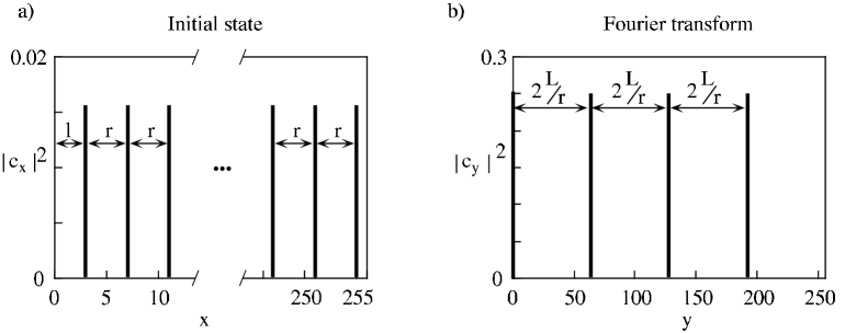
Figure 3: The DFT on an input state of the form $\sum_{x}c_{x}\mbox{$|x\rangle$}$ results in $\sum_{y}c_{y}\mbox{$|y\rangle$}$. When the input state is periodic, as in (a), the effect of the DFT is to eliminate the eventual offset $l$ and to invert the period $r\rightarrow 2^{L}/r$ (b). In the figure $L=8$, $l=3$ and $r=4$. In this particular case the period $r$ divides exactly $2^{L}$, resulting thus in a “clean” transformation. Appendix A describes a more general case where $r$ does not divide $2^{L}$, in this situation a slight spread occurs in the peaks of the Fourier transformed state (cf. Fig. 9).

4.4 Randomised algorithms

Shor’s algorithm is a randomised algorithm which runs successfully only with probability $1-\epsilon$. We know when it is successful: it produces a candidate factor of $N$ which can be checked by a trial division to see whether the result is indeed a factor or not. This check can be effected in polynomial time as it just involves a division. If $\epsilon>0$ is independent of the input $N$, by repeating the computation $k$ times, we get probability $1-\epsilon^{k}$ of having at least one success. This can be made arbitrarily close to $1$ by choosing a fixed $k$ sufficiently large (see Fig. 4). Furthermore, if a single computation is efficient, then repeating it $k$ times will also be efficient since $k$ is independent of $N$. Thus the success probability of any efficient randomised algorithm of this type may be amplified arbitrarily close to $1$ while retaining its efficiency. Indeed we may even let the success probability $1-\epsilon$ decrease with $N$ as $1/\mbox{poly}(\log N)$ and $k$ increase as $\mbox{poly}(\log N)$ and still retain efficiency while amplifying the success probability as close to $1$ as desired. Shor’s quantum factoring algorithm is of this type; it is based on an efficient algorithm which provides a factor of the input $N$ with a probability which decreases as $1/\mbox{poly}(\log N)$.

The randomness in the algorithm is due to certain mathematical results concerning the distribution of prime and coprime numbers. For instance, for some values of the initial number $a$, the algorithm will fail, even if $a$ coprime with $N$ (cf. Sect. 4.1). Also if we abandon the assumption that $r$ divides $2^{2L}$ (very unlikely and adopted in this section only for pedagogical purposes) the DFT of $c_{x}$ will not produce sharp maxima as in Fig. 3. which may contribute to possible errors while reading $y$ from the register. Subsequent estimation of $r$ is calculated using additional mathematical approximation techniques (continued fraction expansion, see for instance [16]).

If we try to factor larger and larger numbers $N$ it is enough to repeat the computation a number of times that grows polynomially with $L$ to amplify the probability of success as close to $1$ as we wish. This gives an efficient determination of $r$ and an efficient method of factoring any $N$.

Figure 4: Probability of having at least one successful run after $k$ runs of a randomised algorithm with probability of success $\epsilon$. The various curves illustrate different values of $\epsilon$, ranging from $\epsilon=0.9$ (bottom curve), to $\epsilon=0.1$ (top curve).

5 Towards Quantum Networks

In the previous sections I have specified unitary operations by describing how they affect the state of the registers on which they act. I have not given any indications of how to implement them. These operations are usually quite complex. For instance the DFT on a register of $L$ qubits is an operation that acts on a $2^{L}$ dimensional state; the mere task of writing down its matrix would take an exponential time in $L$. The method for implementing these unitary operations depends on the computational paradigm that is to be used. The only requirement being, of course, that neither the size of the implementation nor the time necessary to perform the operation should grow faster than a polynomial in the size of the problem.

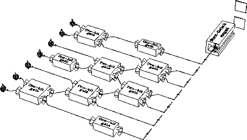
Figure 5: An idealised picture of what a quantum network could look like. Spins enter a network of gates (on the left) and “fly” from one gate to another, where they interact with other qubits (two–bit gates) or are just individually manipulated (one–bit gates). Eventually, at the end of their journey, they are measured by a Stern–Gerlach apparatus.

Deutsch [17] described quantum networks as a possible way to effect complex unitary operations. Quantum networks are composed of elementary logic gates connected together by wires. The only purpose of the wires is to transfer a quantum state from the output of a gate to the input of another one (and eventually to a measurement device). Of course, just as it is the case for quantum gates, the nature of these wires depends on the technological realisations of the qubit. For instance, wires could hypothetically be the trajectories of flying spins: two spins may have their trajectory inflected, enter a zone in which they interact together (a two–bit gate), fly apart again, enter another zone in which they interact with other qubits, etc. (see Fig. 5). The fundamental idea underlying quantum networks is to decompose complex unitary operations acting on several qubits into a sequence of simple one– and two–bit gates. Other paradigms to implement quantum computation involve for instance quantum cellular automata, but so far they have not proved to be tools as valuable as the idea of quantum networks. I will not discuss them here, and the interested reader can refer to the literature on the subject [18].

Deutsch showed that there exists a universal three–bit quantum gate from which any quantum computation, i.e. any unitary operation on any finite number of qubits, can be built by a suitable network consisting only of copies of this gate. This result has been improved upon since then [19] and we now know that almost any non–trivial two–bit gate is universal [20]. Much attention has also been devoted to the efficient construction of more complex quantum gates [21], and to specific networks, such as the one that effects the modular exponentiation required in the first part of the factorisation algorithm [22]. In the following, I will illustrate how the quantum discrete Fourier transform discussed above can be implemented as a network consisting of only one– and two–bit gates.

Consider again the one–bit gate $U_{{\mbox{$\mbox{\scriptsize\sf A}$}}}$ of Sect. 3.2 performing the unitary transformation

$$\begin{array}[]{l}U_{{\mbox{$\mbox{\scriptsize\sf A}$}}}\mbox{$|0\rangle$}=\frac{1}{\sqrt{2}}\;(\mbox{$|0\rangle$}+\mbox{$|1\rangle$})\\ U_{{\mbox{$\mbox{\scriptsize\sf A}$}}}\mbox{$|1\rangle$}=\frac{1}{\sqrt{2}}\;(\mbox{$|0\rangle$}-\mbox{$|1\rangle$}).\end{array}\mbox{\hskip 85.35826pt}\mbox{ \begin{picture}(30.0,0.0)(0.0,15.0)\put(0.0,15.0){$q$} \put(5.0,15.0){\line(1,0){5.0}} \put(20.0,15.0){\line(1,0){5.0}} \put(10.0,10.0){\framebox(10.0,10.0)[]{\sf A}} \end{picture} }$$ (21)

The diagram on the right provides a schematic representation of the gate acting on a qubit $q$. Consider also the two–bit $U_{{\mbox{$\mbox{\scriptsize\sf B}$}}(\phi)}$ gate acting on qubits $q_{1}$ and $q_{2}$ and performing the operation

$$\begin{array}[]{l}U_{{\mbox{$\mbox{\scriptsize\sf B}$}}(\phi)}\mbox{$|00\rangle$}=\mbox{$|00\rangle$}\\ U_{{\mbox{$\mbox{\scriptsize\sf B}$}}(\phi)}\mbox{$|01\rangle$}=\mbox{$|01\rangle$}\\ U_{{\mbox{$\mbox{\scriptsize\sf B}$}}(\phi)}\mbox{$|10\rangle$}=\mbox{$|10\rangle$}\\ U_{{\mbox{$\mbox{\scriptsize\sf B}$}}(\phi)}\mbox{$|11\rangle$}=e^{i\phi}\mbox{$|11\rangle$}.\end{array}\mbox{\hskip 42.67912pt}\mbox{ \begin{picture}(25.0,0.0)(0.0,20.0)\put(-2.0,15.0){$q_{2}$} \put(-2.0,30.0){$q_{1}$} \put(5.0,15.0){\line(1,0){5.0}} \put(20.0,15.0){\line(1,0){5.0}} \put(5.0,30.0){\line(1,0){20.0}} \put(15.0,30.0){\circle*{3.0}} \put(15.0,20.0){\line(0,1){10.0}} \put(10.0,10.0){\framebox(10.0,10.0)[]{$\phi$}} \end{picture} }\equiv\mbox{\hskip 5.69046pt}\mbox{ \begin{picture}(30.0,0.0)(0.0,20.0)\put(-2.0,15.0){$q_{2}$} \put(-2.0,30.0){$q_{1}$} \put(5.0,30.0){\line(1,0){5.0}} \put(20.0,30.0){\line(1,0){5.0}} \put(5.0,15.0){\line(1,0){20.0}} \put(15.0,15.0){\circle*{3.0}} \put(15.0,15.0){\line(0,1){10.0}} \put(10.0,25.0){\framebox(10.0,10.0)[]{$\phi$}} \end{picture} }$$ (22)

The gate $U_{{\mbox{$\mbox{\scriptsize\sf B}$}}(\phi)}$ performs a conditional phase shift, i.e. a multiplication by a phase factor $e^{i\phi}$ only if the two qubits are both in their $|1\rangle$ state. The three other basis states are unaffected.

Figure 6: Network effecting a DFT on a four–bit register, the phases that appear in the operations $U_{{\mbox{$\mbox{\scriptsize\sf B}$}}(\phi_{jk})}$ are related to the “distance” of the qubits upon which $U_{{\mbox{$\mbox{\scriptsize\sf B}$}}}$ acts, namely $\phi_{jk}=\pi/2^{j-k}$. The network should be read from the left to the right: first the gate A is effected on the qubit $a_{3}$, then $B(\phi_{32})$ on $a_{2}$ and $a_{3}$, and so on.

The DFT on a register of any size can be implemented using only these two gates. For example, consider a four–bit register with qubits $a_{0},\ldots a_{3}$. The network in Fig. 6 follows step by step the classical algorithm of a DFT [7], and performs the operation

$$\mbox{$|a\rangle$}\longmapsto\frac{1}{\sqrt{2^{4}}}\sum_{c=0}^{2^{4}-1}\exp(2\pi iac/2^{4})\mbox{$|b\rangle$},$$ (23)

where $|b\rangle$ represents the value $c$ read reversing the order of the bits i.e.

$$b=\sum_{i=0}^{3}2^{i}c_{3-i}\;\;\;\mbox{with $c_{k}$ given by}\;\;\;c=\sum_{k=0}^{3}2^{k}c_{k}.$$ (24)

A trivial extension of the network following the same sequence pattern of gates on $L$ qubits gives the general DFT. In this case the transformation requires $L$ operations $U_{{\mbox{$\mbox{\scriptsize\sf A}$}}}$ and $L(L-1)/2$ operations $U_{{\mbox{$\mbox{\scriptsize\sf B}$}}(\phi)}$, in total $L(L+1)/2$ elementary operations. Thus the quantum DFT can be performed efficiently. Moreover, it can even be simplified [23]: in a general network for DFT, the operations $U_{{\mbox{$\mbox{\scriptsize\sf B}$}}(\phi)}$ that involve distant qubits $a_{j}$ and $a_{k}$, i.e. qubits for which $|j-k|$ is large (and therefore $\phi=\pi/2^{k-j}$ approaches zero), are close to unity. Therefore when performing the quantum DFT on registers of size $L$, one can neglect operations $U_{{\mbox{$\mbox{\scriptsize\sf B}$}}(\phi)}$ on distant qubits (more precisely on qubits $a_{j}$ and $a_{k}$ for which $|j-k|>\log_{2}(L)+2$) and still retrieve the periodicity of coefficients $c_{x}$ with high probability [24].

The network of gates for the quantum DFT enables the efficient implementation of the second part of Shor’s algorithm. The first part requires an efficient quantum evaluation of the function $f_{a,N}(x)=a^{x}\bmod N$. The computation of $f_{a,N}(x)$ is “easy” i.e. the number of elementary operations does not grow faster than a polynomial in the size of the input. The respective network is constructed by combining networks which perform additions and multiplications in a reversible and unitary way [22].

6 Practicalities

It remains an open question which technology will be employed to build the first quantum computers. The conditional quantum dynamics which I alluded to when introducing the operation $U_{{\mbox{$\mbox{\scriptsize\sf B}$}}}$ can be implemented in many different ways, ranging from Ramsey atomic interferometry [25], interacting electrons in quantum dots [26] to ions in ion traps [27] and atoms coupled to high finesse optical resonators [28].

In the following I will present a possible scheme to implement the simple two–bit quantum gate “controlled–NOT” (CNOT) [26]. Its effect on the basis states is

$$\begin{array}[]{l}U_{{\mbox{$\mbox{\scriptsize\sf CNOT}$}}}\mbox{$|00\rangle$}=\mbox{$|00\rangle$}\\ U_{{\mbox{$\mbox{\scriptsize\sf CNOT}$}}}\mbox{$|01\rangle$}=\mbox{$|01\rangle$}\\ U_{{\mbox{$\mbox{\scriptsize\sf CNOT}$}}}\mbox{$|10\rangle$}=\mbox{$|11\rangle$}\\ U_{{\mbox{$\mbox{\scriptsize\sf CNOT}$}}}\mbox{$|11\rangle$}=\mbox{$|10\rangle$}.\end{array}$$ (25)

The gate effects a logical NOT on the second qubit (target bit), if and only if the first qubit (control bit) is in state $1$. Two interacting magnetic dipoles (for instance, the spins we have considered in the previous sections), sufficiently close to each other, can be used to implement this operation. Under carefully chosen conditions [29](complement $\mbox{B}_{\mbox{\scriptsize XI}}$) the total hamiltonian of this system can be written

$$H=H_{1}+H_{2}+H_{\mbox{\scriptsize coupl}}$$ (26)

with

$$\begin{array}[]{l}H_{1}=\hbar\omega_{1}S_{1,z}\\ H_{2}=\hbar\omega_{2}S_{2,z}\\ H_{\mbox{\scriptsize coupl}}=4\hbar\Omega S_{1,z}S_{2,z},\end{array}$$ (27)

where $S_{1,z}$ and $S_{2,z}$ are the $z$ components of the spin operators for spin $1$ and $2$ respectively, so that $S_{1,z}\mbox{$|0,\cdot\rangle$}=-1/2\hbar\mbox{$|0,\cdot\rangle$}$ and $S_{1,z}\mbox{$|1,\cdot\rangle$}=+1/2\hbar\mbox{$|1,\cdot\rangle$}$ (similar relations hold for $S_{2,z}$). $\omega_{i}=\gamma_{i}B_{i}$ depends on the gyromagnetic ratio $\gamma_{i}$ of spin $i$ and of the magnetic field $B_{i}$ (along the $z$ axis) experienced by spin $i$. We will suppose that either the magnetic fields or the gyromagnetic ratios are different for each qubit so that $\omega_{1}\neq\omega_{2}$. Finally $\Omega$ is a coupling factor that depends, among others, on the distance between the two spins and their relative orientation. The form of the above hamiltonian is valid under the assumption that the coupling $\Omega$ is small enough to be regarded as a perturbation.

Without coupling ($\Omega=0$, for instance when both spins are sufficiently far apart), each spin can be selectively flipped by a resonant electromagnetic field of appropriate duration and intensity: shining a pulse at frequency $\omega_{1}$ on both spins will affect only spin $1$, switching it from state $|0,\cdot\rangle$ (spin down) to $|1,\cdot\rangle$ (spin up), and vice versa. Similarly, a pulse of frequency $\omega_{2}$ will only affect spin $2$.

When both spins are close enough to interact ($\Omega>0$), the situation is more complicated and one needs to find the eigenstates of the hamiltonian $H$. Fortunately, $H$ remains diagonal in the basis $\{\mbox{$|00\rangle$},\mbox{$|01\rangle$},\mbox{$|10\rangle$},\mbox{$|11\rangle$}\}$ and the energies of the eigenstates are shifted by $\pm\hbar\Omega$, depending on the state (cf. Fig. 7a). By carefully selecting a resonant frequency, it is now possible to induce selective switching of one spin depending on the state of the other. Fig. 7 illustrates how a pulse of frequency $\omega_{2}+\Omega$ induces a switching betweeen states $|10\rangle$ and $|11\rangle$ only, leaving states $|00\rangle$ and $|01\rangle$ unaffected, implementing thus the CNOT operation.

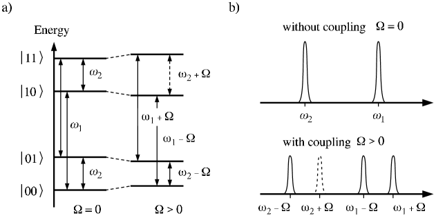
Figure 7: (a) Eigenenergies of the basis state of two spins without and with coupling. (b) Resonant frequencies of the two spins without and with coupling. When there is no coupling, the two frequencies are made different for instance, by putting each spin in a magnetic field of slightly different intensity. With coupling, each resonant frequency is split into two frequencies; if the splitting is sufficient, it is possible to select specific transitions. The dotted transition corresponds to the CNOT operation, in which only states $|10\rangle$ and $|11\rangle$ are affected.

Obviously the above description is rather simplistic and does not include any unwelcome effects; however, the form of the hamiltonian $H$ and of the coupling $H_{\mbox{\scriptsize coupl}}$ appears in many radically different contexts (excitons or electrons in quantum dots [26], interacting Cooper pairs in superconducting islands [30]), and is general enough to make this setup worth mentioning.

6.1 Coupling with the environment: the decoherence problem.

In order to perform a successful quantum computation, one has to maintain a coherent unitary evolution until the completion of the computation. Technically it is not possible to ensure that a quantum register is completely isolated from the environment. This remnant coupling induces decay and decoherence processes, both of which drastically reduce the performance of a quantum computer, even when the coupling is very weak. Decay is a process by which a quantum system dissipates energy in the environment. For a spin, it is for instance a transition from $\mbox{$|1\rangle$}\longrightarrow\mbox{$|0\rangle$}$, accompanied by the emission of a photon of appropriate wavelength. Decoherence is a subtler phenomenon that involves no exchange of energy with the environment [31]. Its effect is to scramble the relative phase of the various parts of a quantum superposition. Decoherence occurs in most cases on a much faster timescale than decay, and therefore, I will focus on this kind of processes.

Decoherence can be more easily understood if we formalise it in the language of density operators, rather than in the more familiar Dirac notation. When a quantum system is in a pure state, it can be equivalently described by a ket $|\psi\rangle$ or by a density operator $\rho=\mbox{$|\psi\rangle$}\mbox{$\langle\psi|$}$. The characteristic effect of decoherence is to destroy the off–diagonal elements of the density operator; the system evolves into a “mixed state” [29] for which the ket notation is no longer suitable. To see how this can affect quantum computers, let me first consider the very simple situation in which a qubit initially in the state $|0\rangle$ undergoes successively and without decoherence two operations $U_{{\mbox{$\mbox{\scriptsize\sf A}$}}}$ (as introduced in Sect. 3.2):

$$\mbox{$|\psi_{in}\rangle$}=\mbox{$|0\rangle$}\stackrel{{\scriptstyle U_{{\mbox{$\mbox{\tiny\sf A}$}}}}}{{\longrightarrow}}\frac{1}{\sqrt{2}}(\mbox{$|0\rangle$}+\mbox{$|1\rangle$})\stackrel{{\scriptstyle U_{{\mbox{$\mbox{\tiny\sf A}$}}}}}{{\longrightarrow}}\mbox{$|0\rangle$}=\mbox{$|\psi_{fin}\rangle$}.$$ (28)

In a density matrix formulation, this sequence can be written (in the basis ${\cal B}=\{\mbox{$|0\rangle$},\mbox{$|1\rangle$}\}$)

$$\rho_{in}=\mbox{$\left(\begin{array}[]{cc}1&0\\ 0&0\end{array}\right)$}\stackrel{{\scriptstyle U_{{\mbox{$\mbox{\tiny\sf A}$}}}}}{{\longrightarrow}}\frac{1}{2}\mbox{$\left(\begin{array}[]{cc}1&1\\ 1&1\end{array}\right)$}\stackrel{{\scriptstyle U_{{\mbox{$\mbox{\tiny\sf A}$}}}}}{{\longrightarrow}}\mbox{$\left(\begin{array}[]{cc}1&0\\ 0&0\end{array}\right)$}=\rho_{fin}.$$ (29)

A measurement of the final state would yield $0$ with probability one. Let me suppose now that decoherence occurs in between the two operations $U_{{\mbox{$\mbox{\scriptsize\sf A}$}}}$ and wipes out completely the off–diagonal elements (this is of course an oversimplification, and one should rather picture decoherence as a continuous process that progressively eliminates the off–diagonal elements). In this case, the sequence of operations reads

$$\rho_{in}=\mbox{$\left(\begin{array}[]{cc}1&0\\ 0&0\end{array}\right)$}\stackrel{{\scriptstyle U_{{\mbox{$\mbox{\tiny\sf A}$}}}}}{{\longrightarrow}}\frac{1}{2}\mbox{$\left(\begin{array}[]{cc}1&1\\ 1&1\end{array}\right)$}\stackrel{{\scriptstyle\mbox{ \tiny\sf DECO.}}}{{-\!\!\!-\!\!\!-\!\!\!\!\longrightarrow}}\frac{1}{2}\mbox{$\left(\begin{array}[]{cc}1&0\\ 0&1\end{array}\right)$}\stackrel{{\scriptstyle U_{{\mbox{$\mbox{\tiny\sf A}$}}}}}{{\longrightarrow}}\frac{1}{2}\mbox{$\left(\begin{array}[]{cc}1&0\\ 0&1\end{array}\right)$}=\tilde{\rho}_{fin},$$ (30)

and $\tilde{\rho}_{fin}$ no longer represents a qubit in the state $|0\rangle$, but rather a statistical mixture of the states $|0\rangle$ and $|1\rangle$. Performing a measurement on the qubit would now return either $0$ or $1$ with equal probability; thus decoherence affects the probability distribution of the possible outcomes of a computation.

The onset of decoherence is actually more complex, and to a large extent depends on the physical situation. In a typical case, for a quantum computer of $S$ qubits which interacts with the environment in a thermal equilibrium, the off–diagonal elements of the density matrix decay exponentially fast at a rate $\gamma S$ [32]

$$\rho_{ij}(t)\sim\rho_{ij}(0)e^{-\gamma St}$$ (31)

where $\gamma=1/\tau_{dec}$ is a constant that describes the coupling of a single qubit with the environment: the stronger the coupling, the higher $\gamma$ and the smaller the decoherence time $\tau_{dec}$.

For an efficient computation, we have seen that both $S$ and the total computation time $t_{tot}$ required to complete the algorithm should not grow faster than a polynomial, so that one can write

$$S\sim L^{\alpha}\qquad t_{tot}\sim L^{\beta}t_{elem},$$ (32)

where $t_{elem}$ is the characteristic time needed to perform a single elementary computational step of the algorithm. From this, it is then possible to show that the probability $\cal P$ of measuring the right answer at the end of the quantum computation decreases exponentially with $S$ and $t_{tot}$, and hence with $L^{\alpha+\beta}$:

$${\cal P}\simeq e^{-\gamma St_{tot}}=e^{-\gamma t_{elem}L^{\alpha+\beta}}.$$ (33)

This can be illustrated in a very simple situation. Consider performing a DFT on a register of $L$ qubits that encodes a superposition of period $r=4$. Without decoherence, we expect, according to Eq. (20), to measure with equal probability either $|0\rangle$, $|2^{L-2}\rangle$, $|2\cdot 2^{L-2}\rangle$ or $|3\cdot 2^{L-2}\rangle$. The measurement outcome will be affected by decoherence and Fig. 8 illustrates how the diagonal elements of the density matrix of the state (i.e. the probability outcomes of a measurement) behave. The calculation is repeated for different $L$ with the same amount of decoherence (given by a fixed $\gamma$).

Figure 8: Numerical simulations that mimic the effect of decoherence on the result of a DFT. The initial state (not shown) is a periodic state with $r=4$ on a register of varying size (see Fig. 3 for the case $L=8$). Without decoherence, the resulting state should have only $4$ components (Fig. 3b). The coupling with the environment induces errors (a-d), and reduces the probability of measuring the right answer. For a fixed $\gamma$ and increasing $L$, the probability of getting the right peak decreases in a characteristic exponential way (central plot). The four plots a), b), c) and d) show the diagonal elements of the density matrix of the output. The intensity of the four principal peaks decreases as $L$ increases, and the probability of measuring a correct result decreases in an exponential fashion (central plot). Note that the scales on the vertical axis are adjusted for graphs c) and d).

To obtain at least one successful computation, one needs to run the computer on average $1/{\cal P}=e^{\gamma t_{elem}L^{\alpha+\beta}}$ times. Thus the problem becomes exponentially difficult as soon as some decoherence is present. From the complexity point of view, the magnitude of $\gamma$ has no relevance: as soon as there is some coupling with the environment and $\gamma$ is non–zero, any computation becomes inefficient. It is however quite clear that for small $\gamma$ (long decoherence time $\tau_{dec}=1/\gamma$), it is possible to effect some quantum operations before decoherence takes its toll. Technological progress in isolating quantum computers from the environment and reducing decoherence will increase the largest number that can be factored by such computers. The requirement for a coherent computation to be completed within the decoherence time can be written as

$$t_{tot}<\tau_{dec}/S=\tau_{dec}/L^{\alpha}.$$ (34)

The right–hand side is the characteristic decoherence time of $L^{\alpha}$ qubits. From the above it follows that

$$L<\left(\frac{\tau_{dec}}{t_{elem}}\right)^{1/(\alpha+\beta)}.$$ (35)

With the best implementation of the factorisation algorithm $\alpha=1$ and $\beta=3$ [22], hence the size of the largest number that can be factored is bounded by $L<(\tau_{dec}/t_{elem})^{1/4}$. This is an optimistic estimate in which only decoherence is taken into account. A careful analysis shows that this bound is dramatically reduced when decay phenomena (such as spontaneous emission) are also included [33].

The ratio ${\cal M}=\tau_{dec}/t_{elem}$ is a useful figure of merit for comparing different technologies. It tells us, very approximatively, how many elementary operations can in principle be performed on a single qubit before it decoheres. Table 2 summarises these values for some of the technologies that could be used to implement basic quantum computations. Some of these have already been used to implement fundamental two–bit gates (such as the CNOT operation) [34]. It is however still too early to say if the present experimental setups can be scaled up easily and if these technologies can be used to implement computations on many qubits.

Technology $t_{elem}$ $\tau_{dec}$ $\cal M$ Mössbauer nucleus $10^{-19}$ $10^{-10}$ $10^{9}$ Electrons GaAs^⋆ $10^{-13}$ $10^{-10}$ $10^{3}$ Electrons Au $10^{-14}$ $10^{-8}$ $10^{6}$ Trapped ions^⋆ $10^{-14}$ $10^{-1}$ $10^{13}$ Optical cavities $10^{-14}$ $10^{-5}$ $10^{9}$ Electron spin $10^{-7}$ $10^{-3}$ $10^{4}$ Electron quantum dot^⋆ $10^{-6}$ $10^{-3}$ $10^{3}$ Nuclear spin $10^{-3}$ $10^{4}$ $10^{7}$ Superconductor islands^⋆ $10^{-9}$ $10^{-3}$ $10^{6}$

Table 2: Figure of merit $\cal M$ for different technologies. The table gives respectively the characteristic decoherence time $\tau_{dec}$, the (minimum) time to complete an elementary operation $t_{elem}$ (defined as $t_{elem}\simeq\hbar/\Delta E$, where $\Delta E$ is the energy splitting between the two states $|0\rangle$ and $|1\rangle$ of the qubit) and the number of operations $\cal M$ that could in principle be effected on a qubit before decoherence takes over. Asterisks indicate that the numbers given are to a large extent speculative. The values are taken from [35].

7 Conclusion

As was the case in quantum cryptography a few years ago, the field of quantum computation is rapidly growing and has already begun to move from a theoretical to an experimental phase. Whether a full quantum computer will ever be built remains an open question. The technological challenge is immense and many problems must be overcome first. A quantum computation requires coherent quantum evolution on a macroscopic scale. Not only that, it also needs to be actively controlled. At present, we know of very few macroscopic quantum states that involve many particles, or subsystems (e.g. electrons in a superconductor, ⁴He atoms in a superfluid, or the recently observed Bose–Einstein condensates of Rb, Na or Li atoms); in each case, the state is globally quantum and the particles are not controlled on an individual basis. We may argue that each of these quantum systems performs a quantum computation in its own, but it may not be a computation we are interested in and moreover, we have no real control over it.

The fragility of these macroscopic quantum systems tells us much about the effect of decoherence. As explained in the last section, decoherence ultimately cuts out any “exponential” speed–up that we may gain from using quantum computers and quantum algorithms, simply because to overcome it, the best technique so far is to run the same computation over and over again an exponential number of times (until we get a correct answer). Fortunately, this is not the end of the story. Classical computers suffer from similar problems, and yet, one tends to agree that classical computers are (in general!) reliable. This is because in the classical situation we have efficient ways to fight errors. For existing computers, error–correcting codes have been designed that are exponentially effective and that can handle and control possible errors. Unfortunately, these techniques cannot be directly translated to tame decoherence in quantum computers. They are based on redundancy (i.e. several bits encoding one bit of information), and more importantly, on a periodic monitoring of the state of the computer. Periodic monitoring means, grosso modo, measuring the state of the computer, diagnosing an eventual error (and eventually correcting it); but as we have seen, the mere act of performing a measurement on a quantum computer will alter its state. This obliges us to rethink the problem of error–correction in quantum terms. First promising steps in this direction have already been made [36].

From a fundamental point of view, it is irrelevant whether or not a “quantum personal computer” will materialise in the next decade. More important is the insight we will gain in their study. Quantum computation already tells us a lot about the deep connections between physics, computation and more generally information theory. No doubt there is much more to learn.

Acknowledgements

I would like to thank P.L. Knight, M. Abouzeid, T. Brun, A. Ekert, C. Macchiavello, A. Sanpera, and K.–A. Suominen for useful and critical comments during the preparation of this manuscript. I am supported by the Berrow fund at Lincoln College, Oxford, which I acknowledge gratefully.

Appendix A Discrete Fourier Transform

Let us consider the simplified situation where the period $r$ divides $2^{L}$ exactly. A register in a periodic state is given for instance by Eq. (16), which we rewrite

$$\mbox{$|\phi_{in}\rangle$}=\sqrt{\frac{r}{2^{L}}}\;\sum_{j=0}^{G}\mbox{$|jr+l\rangle$}=\sum_{x=0}^{2^{L}-1}c_{x}\mbox{$|x\rangle$}$$ (36)

with $G=2^{L}/r$. Performing a DFT on $|\phi_{in}\rangle$ gives

$$\mbox{$|\phi_{out}\rangle$}=\sum_{y}c_{y}\mbox{$|y\rangle$},$$ (37)

where the amplitude of $c_{y}$ is

$$c_{y}=\frac{\sqrt{r}}{2^{L}}\sum_{j=0}^{G}\exp\left(\frac{2\pi i(jr+l)y}{2^{L}}\right)=\frac{\sqrt{r}}{2^{L}}\exp\left(2\pi i\frac{ly}{2^{L}}\right)\left[\sum_{j=0}^{G}\exp\left(2\pi i\frac{jry}{2^{L}}\right)\right].$$ (38)

The term in the square bracket on the r.h.s. is zero unless $y$ is a multiple of $2^{L}/r$,

$$c_{y}=\left\{\begin{array}[]{ll}\exp(2\pi ily/2^{L})/\sqrt{r}&\mbox{if $y$ is a multiple of $2^{L}/r$: $y=k2^{L}/r$ }\\ 0&\mbox{otherwise}\end{array}\right.$$ (39)

Therefore, in the particular case when $r$ divides $2^{L}$ exactly, $|\phi_{out}\rangle$ can be written

$$\mbox{$|\phi_{out}\rangle$}=\frac{1}{\sqrt{r}}\sum_{k=0}^{r-1}\exp(2\pi ilk/r)\;\mbox{$|k2^{L}/r\rangle$}.$$ (40)

A more elaborate analysis is actually required when $r$ is not a multiple of $2^{L}$. In this case, after effecting the DFT, the coefficients $c_{y}$ are peaked on the closest integers to the multiples of $2^{L}/r$ (cf. Fig. 9). These peaks have a spread that decreases exponentially with $L$ (hence the reason to choose in the factorisation algorithm the size of the first register to be 2L). A careful analysis of this case can be found in [16].

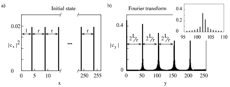
Figure 9: Same as Fig. 3, but in this case $r=5$ does not divide exactly $2^{L}=256$. This results in a broadening of the peaks of the output state $\sum_{y}c_{y}\mbox{$|y\rangle$}$. Nevertheless, it can be shown that, when effecting a measurement on this state, the closest integers from multiples of $2^{L}/r$ are the most likely outcomes. This is illustrated in the inset: $102$ (local maximum), is the closest integer of $2\times 2^{8}/5=102.4$. (Normally one plots $|c_{y}|^{2}$, i.e., the actual probabilities, but here $|c(y)|$ is plotted to emphasise the spread of the peaks.)

References

- [1] R. Landauer, IBM J. Res. Dev. 5, 183 (1961); C.H. Bennett, IBM J. Res. Dev. 17, 525 (1973); C.H. Bennett, Int. J. Theor. Phys. 21, 905 (1982); C.H. Bennett, SIAM J. Comput. 18(4), 766 (1989).
- [2] D. Deutsch, D., Proc. R. Soc. London A 400, 97 (1985).
- [3] P.W. Shor, in Proceedings of the 35th Annual Symposium on the Foundations of Computer Science, edited by S. Goldwasser (IEEE Computer Society Press, Los Alamitos, CA), p. 124 (1994).
- [4] R. Rivest, A. Shamir, L. Adleman, On Digital Signatures and Public–Key Cryptosystems, MIT Laboratory for Computer Science, Technical Report, MIT/LCS/TR-212 (January 1979).
- [5] D. Welsh, Codes and cryptography, Clarendon Press, Oxford, (1988). H. S. Wilf, Algorithms and complexity, Prentice-Hall, Englewood Cliffs / Prentice-Hall International, London, (1986).
- [6] A.K. Lenstra, H.W. Lenstra Jr., M.S. Manasse, and J.M. Pollard, in Proc. 22nd ACM Symposium on the Theory of Computing, p.564 (1990).
- [7] D.E. Knuth, The Art of Computer Programming, Volume 2: Seminumerical Algorithms (Addison-Wesley, 1981).
- [8] B. Schumacher, Phys. Rev. A 51, 2738 (1995).
- [9] A.S. Holevo, Problemy Peredachi Informatsii, 9, 3 (1979) (this journal is translated by IEEE under the title Problems of Information Transfer); E.B. Davies, IEEE Trans. Inform. Theory, IT 24, 596 (1978); C.A. Fuchs and C.M. Caves, Phys. Rev. Lett. 73, 3047 (1994).
- [10] S. Wiesner, Sigact News 15(1), 78 (1983); C.H. Bennett and G. Brassard in Proceedings of the IEEE International Conference on Computers, Systems, and Signal Processing, Bangalore, India pp175, (IEEE, New York, 1984); A. Ekert, Phys. Rev. Lett. 71, 4287 (1993). For a review of the field, see also R.J. Hughes, D.M. Alde, P. Dyer, G.G. Luther, G.L. Morgan and M. Schauer, Contemporary Physics 36(3), 149 (1995); and also S.J.D. Phoenix and P.D. Townsend, Contemporary Physics 36(3), 165 (1995).
- [11] C.H. Bennett, G. Brassard, C. Crépeau, R. Jozsa, A. Peres, and W.K. Wootters, Phys. Rev. Lett. 70, 1895 (1993).
- [12] C.H. Bennett and S. Wiesner, Phys. Rev. Lett. 69, 2881 (1992).
- [13] A. Peres, Quantum Theory: Concepts and Methods (Kluwer, 1993).
- [14] G.H. Hardy and E.M. Wright: An Introduction to the Theory of Numbers (4th edition, Oxford University Press, 1965).
- [15] G.L. Miller, Journal of Computer Science 13, 300 (1976);
- [16] A. Ekert and R. Jozsa, Rev. Mod. Phys. to appear 1996.
- [17] D. Deutsch, Proc. R. Soc. London A 425, 73 (1989).
- [18] N. Margolus, in Complexity, Entropy, and the Physics of Information, edited by W. Zurek (Addison-Wesley) 1990; M. Biafore, MIT Ph.D. Thesis (1993).
- [19] A. Barenco, Proc. R. Soc. London A 449, 679 (1995); D.P. DiVincenzo, Phys. Rev. A 50, 1015 (1995); T. Sleator and H. Weinfurter, Phys. Rev. Lett. 74, 4087 (1995).
- [20] D. Deutsch, A. Barenco and A. Ekert, Proc. R. Soc. London A 449, 669 (1995); S. Lloyd, Phys. Rev. Lett. 75, 346 (1995).
- [21] A. Barenco, C.H. Bennett, R. Cleve, D.P. DiVincenzo, N. Margolus, P. Shor, T. Sleator, J. Smolin and H. Weinfurter, Phys. Rev. A 52, 3457 (1995); J.A. Smolin and D.P. DiVincenzo, Five Two-Bit Quantum Gates are Sufficient to Implement the Quantum Fredkin Gate, preprint 1995.
- [22] V. Vedral, A. Barenco and A. Ekert, Quantum Networks for Elementary Operations, submitted to Phys. Rev. A.
- [23] D. Coppersmith, IBM Research Report No. RC19642 (1994). D. Deutsch, unpublished.
- [24] A. Barenco, A. Ekert, P. Törmä and K.–A. Suominen, On quantum implementation of the discrete Fourier transform and related algorithms, submitted to Phys. Rev. A.
- [25] M. Brune, P. Nussenzveig, F. Schmidt-Kaler, F. Bernardot, A. Maali, J.M. Raimond and S. Haroche, Phys. Rev. Lett. 72, 3339 (1994).
- [26] A. Barenco, D. Deutsch, A. Ekert and R. Jozsa, Phys. Rev. Lett. 74, 4083 (1995).
- [27] J.I. Cirac and P. Zoller, Phys. Rev. Lett 74, 4091 (1995).
- [28] Q.A. Turchette, C.J. Hood, W. Lange, H. Mabuchi and H.J. Kimble, Measurement of conditional phsae shifts for quantum logic, Caltech preprint.
- [29] See for example C. Cohen-Tannoudji, B. Diu, F. Laloë, Quantum Mechanics (Hermann and John Wiley & Sons, 1977).
- [30] M. Devoret, private communication.
- [31] See for instance W.H. Zurek, Physics Today, 44(10), 36 (1991).
- [32] W.G. Unruh, Phys. Rev. A 51, 992 (1995); G.M. Palma, K.–A. Suominen and A. Ekert, 1995, Decoherence in quantum registers, to be published in Proc. R. Soc. London A. This phenomenon has been known for a while in other contexts, see for instance S.M. Barnett and P.L. Knight, Phys. Rev. A 33, 2444 (1986) for an example in quantum optics.
- [33] M. Plenio and P.L. Knight, Realistic Lower Bounds for the Factorisation Time of Large Numbers on a Quantum Computer, submitted to Phys. Rev. A.
- [34] C. Monroe et al., Phys. Rev. Lett. 75, 4714 (1995).
- [35] D. DiVincenzo, Phys. Rev. A, 50, 1015 (1995).
- [36] A. Steane, Multiple Particle Interference and Quantum Error Correction, submitted to Proc. R. Soc. London A; A.R. Calderbank and P.W. Shor, preprint.; see also P.W. Shor, Phys. Rev. A 52, R2493 (1995).