The AC Stark, Stern-Gerlach,
and Quantum Zeno Effects
in Interferometric Qubit Readout

Abstract

This article describes the AC Stark, Stern-Gerlach, and Quantum Zeno effects as they are manifested during continuous interferometric measurement of a two-state quantum system (qubit). A simple yet realistic model of the interferometric measurement process is presented, and solved to all orders of perturbation theory in the absence of thermal noise. The statistical properties of the interferometric Stern-Gerlach effect are described in terms of a Fokker-Plank equation, and a closed-form expression for the Green’s function of this equation is obtained. Thermal noise is added in the form of a externally-applied Langevin force, and the combined effects of thermal noise and measurement are considered. Optical Bloch equations are obtained which describe the AC Stark and Quantum Zeno effects. Spontaneous qubit transitions are shown to be observationally equivalent to transitions induced by external Langevin forces. The effects of delayed choice are discussed. The results are relevant to the design of qubit readout systems in quantum computing, and to single-spin detection in magnetic resonance force microscopy.

The subject of this article is the statistical behavior of interferometric methods for observing two-state quantum systems (henceforth called qubits). Our analysis is motivated by engineering and applied physics considerations — we wish to determine such things as measurement times, error rates, and whether noise-induced transitions can be suppressed by interferometric measurement (the Quantum Zeno effect).

We shall consider interferometric measurements that are ideal in the following respects: (1) photons are detected with 100% efficiency, (2) the qubit-photon interaction does not alter the helicity or wavelength of the photons, nor does it scatter them out of the interferometer, and (3) qubit basis states exist such that the qubit-photon interaction does not induce transitions between the basis states. With these restrictions, the most general scattering amplitude between an initial qubit state ${\big{|}}{\mathrm{initial}}{\big{>}}$ with an incoming photon state and a final qubit state ${\big{|}}{\mathrm{final}}{\big{>}}$ with an outgoing photon state is

$${\big{|}}{\mathrm{final}}{\big{>}}\otimes{\big{|}}{\mathrm{outgoing\ photon}}{\big{>}}=U{\big{|}}{\mathrm{initial}}{\big{>}}\otimes{\big{|}}{\mathrm{incoming\ photon}}{\big{>}}\ ,$$ (1)

where $U$ is a unitary matrix acting on the two-dimensional qubit states. We remark that a photon-state phase shift — which according to our assumptions is the only permissible alteration of the photon state — can always be absorbed into $U$, so that $U$ encompasses a completely general description of interferometric interactions subject to idealizing assumptions 1–3 above. By an appropriate choice of basis, $U$ can always be written as

$$U=\exp\left[i(\phi I+\theta\sigma_{z})\right]\,,$$ (2)

where $\sigma_{z}$ is the usual $2\times 2$ Pauli spin matrix normalized such that $\sigma_{z}^{2}=I$, and $I$ is the identity matrix. We shall see that the overall phase shift $\phi$ can be set to zero without loss of generality.

It is evident that when the initial qubit state is an eigenstate of $\sigma_{z}$, the sole effect of the qubit-photon interaction is a state-dependent phase shift of the outgoing photon by $\pm\theta$, as per idealizing assumption (3) above. We shall be particularly interested in measurement processes in which $\theta$ is a small number, $\theta\sim 10^{-6}$ or less, such that $U$ minimally perturbs the qubit state, as is consistent with real-world interferometry.

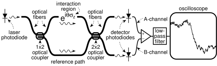
Figure 1: Interferometer for measuring a two-state system.

We next describe the detection of the phase shift by an optical interferometer of conventional design. For concreteness we shall discuss a device fabricated of single-mode optical fiber components, as illustrated in Fig. 1. Emitted photons pass through a beam splitter in the form of a $1\times 2$ single-mode optical coupler. Photons can take either of two paths: an upper signal path which interacts with the qubit system via Eq. 1, and a lower reference path which leads straight to the $2\times 2$ optical coupler which serves as the beam combiner. The output fibers are connected to conventional photodiodes, designated as the A-channel and B-channel in Fig. 1.

As is usual in optical interferometry [5], we stipulate that the reference path length has been adjusted such that the device is fringe-centered, i.e., for a classical phase shift $\theta$ within the interaction region, the probability of photon detection on the A-channel is $(1+\sin(\theta))/2$, while on the B-channel it is $(1-\sin(\theta))/2$. The effect of the residual phase $\phi$ in Eq. 2 is thereby adjusted to zero.

For experiments conducted with a qubit in the interaction region, the data record consists of a sequence of A-channel and B-channel detected photons: $\{a,b,a,b,\ldots,b,a,b\}$. Given a starting qubit state ${\big{|}}{\mathrm{initial}}{\big{>}}$ and a measured data sequence $\{a,b,a,b,\ldots,b,a,b\}$, we ask: what is the qubit state ${\big{|}}{\mathrm{final}}{\big{>}}$ at the end of the experiment? For the interferometer described above it is readily shown from Eqs. 1 and 2 that the transition matrix is

$${\big{|}}{\mathrm{final}}{\big{>}}=ABAB\cdots BAB\ {\big{|}}{\mathrm{initial}}{\big{>}}\,,$$ (3)

where the $A$ and $B$ matrices are

$$A = {\frac{1}{2}}\ \left((\cos(\theta)+i)I+\sin(\theta)\sigma_{z}\right)\,,$$ (4)

$$B = {\frac{1}{2}}\ \left((\cos(\theta)-i)I+\sin(\theta)\sigma_{z}\right)\,.$$ (5)

The qubit state ${\big{|}}{\mathrm{final}}{\big{>}}$ as defined by Eq. 3 is unnormalized; the probability of measuring a specified data sequence $P(\{a,b,a,b,\ldots,b,a,b\})$ is therefore

$$P(\{a,b,a,b,\ldots,b,a,b\}) = {\big{<}}{\mathrm{final}}|{\mathrm{final}}{\big{>}}$$ (6)

$$= \left|\,ABAB\cdots BAB{\big{|}}{\mathrm{initial}}{\big{>}}\,\right|^{2}\,.$$

The $A$ and $B$ matrices satisfy $A^{\dagger}A+B^{\dagger}B=I$; this ensures that the probability of each possible data sequence, summed over all possible data sequences, is unity.

Equations 1–6 are the starting point of our analysis. It should be noted that this system of equations can be regarded as a specific example of a well-accepted general formalism in quantum measurement theory — extensively discussed by, e.g., Barchielli and Belavkin [1] — in which the final state associated with each possible data record is constructed a posteriori.

Because $[A,B]=0$ — later on we will discuss experiments involving control feedback which do not satisfy this condition — $P$ can be written in a particularly simple form:

$$P(\{a,b,a,b,\ldots,b,a,b\}) = {\big{<}}{\mathrm{initial}}|(A^{\dagger}A)^{n_{a}}\,(B^{\dagger}B)^{n_{b}}|{\mathrm{initial}}{\big{>}}$$ (7)

$$= P(n_{a},n_{b})\,.$$

Here $n_{a}$ and $n_{b}$ are the numbers of photons measured on the A-channel and B-channel respectively.

It is physically significant that $P$ depends only on $n_{a}$ and $n_{b}$, and not on the order in which the A-channel and B-channel photons are detected. In consequence, any experimental record can be randomly permuted to obtain an equally probable record; thus the early portions of the data record are statistically indistinguishable from later portions, and it is impossible, even in principle, to identify any moment during the measurement process at which the qubit wave function collapses, even from a retrospective review of an entire experimental record.

It is convenient to parametrize $P(n_{a},n_{b})$ in terms of a single variable $q\equiv(n_{a}-n_{b})/((n_{a}+n_{b})\theta)$. Physically, $q$ is the differential photodiode charge, with gain adjusted (with foresight) such that $q=\pm 1$ is the expected value in the presence of the Stern-Gerlach effect. To characterize the initial qubit states, we define a qubit polarization variable $z_{0}$:

$$z_{0}\equiv{\big{<}}{\mathrm{initial}}|\sigma_{z}|{\mathrm{initial}}{\big{>}}\,.$$ (8)

Substituting the explicit forms of $A$ and $B$ in Eq. 7, and changing variables, we obtain the probability density $P(q|z_{0},t)$ for measuring $q$ after time $t$:

$$P(q|z_{0},t)=\left[\frac{tr\theta^{2}}{2\pi}\right]^{1/2}\left[\frac{(1+z_{0})}{2}\,e^{-tr\theta^{2}(q-1)^{2}/2}+\frac{(1-z_{0})}{2}\,e^{-tr\theta^{2}(q+1)^{2}/2}\right]\,.$$ (9)

Here $r$ is the photon flux in photons/second, and terms of order $\theta^{3}$ and higher have been dropped. These terms are negligible in practice, since $\theta\sim 10^{-6}$ or smaller is typical of optical interferometry.

We note that $P(q|z_{0},t)$ can be written in a form in which $z_{0}$ enters only as an overall statistical weight:

$$P(q|z_{0},t)=\frac{(1+z_{0})}{2}P(q|\,1,t)+\frac{(1-z_{0})}{2}P(q|-\!\!1,t)\,.$$ (10)

This result implies that it is impossible, even in principle, to experimentally distinguish between (1) a succession of experiments, each having identical starting polarization $z_{0}=\beta$, and (2) a succession of experiments, each having randomly assigned starting polarizations of $z_{0}=\pm 1$, such that $z_{0}=1$ with probability $(1+\beta)/2$ and $z_{0}=-1$ with probability $(1-\beta)/2$.

In summary, the nature of interferometric qubit measurements is such that, for sufficiently long measurement times, the measured photodiode charge $q$ is always either $+1$ or $-1$ (Eq. 9) — this is the Stern-Gerlach effect. However, even retrospective review of the entire experimental record cannot identify any moment at which the qubit wave function collapses (Eq. 7). Furthermore, interferometric measurements cannot distinguish an ensemble of identical qubit states from a randomly mixed ensemble of differing states with the same average value of $z_{0}$ (Eq. 10). These findings collectively imply that interferometric measurement obeys the general quantum-mechanical principle that at most one bit of information can be obtained from measurement of a two-state system [11].

Having characterized the statistical evolution of the macroscopic photodiode charge $q$ in complete detail, we now describe the evolution of the microscopic qubit polarization variable $z$:

$$z\equiv{\big{<}}{\mathrm{final}}|\sigma_{z}|{\mathrm{final}}{\big{>}}\,,$$ (11)

where we specify that ${\big{|}}{\mathrm{final}}{\big{>}}$ (obtained from Eq. 3) is to be normalized prior to computing $z$. From the expressions for $A$ and $B$ (Eq. 5) it can be shown that that $z$ evolves according to $dz=(1-z^{2})\theta\,(dn_{a}-dn_{b})$. Then from $P(q|z_{0},t)$ (Eq. 9) we can readily infer a closed-form expression for the distribution $P(z|z_{0},t)$ which describes the statistical evolution of $z$:

$$P(z|z_{0},t) = \frac{1}{1-z^{2}}\left(\frac{1-z_{0}^{2}}{8\pi tr\theta^{2}}\right)^{1/2}\left(\left(\frac{1+z}{1-z}\right)^{1/2}+\left(\frac{1-z}{1+z}\right)^{1/2}\right)$$ (12)

$$\times\exp\left[\frac{-1}{8tr\theta^{2}}\left(\ln\left(\frac{1+z}{1-z}\right)-\left(\frac{1+z_{0}}{1-z_{0}}\right)\right)^{2}-\frac{tr\theta^{2}}{2}\right].$$

By direct substitution we verify that this unwieldy expression is the Green’s function of a simple and physically illuminating Fokker-Planck equation:

$$\frac{\partial P}{\partial t}=r\theta^{2}\,\frac{\partial}{\partial z}\left(D(z)\frac{\partial P}{\partial z}-V(z)P\right)\,.$$ (13)

Here $D(z)\equiv(1-z^{2})^{2}/2$ plays the role of a diffusion coefficient, and $V(z)\equiv 2z(1-z^{2})=-dD(z)/dz$ is a drift velocity.

This equation has a ready physical interpretation. From Eqs. 3 and 11 it can be shown that the microscopic qubit polarization $z(t)$ evolves as a Markovian random process. Qubits with $z\sim 0$ experience maximal diffusion $D(z)$: they rapidly diffuse away from $z\sim 0$. Once diffusion has begun, it is hastened by the drift velocity $V(z)$, which acts to push qubits away from $z\sim 0$ and toward $|z|\sim 1$. As qubit states approach extremal values of $|z|\sim 1$, both $D(z)$ and $V(z)$ go to zero. In the absence of thermal noise or spontaneous transitions — we consider these phenomena later on — a qubit state never evolves away from the limiting values $z=\pm 1$, as shown by the asymptotic form of the Green’s function:

$$P(z|z_{0},t)\stackrel{{\scriptstyle t\rightarrow\infty}}{{=}}\frac{(1+z_{0})}{2}\delta(z-1)+\frac{(1-z_{0})}{2}\delta(z+1)\,.$$ (14)

This is the Stern-Gerlach effect as manifest in the evolution of the quantum variable $z$; it is the microscopic analog of Eq. 10.

Quantum computer designers need to take into account the possibility that a qubit will fail to “make up its mind” during the measurement process. At large but finite times we have for $|z|\not\simeq 1$

$$P(z|z_{0},t)\propto\frac{1}{\sqrt{tr\theta^{2}}}\ \exp[-tr\theta^{2}/2]\,$$ (15)

Thus the error probability of interferometric qubit readout decreases exponentially with readout time.

For the benefit of students, we remark that the Fokker-Planck equation (Eq. 13) need not be guessed by inspection of its Green’s function (Eq. 12) — although this would be a legitimate derivation strategy — but instead can be directly constructed by noticing that the sequence of operators $ABAB\cdots BAB$ in Eq. 3 defines a Markov process in $z$. Standard probabilistic methods (see Weissbluth [9]) then suffice to construct the Fokker-Planck equation. With this approach, verifying that Eq. 12 satisfies Eq. 13 becomes a check of algebraic consistency, rather than an inspired guess.

Finally, we remark that our results up to the present point would be unaltered if we added a Hamiltonian of the form

$$H=\frac{1}{2}\hbar\omega_{0}\sigma_{z}$$ (16)

to the dynamical equations of the qubit state, because $[H,A]=[H,B]=[H,\sigma_{z}]=0$. Here $\omega_{0}$ is the frequency separation of the qubit eigenstates.

Next, we add thermal noise to the system. The qubit is now subject to two competing random processes: the measurement process and the noise process. The effects of this competition manifest themselves as the Quantum Zeno effect.

We specify the Hamiltonian of the system as

$$H_{{\mathrm{int}}}(t)=\frac{1}{2}\hbar\omega_{0}\sigma_{z}+\hbar\,{\big{[}}h_{x}(t)\sigma_{x}+h_{y}(t)\sigma_{y}+h_{z}(t)\sigma_{z}{\big{]}}\,.$$ (17)

Here $\{h_{x}(t),h_{y}(t),h_{z}(t)\}$ are Langevin fields. We assume that a rotating frame can be found in which their correlation is exponential

$${\big{<}}h_{i}(t)h_{j}(t+\tau){\big{>}}_{t}=\delta_{ij}\,S_{i}\,e^{-\alpha\tau}\,\alpha/2\,,$$ (18)

where $S_{i}$ is the noise power spectral density of the $i$-th Langevin field $h_{i}(t)$. We henceforth define $\omega_{0}$ in Eq. 17 to be the frequency separation of the qubit states in the preferred rotating frame in which Eq. 18 applies.

We consider first the limit in which the noise decorrelation rate $\alpha\rightarrow\infty$ (white noise), such that ${\big{<}}h_{i}(t)h_{j}(t+\tau){\big{>}}_{t}\rightarrow\delta_{ij}\delta(\tau)S_{i}$. The time evolution of the qubit is still Markovian (because white noise fields retain no memory of past values). By standard methods [9] the Fokker-Planck equation (Eq. 13) can be generalized to include the effects of white noise:

$$\frac{\partial P}{\partial t}=r\theta^{2}\ \frac{\partial}{\partial z}\left(D(z)\frac{\partial P}{\partial z}-V(z)P\right)+(S_{x}+S_{y})\frac{\partial}{\partial z}\left((1-z^{2})\frac{\partial P}{\partial z}\right)\,,$$ (19)

where $\gamma\equiv 2(S_{x}+S_{y})$. This equation implies that the qubit polarization expectation value ${\big{<}}z{\big{>}}$ defined by

$${\big{<}}z{\big{>}}\equiv\int_{-1}^{1}dz\,z\,P(z|z_{0},t)$$ (20)

relaxes exponentially

$$\frac{d}{dt}\,{\big{<}}z{\big{>}}=-2(S_{x}+S_{y}){\big{<}}z{\big{>}}\,,$$ (21)

which follows from an integration by parts. This we recognize as the Fermi Golden Rule, with $S_{x}+S_{y}$ the standard expression for the rate at which noise-induced state transitions occur. The fact that $r\theta^{2}$ does not appear in the transition rate is significant: it implies that there is no Quantum Zeno effect for transitions induced by white noise. Soon we will rederive this result in the context of optical Bloch equations.

Despite efforts, the author has not found a closed-form Green’s function for Eq. 19, but the time-independent asymptotic solution is readily obtained:

$$P(z|z_{0},t) \stackrel{{\scriptstyle t\rightarrow\infty}}{{=}} \frac{\gamma}{(\gamma+(1-z^{2}))^{2}}\ \frac{(1+\gamma)^{3/2}}{\sqrt{1+\gamma}+\gamma\,\mathrm{arctanh}(1/\sqrt{1+\gamma})}$$ (22)

$$= \frac{\gamma}{(1-z^{2})^{2}}+\mathcal{O}(\gamma)\,.$$

Here $\gamma\equiv 2(S_{x}+S_{y})/(r\theta^{2})$. Since we already know that $S_{x}+S_{y}$ is the rate at which transitions occur (from Eq. 21), it follows that the velocity with which $z(t)$ transits through regions with $|z|\not\simeq 1$ is $(1-z^{2})r\theta^{2}/2$.

Next, we consider the effects of finite-bandwidth noise, i.e., finite values of $\alpha$ in Eq. 18. The dynamics of the system are no longer Markovian — because the “memory” time $1/\alpha$ of the Langevin fields can in principle be long compared to the measurement time $1/(r\theta^{2})$ — so we turn to time-dependent perturbation theory. We adopt the formalism and notation of Weissbluth’s text [9]. Let $\rho(t)$ be the reduced density matrix of the qubit, with detected photons traced over. It is readily shown that $\rho(t)$ obeys

$$\frac{d}{dt}\,\rho=r(A\rho A^{\dagger}+B\rho B^{\dagger}-\rho)-\frac{i}{\hbar}[H_{{\mathrm{int}}}(t),\rho]\,.$$ (23)

In the absence of $H_{{\mathrm{int}}}$ this equation is linear with constant coefficients, and is therefore exactly solvable in terms of exponentials. Perturbing about the no-noise exact solution, and applying standard methods of second-order time-dependent perturbation theory [9], we obtain the Green’s function of $\rho(t)$ correct to all orders in photon flux $r$ and second order in Langevin fields $\{h_{i}\}$. The resulting expression for $\rho(t)$ becomes simple in the physically interesting limit in which measurement occurs on time scales short compared to noise-induced relaxation, i.e., $S_{i}\ll r\theta^{2}$. In such experiments the evolution of $\rho(t)$ can be described compactly in terms of optical Bloch equations. We define optical variables in the usual way [9]:

$$u_{x}(t)\equiv{\mathrm{Tr}}(\sigma_{x}\rho(t))\,,\ u_{y}(t)\equiv{\mathrm{Tr}}(\sigma_{y}\rho(t))\,,\ u_{z}(t)\equiv{\mathrm{Tr}}(\sigma_{z}\rho(t))\,.$$ (24)

It is readily shown that $u_{z}={\big{<}}z{\big{>}}$, where ¡z¿ is the previously-defined qubit polarization expectation value (Eq. 20). This relation will prove useful in checking the consistency of the optical Bloch equations with the Fokker-Planck equation.

It is readily demonstrated that the leading asymptotic terms of the Green’s function of Eq. 23 are generated by the following optical Bloch equations:

$$\frac{du_{x}}{dt} = -\,\frac{u_{x}}{T_{2}}-(\omega_{0}-r\theta)\,u_{y}\,,$$ (25)

$$\frac{du_{y}}{dt} = -\,\frac{u_{y}}{T_{2}}+(\omega_{0}-r\theta)\,u_{x}\,,$$ (26)

$$\frac{du_{z}}{dt} = -\,\frac{u_{z}}{T_{1}}\,.$$ (27)

The relaxation times $T_{1}$ and $T_{2}$ are found to be

$$\frac{1}{T_{1}} = 2(S_{x}+S_{y})\ \frac{\alpha(\alpha+r\theta^{2}/2)}{(\alpha+r\theta^{2}/2)^{2}+(\omega_{0}-r\theta)^{2}}\,,$$ (28)

$$\frac{1}{T_{2}} = \frac{r\theta^{2}}{2}+{\mathcal{O}}(S_{i})\,.$$ (29)

Essentially identical optical Bloch equations are obtained for the case of spontaneous emission into a continuum of vacuum states, provided we stipulate that the density of vacuum states $n(\omega)$ is Lorentzian, i.e., $n(\omega)\propto 1/(\omega^{2}+\alpha^{2})$, and we substitute $S_{x}+S_{y}\rightarrow\Gamma$, with $\Gamma$ the spontaneous transition rate in the absence of measurement. The sole adjustment to the form of the optical Bloch equations is that Eq. 27 is modified to read

$$\frac{du_{z}}{dt}=-\,\frac{1+u_{z}}{T_{1}}\,,$$ (30)

reflecting the fact that spontaneous transitions drive the system irreversibly toward the low-energy qubit state $u_{z}=-1$ rather than $u_{z}=0$. With these substitutions, Eqs. 25–29 describe both spontaneous and stimulated transitions.

It is apparent that in spontaneous transitions, the frequency bandwidth of the vacuum states plays the same role as the frequency bandwidth of the Langevin noise in stimulated transitions.

Equations 25–29 embody the main subjects of this article: the AC Stark, Stern-Gerlach, and Quantum Zeno effects. The AC Stark effect is readily apparent in the optical Bloch equations for the transverse qubit polarization $u_{x}$ and $u_{y}$ (Eqs. 25 and 26): the photon-qubit interaction shifts the optical Bloch precession frequency by an amount $r\theta$. The AC Stark effect also appears in the relaxation rate of $u_{z}$ (Eq. 27): stimulated qubit transitions are on-resonance only if the Langevin carrier frequency is shifted by $\omega_{0}=r\theta$. The sign of the AC Stark effect is such that a positive phase shift $\theta$ generated by the higher energy state induces reduced energy separation between states during measurement. Conversely, negative phase shifts will induce increased energy separation. The AC Stark shift must be taken into account in the design of experiments in which the Langevin fields $\{h_{i}(t)\}$ are externally supplied, are narrow-band, and are intended to be on-resonance during the measurement process.

The most striking aspect of the Stern-Gerlach effect — the measurement of $z=\pm 1$ in individual experiments — is not immediately apparent in the optical Bloch equations, which describe only the mean qubit polarization. However, there is a rigorous sense in which the optical Bloch equations still embody — indirectly — the Stern-Gerlach effect. We note that the Stern-Gerlach effect implies that, at sufficiently late times, the transverse polarizations $\{u_{x},u_{y}\}$ must vanish. Building on this idea, we shall prove that the transverse polarization relaxes at the slowest possible rate consistent with the Stern-Gerlach effect. We begin by noting that the optical Bloch equations (Eqs. 25 and 26) imply that the squared transverse qubit polarization relaxes with relaxation rate $r\theta^{2}$:

$$\frac{d}{dt}(u_{x}^{2}+u_{y}^{2})=-r\theta^{2}\,(u_{x}^{2}+u_{y}^{2})\,,$$ (31)

Similarly, we note that the Fokker-Planck equation (Eq. 13) implies that ensemble-averaged expectation value ${\big{<}}1-z^{2}{\big{>}}$ relaxes according to

$$\frac{d}{dt}{\big{<}}1-z^{2}{\big{>}} \equiv \frac{d}{dt}\ \int_{-1}^{1}dz\,(1-z^{2})\,P(z|z_{0},t)$$ (32)

$$= -r\theta^{2}\,{\big{<}}(1-z^{2})^{2}{\big{>}}\,,$$

as follows from an integration by parts. Unfortunately, the squaring of the right-hand side ensures that the time dependance of ${\big{<}}1-z^{2}{\big{>}}$ is more complex than a simple exponential; no closed-form solution of Eq. 32 is available. To make progress, we note a readily-derived general inequality relating the optical Bloch variables $u_{x}$ and $u_{y}$ to the Fokker-Planck variable $z$:

$$u_{x}^{2}+u_{y}^{2}\leq{\big{<}}1-z^{2}{\big{>}}\,.$$ (33)

The equality holds for pure (unmixed) qubit states. It follows that the relaxation of an initially pure qubit state must satisfy

$$\left.\left(\frac{d}{dt}(u_{x}^{2}+u_{y}^{2})\right)\right|_{t=0}\leq\left.\left(\frac{d}{dt}{\big{<}}1-z^{2}{\big{>}}\right)\right|_{t=0}$$ (34)

in order that Eq. 33 hold to first order in $t$ for times $t>0$. Evaluating the left-hand side of Eq. 34 via the optical Bloch equations (Eq. 31), and the right-hand side via the Fokker-Planck equation (Eq. 32), and setting $u_{x}^{2}+u_{y}^{2}={\big{<}}1-z^{2}{\big{>}}=1-z_{0}^{2}$ for a pure state with $z=z_{0}$ at time $t=0$, we obtain the sought-after inequality constraining the optical Bloch transverse relaxation rate relative to the Fokker-Planck relaxation rate:

(optical Bloch time derivative) $$\leq \mbox{(Fokker-Planck\ time\ derivative)}\,,$$

$$-r\theta^{2}(1-z_{0}^{2}) \leq -r\theta^{2}(1-z_{0}^{2})^{2}\,.$$ (35)

We observe that this inequality is satisfied for all values of initial qubit polarization $z_{0}$, which confirms the consistency of the Fokker-Planck and optical Bloch formalisms. The inequality is saturated for the particular case $z_{0}=0$, i.e., purely transverse initial qubit polarization. We have therefore shown that the relaxation of transverse polarization described by the optical Bloch equations takes place at the slowest possible rate consistent with the Stern-Gerlach effect as described by the Fokker-Planck equation.

Similarly, we can check the $z$-component optical Bloch equation (Eq. 26) for consistency with the Fokker-Planck equation by noting that in the white-noise limit $\alpha\rightarrow\infty$, the optical Bloch relaxation rate for $u_{z}$ is $1/T_{1}\rightarrow 2(S_{x}+S_{y})$, which is identical to the relaxation rate for $u_{z}={\big{<}}z{\big{>}}$ predicted by the white-noise Fokker-Planck equation (Eq. 21).

The optical Bloch expression for $1/T_{1}$ (Eq. 28) embodies the Quantum Zeno effect. Assuming the AC Stark effect has been tuned to zero (i.e., $\omega_{0}=r\theta$), continuous interferometric measurement suppresses noise-induced relaxation by a factor

$$\frac{1/T_{1}\,({\mathrm{with\ measurement}})}{1/T_{1}\,({\mathrm{without\ measurement}})}=\frac{\alpha}{(\alpha+r\theta^{2}/2)}\,.$$ (36)

Physically speaking, the Quantum Zeno effect is observed whenever the noise bandwidth $\alpha$ (or for the case of spontaneous transitions, the bandwidth $\alpha$ of the available vacuum states) is of the same order or smaller than the measurement bandwidth $r\theta^{2}/2$.

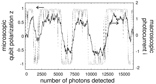
Figure 2: Microscopic and macroscopic variables.

We conclude our discussion by presenting numerical simulations of the combined effects of measurement and noise (Figs. 2 and 3). In both experiments $2^{14}=16,384$ photons are sent through the system, with phase shift $\theta=1/\sqrt{64}$. We adopt units of time such that $r=1$, hence the measurement bandwidth $r\theta^{2}/2=1/128$, so typically 128 photons suffice to measure the qubit state. The macroscopic photodiode current $i$ shown in the figures represents the photodiode current after low-pass filtering: the single-pole $RC$ filter time constant has been set to $1/(RC)=1/512$ and the zero-frequency filter gain adjusted to $1/(er\theta)$, where $e$ is the photodiode charge collected for each detected photon, such that currents of $i=\pm 1$ are expected for qubit polarization $z=\pm 1$. The noise fluctuations evident in the measured current are wholly due to photodiode shot noise. The spectral density of the Langevin noise is adjusted such that $S_{x}+S_{y}=1/2048$; thus a mean of eight transitions are expected in the course of each experiment, prior to taking the Quantum Zeno effect into account.

Fig. 2 illustrates a typical simulation. The effects of diffusion and drift velocity in the Fokker-Planck equation (Eq. 19) are readily evident in the microscopic qubit polarization — $z(t)$ does not linger near $z\sim 0$, but rather is swiftly drawn to values of $z\sim\pm 1$. Conversely, for values of $z(t)$ near $\pm 1$, Langevin noise generates numerous tunneling attempts of which only a small fraction succeed, in accord with both the Fokker-Planck and optical Bloch equations. Transitions in the macroscopic photocurrent lag behind those of the microscopic variable $z$ due to the causal nature of the low-pass filter. The transitions in Fig. 2 are induced by broad-band Langevin noise, with $\alpha=1/16$, such that the predicted Quantum Zeno suppression factor is $\alpha/(\alpha+r\theta^{2}/2)=8/9$ — essentially negligible.

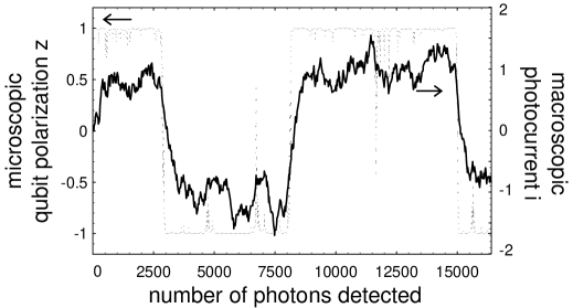
Figure 3: The Quantum Zeno effect.

Fig. 3 shows a simulation in which the Langevin noise has the same spectral density as Fig. 2, but is narrow-band, $\alpha=1/256$, such that the Quantum Zeno suppression factor is $\alpha/(\alpha+r\theta^{2}/2)=1/3$. The predicted three-fold suppression of noise-induced transitions is readily evident in $z(t)$, not only in the reduced number of outright transitions (from eight to three), but also in the reduced number and intensity of tunneling attempts.

We note that the interferometric Quantum Zeno effect discussed in the present article differs substantially from the Quantum Zeno effect experimentally observed by Itano et. al. [4], as reviewed by Wineland et. al. [10]. One major difference is that interferometric techniques probe two-state qubit systems, in contrast to the three-state ion systems of Itano et. al.. Furthermore, interferometric qubit-photon interactions are off-resonance and weak, and do not induce state transitions, while in the experiments of Itano et. al. the ion-photon interactions were on-resonance and strong, and did induce state transitions. Similarly, the quantum jumps visible in Figs. 2 and 3 are visually similar to the three-state quantum jumps experimentally demonstrated by Dehmelt [2], but differ substantially in their underlying mechanism.

The intimate relation between the AC Stark, Stern-Gerlach, and Quantum Zeno effects has not previously been described in the literature — all three effects can be predicted from knowledge of the photon flux $r$, the optical scattering phase $\theta$, and the fluctuation bandwidth $\alpha$, and the observation of any one effect implies the presence of the other two.

The results presented in this article are of substantial utility in the design of interferometric experiments. As an example, let us design a trapped-ion experiment that would generate oscilloscope traces statistically identical to those of Figs. 2 and 3 — traces in which Stern-Gerlach and Quantum Zeno phenomena are readily apparent to the naked eye. We stipulate that the duration of the oscilloscope trace is to be 10 seconds, and the detected photon flux is $1.0\ \mu{\mathrm{W}}$ at a wavelength of 6800 Å, for a total of $n_{{\mathrm{exp}}}=rt=3.4\times 10^{13}$ detected photons. Only half of this optical power passes through the interaction region; the rest is carried by the reference arm of the interferometer. The low-pass filter time constant should be set to 1/32 of the trace time, i.e., $RC=0.3\ {\mathrm{sec}}$, in order to duplicate the shot-noise fluctuations evident in the oscilloscope traces of Figs. 2 and 3. The traces have a resolving power $rt\theta^{2}=256$: the designed experiment is intended to achieve the same resolving power. This implies that the target two-state ion must generate an optical phase shift of at least $\theta_{{\mathrm{exp}}}=(256/n_{{\mathrm{exp}}})^{1/2}=2.7\times 10^{-6}$ radians. The required AC Stark frequency shift is $\delta\omega=r\theta=2.8\ {\mathrm{MHz}}=5.8\times 10^{-4}\ {\mathrm{cm}}^{-1}$. If the photon flux were boosted by a factor of $10^{6}$ (to one Watt), the detectable phase shift would be reduced by a factor of $10^{-3}$ to $2.7\times 10^{-9}$ radians; this square-root scaling is characteristic of interferometric detection. The required AC Stark shift would be $r\theta=2.8\ {\mathrm{GHz}}=0.58\ {\mathrm{cm}}^{-1}$.

In practical design work, it will often be convenient to to regard the photon flux $r$ as the primary design variable, then estimate the Stark shift $\delta\omega$ from the optical field intensity in the interaction region and the optical properties of the ion under investigation. The scattering phase $\theta$ can then be determined simply from $\theta=\delta\omega/r$.

It is beyond the scope of this article to evaluate the photon fluxes and Stark shifts that are practically achievable in trapped ion experiments; our concern is to provide specific design targets which contemplated experiments must meet.

For the benefit of students new to quantum mechanics, we remark that introductory textbooks often contain simplified or axiomatic descriptions of measurement processes which sometimes lend an unnecessarily paradoxical aspect to well-understood phenomena like the Stern-Gerlach effect. The results presented in this article are in accord with an increasingly dominant modern view — but a view requiring substantially more complicated calculations than are typically included in introductory texts — in which measurement processes work gently and incrementally to create correlations between macroscopic variables (like photodiode charge $q$) and microscopic variables (like qubit polarization $z$). At the end of an interferometric qubit measurement, all but an exponentially small fraction of data records agree that the Stern-Gerlach effect is present, but it is both unnecessary and impossible, even in principle, to identify a specific moment at which the qubit wave function collapsed. Students should also be aware that the extra work entailed in a detailed quantum measurement analysis can yield worthwhile physical insights. For example, students may reflect on our finding that spontaneous emission into a broad continuum of states is not subject to the Quantum Zeno effect — this greatly simplifies the calculation of atomic transition rates in photon-rich environments like stellar interiors, where Quantum Zeno suppression would otherwise be a large effect.

Students should also be aware that the level of detail in the analysis of quantum measurement processes is limited mainly by space considerations and by the energies of the investigator and the reader. For example, we have not specified what happens inside the photodiodes of Fig. 1, but there is no reason to think that a more detailed description of these photodiodes would change our conclusions regarding the AC Stark, Stern-Gerlach, and Quantum Zeno effects.

The results of this article can be extended in several directions. We have considered the measurement of a single qubit, yet the design of practical quantum computers will require simultaneous interferometric measurements on multiple correlated qubits [3]: the detailed theoretical analysis of this measurement process remains to be done. Single-spin magnetic resonance force microscopy (MRFM) [6, 8] is based on the interferometric measurement of a harmonic oscillator that is coupled to a two-state spin system. Stern-Gerlach phenomena are predicted to occur [7], but as yet there has been no quantum measurement analysis of this more complex interferometer-oscillator-spin system. The results of the present article were derived as a preliminary step toward a quantum measurement analysis of single-spin MRFM.

Qubit interferometry readily lends itself to delayed-choice experiments, which have yet to be analyzed in detail. We imagine, for example, that the $2\times 2$ optical coupler of Fig. 1 is separated from the interaction region by 150 kilometers of optical fiber, yielding a full millisecond of time delay in the measurement process — such delays are perfectly feasible from a technical point of view. We launch a microsecond-long pulse of $n_{{\mathrm{exp}}}\sim 10^{13}$ photons into the apparatus. After the photons have interacted with the qubit, but before they have entered the $2\times 2$ coupler, we choose whether or not to insert the coupler in the system. This delayed choice retrospectively alters the quantum state of the qubit, as per Eq. 12 with $rt=n_{{\mathrm{exp}}}$. To avoid the possibility of a backwards-in-time causality violation, the alteraction of the qubit state consequent to the delayed choice must be undetectable. In the special case that Langevin noise is absent, it can be shown from Eq. 10 that the retrospective qubit state alteraction has no detectable consequences, but a general proof that all delayed-choice qubit interferometry experiments respect causality has not yet been given.

Interesting phenomena — as yet poorly understood — occur when the condition $[A,B]=0$ is relaxed. Physically speaking, this occurs when a feedback loop is installed, such that a unitary transform $U_{a}$ is applied to the qubit whenever an A-channel photon is detected, while a (possibly different) unitary transform $U_{b}$ is applied whenever a B-channel photon is detected. Then Eqs. 1–6 still apply, with the substitutions

$$A\rightarrow A^{\prime} \!\!\equiv\!\! U_{a}A\,,$$

$$B\rightarrow B^{\prime} \!\!\equiv\!\! U_{b}B\,.$$ (37)

In general $[A^{\prime},B^{\prime}]\neq 0$. As every experimentalist knows, feedback effects often are generated inadvertently, particularly in newly-designed experiments, and the result is typically — but not invariably — noisy or chaotic behavior of the device. The author has conducted numerical experiments which support this expectation. Depending on the particular choice of $U_{a}$ and $U_{b}$, plots of the macroscopic variable $q$ and the microscopic variable $z$ show a variety of behaviors, ranging from seemingly complete randomness to complex trajectories reminiscent of chaotic attractors. However, $U_{a}$ and $U_{b}$ together span a six-dimensional parameter space which is too large for efficient empirical exploration. We therefore close by noting that Eqs. 1–6 provide a well-posed framework for investigating noisy and chaotic behaviour in the context of quantum measurement theory. From a practical point of view, the theory of noisy and chaotic devices is surely even more interesting than the theory of well-behaved devices.

References

- [1] A. Barchielli and J. Belavkin. Measurements continuous in time and a posteriori sets. Journal of Physics A, 24:1495–1513, 1991.
- [2] H. Dehmelt. Experiments with an isolated subatomic particle at rest. Reviews of Modern Physics, 62(3):525–30, 1990.
- [3] D. P. DiVincenzo. Quantum computation. Science, 270(5234):255–61, 1995.
- [4] W. M. Itano, D. J. Heinzen, J. J. Bollinger, and D. J.Wineland. Quantum zeno effect. Physical Review A, 41(5):2295–300, 1990.
- [5] D. Rugar, H. J. Mamin, and P. Guethner. Improved fiber-optic interferometer for atomic force microscopy. Applied Physics Letters, 55(25):2588–90, 1989.
- [6] J. A. Sidles. Noninductive detection of single-proton magnetic resonance. Applied Physics Letters, 58(24):2854–6, 1991.
- [7] J. A. Sidles. Folded Stern-Gerlach experiment as a means for detecting nuclear magnetic resonance in individual nuclei. Physical Review Letters, 68(8):1124–7, 1992.
- [8] J. A. Sidles, J. L. Garbini, K. J. Bruland, D. Rugar, O. Züger, S. Hoen, and C. S. Yannoni. Magnetic resonance force microscopy. Reviews of Modern Physics, 67(1):249–265, 1995.
- [9] M. Weissbluth. Photon-Atom Interactions. Academic Press, Inc., New York, 1989. For students, this text provides a concise introduction to the theoretical methods used in this article. See particularly Section 1.5 with respect to Fokker-Plank equations, 6.1 with respect to Langevin noise, 6.4 with respect to optical Bloch equations, and 6.9 with respect to spontaneous emission processes.
- [10] D. J. Wineland, J. C. Bergquist, J. J. Bollinger, and W. M. Itano. Quantum effects in measurements on trapped ions. Physica Scripta T, 59:286–93, 1995.
- [11] W. K. Wootters and W. H. Zurek. A single quantum cannot be cloned. Nature, 299(5886):802–3, 1982.
Acknowledgments
This research was supported by the University of Washington Department of Orthopædics, the NIH Biomedical Research Technology Area, the Army Research Office, and the NSF Instrument Development Program.