Abstract

Pólya states of single mode radiation field are proposed and their algebraic characterization and nonclassical properties are investigated. They degenerate to the binomial (atomic coherent) and negative binomial (Perelomov’s su(1,1) coherent) states in two different limits and further to the number, the ordinary coherent and Susskind-Glogower phase states. The algebra involved turn out to be a two-parameter deformation of both su(2) and su(1,1). Nonclassical properties are investigated in detail.

1 Introduction

Since Stoler et al. introduced the binomial states in 1985 [1], the so-called intermediate states have attracted attentions. An important feature of these states is that they interpolate between two fundamental states, such as the number, the coherent and squeezed and the phase states, and reduce to them in two different limits. For example, the binomial states (BS) [1, 2] between the number and the coherent states; the negative binomial states (NBS) [3] between the coherent and the Susskind-Glogower (SG) phase states [4]; the hypergeometric states (HGS) between the number and the coherent states [5]; the intermediate number-squeezed states [6, 7] and the intermediate number-phase states [8]. Another feature of some intermediate states is that their photon distributions are some famous probability distributions in probability theory. BS corresponds to the binomial distribution [1], NBS to the negative binomial distribution [3] and HGS to the hypergeometric distribution [5].

In this letter we shall introduce the Pólya states (PS) in the same way as the BS from the binomial distribution [9], namely, we define the Pólya states as probability amplitudes of the Pólya distribution. We find that, as intermediate states, PS interpolate between the BS and NBS, or in other words, the atomic coherent states and the Perelomov’s su(1,1) coherent states. Furthermore, the PS tend to the number and the coherent states (from BS) and the coherent and the SG phase states (from NBS). So the present letter supplies a unified approach to these important quantum states in quantum optics. As in the cases of BS and NBS, the PS also admit the ladder-operator formalism and the algebra involved is a two-parameter deformation of Holstein-Primakoff (HP) realization of both su(2) and su(1,1) in the sense that it contracts to their universal enveloping algebras in two different limits. As far as I know, this kind of deformed algebras has not appeared in the literature. The nonclassical properties of PS are also investigated. The field in PS is of sub-Poissonian and squeezed in some ranges of parameters involved.

2 Pólya states and their limiting states

We define the Pólya states as

$$|M,\gamma,\eta\rangle=\sum_{n=0}^{M}[P_{n}^{M}(\gamma,\eta)]^{1\over 2}|n\rangle,$$ (2.1)

where $|n\rangle$ is the number state of a single mode radiation field

$$[a,\,a^{\dagger}]=1,\ \ \ N\equiv a^{\dagger}a,\ \ \ a|0\rangle=N|0\rangle=0,\ \ \ |n\rangle=\frac{a^{\dagger n}}{\sqrt{n!}}|0\rangle.$$ (2.2)

$M$ is a positive integer, $\gamma>0$ is a real constant, $\eta$ is the probability satisfying $0<\eta<1$ and the photon distribution $|\langle n|M,\gamma,\eta\rangle|^{2}\equiv P_{n}^{M}(\gamma,\eta)$ is the Pólya distribution in probability theory ($\bar{\eta}=1-\eta$) [9]

$$P_{n}^{M}(\gamma,\eta)=\left(\begin{array}[]{c}M\\ n\end{array}\right)\frac{\eta(\eta+\gamma)\cdots(\eta+(n-1)\gamma)\,\bar{\eta}(\bar{\eta}+\gamma)\cdots(\bar{\eta}+(M-n-1)\gamma)}{(1+\gamma)(1+2\gamma)\cdots(1+(M-1)\gamma)}.$$ (2.3)

The Pólya states defined above is obviously normalized since as a probability distribution $P_{n}^{M}(\gamma,\eta)$ satisfies $\sum_{n=0}^{M}P_{n}^{M}(\gamma,\eta)=1$.

It is well known that the Pólya distribution tends to the binomial and negative binomial distributions in the limit $\gamma\to 0$ ( called the BS limit, for convenience) and $M\to\infty,\gamma\to 0,\eta\to 0$ with $M\eta=\lambda$ and $M\gamma=\rho^{-1}$ (called the NBS limit), respectively [9]

$$P_{n}^{M}\to\left\{\begin{array}[]{ll}\left(\begin{array}[]{c}M\\ n\end{array}\right)\eta^{n}(1-\eta)^{M-n},&\mbox{in the BS limit,}\\ \left(\begin{array}[]{c}\lambda\rho+n-1\\ n\end{array}\right)\left(\displaystyle 1-\frac{1}{1+\rho}\right)^{\lambda\rho}\left(\displaystyle\frac{1}{1+\rho}\right)^{n},&\mbox{in the NBS limit.}\end{array}\right.$$

Accordingly the PS go to the BS and NBS in the BS and NBS limits, respectively. Furthermore, the BS degenerate to the number and coherent states in two different limits [1] and the NBS to the coherent and SG phase states in two different limits [3]. So the PS include the number, the coherent states and SG phase states as their limiting states. Therefore, the PS interpolate between the BS and NBS, or in other words, between the atomic coherent states and Perelomov’s su(1,1) coherent states.

3 Algebraic Characterization

Both BS and NBS admit the ladder-operator description, namely, they satisfy the eigenvalue equations of generators of su(2) or su(1,1), respectively. In fact, the PS admit the ladder-operator description, too. It is easy to verify that PS satisfy the following eigenvalue equation

$$\gamma\left[(M-N)\left(\frac{\bar{\eta}}{\gamma}+M-N-1\right)\left(\frac{\eta}{\gamma}+N\right)\right]^{1\over 2}a|M,\gamma,\eta\rangle=\gamma(M-N)\left(\frac{\eta}{\gamma}+N\right)|M,\gamma,\eta\rangle.$$ (3.1)

Then in the BS or NBS limits, (3.1) tend to the ladder-operator forms of BS and NBS

$$\sqrt{1-\eta}J^{-}_{M}|M,0,\eta\rangle=\sqrt{\eta}(M-N)|M,0,\eta\rangle,\ \ \ J^{-}_{M}\equiv\sqrt{M-N}\,a,$$ (3.2)

$$\sqrt{\rho+1}K^{-}_{\lambda\rho}|\infty,0,0\rangle=(\lambda\rho+N)|\infty,0,0\rangle,\ \ \ K^{-}_{\lambda\rho}\equiv\sqrt{\lambda\rho+N}\,a,$$ (3.3)

where $J^{-}_{M}$ and $K^{-}_{\lambda\rho}$ are the lowering operators of su(2) and su(1,1) algebras via their HP realizations. Both limiting results (3.2, 3.3) suggest us defining the operator on the left side of (3.1) as the lowering operator (up to a constant) of the algebra related to PS

$$A^{-}=\frac{\gamma}{\sqrt{(1-\eta)(1+M\gamma)(M\gamma+\eta)}}\left[(M-N)\left(\frac{\bar{\eta}}{\gamma}+M-N-1\right)\left(\frac{\eta}{\gamma}+N\right)\right]^{1\over 2}a.$$ (3.4)

Then the algebraic relations among $A^{-}$, the raising operator $A^{+}\equiv(A^{-})^{\dagger}$ and $N$ are obtained as

$$[N,\,A^{\pm}]=\pm A^{\pm},\ \ \ \ A^{+}A^{-}=F(N),\ \ \ \ A^{-}A^{+}=F(N+1),$$ (3.5)

where $F(N)$ is a non-negative hermitian function

$$F(N)=\frac{N(M-N+1)(\bar{\eta}+\gamma M-\gamma N)(\eta+\gamma N-\gamma)}{(1-\eta)(\gamma M+1)(\gamma M+\eta)}.$$ (3.6)

This means that the related algebra, which is an associative algebra generated by $A^{-}$, $A^{+}$, $N$ and the unit 1, is a generally deformed oscillator with the structure function $F(N)$. This algebra has an $(M+1)$-dimensional representation on the Fock space because of the condition $A^{+}|M\rangle=F(M+1)|M+1\rangle=0$.

A remarkable feature of this algebra is that in the BS and NBS limits it contracts to the universal enveloping algebras of compact su(2) and noncompact su(1,1) Lie algebra:

$$A^{-}\longrightarrow\left\{\begin{array}[]{ll}\sqrt{M-N}a\equiv J^{-}_{M}&\mbox{in the BS limit,}\\ \sqrt{\lambda\rho+N}a\equiv K^{-}_{\lambda\rho}&\mbox{in the NBS limit.}\end{array}\right.$$ (3.7)

Accordingly, its finite dimensional representation degenerates to a finite dimensional irreducible representation of su(2) with the highest weight $M/2$ and the infinite dimensional irreducible positive discrete representation of su(1,1) with the Bargmann index $\lambda\rho/2$.

4 Nonclassical Properties

4.1 Photon Statistics

The averages $\langle N\rangle$, $\langle N^{2}\rangle$ and fluctuation $\langle\Delta N^{2}\rangle$ are obtained as

$$\langle N\rangle=M\eta,\ \ \ \langle N^{2}\rangle=M\eta+\frac{M\eta(M-1)(\eta+\gamma)}{1+\gamma},\ \ \ \langle\Delta N^{2}\rangle=\frac{M\eta(M\eta+1)(1-\eta)}{1+\gamma},$$ (4.1)

Then we can easily derive Mandel’s $Q$-factor

$$Q^{M}_{\gamma}(\eta)=\frac{\langle\Delta N^{2}\rangle-\langle N\rangle}{\langle N\rangle}=\frac{(M-1)\gamma}{1+\gamma}-\eta\frac{M\gamma+1}{1+\gamma},$$ (4.2)

which is obviously a linear function of $\eta$ and is a straight line (we call it the $Q$-line for convenience) connecting the point $\left(0,Q_{\gamma}^{M}(0)\right)$ and $\left(1,Q_{\gamma}^{M}(1)\right)$, where

$$Q_{\gamma}^{M}(0)=\frac{(M-1)\gamma}{1+\gamma}\equiv(M-1)\left(1-\frac{1}{1+\gamma}\right),\ \ \ \ Q_{\gamma}^{M}(1)=-1,$$ (4.3)

as illustrated in the Figure 1. We find that

1. In the case $M=1$ or $\gamma=0$ (BS limit), we have $Q_{\gamma}^{M}(0)=0$ and the $Q$-line connects (0,0) and $(1,-1)$. So in this case $Q_{\gamma}^{M}(\eta)=-\eta<0$ and the field is of sub-Poissonian character except for $\eta=0$, which corresponds to the Poissonian statistics.

2. If $\gamma>0$ and $M\neq 1$, then $Q_{\gamma}^{M}(0)>0$ and the $Q$-line must intersect with the line $Q_{\gamma}^{M}(\eta)=0$ at the point

$$\left(\frac{(M-1)\gamma}{M\gamma+1},\,0\right)$$ (4.4)

(see Fig.1). This means that, when $\eta>\frac{(M-1)\gamma}{M\gamma+1}$ (or $\eta<\frac{(M-1)\gamma}{M\gamma+1}$ ), $Q_{\gamma}^{M}(\eta)<0$ (or $Q_{\gamma}^{M}(\eta)>0$) and the field in PS is of sub-Poissonian (super-Poissonian). The point $\eta=\frac{(M-1)\gamma}{M\gamma+1}$ corresponds to the Poissonian statistics. In this case, the value of $M$ and $\eta$ will affect the ranges of sub-Poissonian (or super-Poissonian) statistics. The larger $M$ or/and $\gamma$, the larger $Q_{\gamma}^{M}(0$) and therefore $\frac{(M-1)\gamma}{M\gamma+1}$. So the sub-Poissonian range $\frac{(M-1)\gamma}{M\gamma+1}<\eta<1$ becomes smaller.

4.2 Squeezing Effect

It is easy to evaluate that

$$a^{k}|M,\gamma,\eta\rangle=\left[\prod_{i=0}^{k-1}(M-i)\frac{k\gamma+\eta}{k\gamma+1}\right]^{1\over 2}\left|M-k,\frac{\gamma}{k\gamma+1},\frac{k\gamma+\eta}{k\gamma+1}\right\rangle,$$ (4.5)

for $k\leq M$ and $a^{k}|M,\gamma,\eta\rangle=0$ for $k>M$. Define the coordinate $x$ and the momentum $p$ as

$$x=\frac{1}{\sqrt{2}}(a^{\dagger}+a),\ \ \ \ p=\frac{i}{\sqrt{2}}(a^{\dagger}-a).$$ (4.6)

Then their variances are obtained as

$$\langle\Delta x^{2}\rangle = \frac{1}{2}+M\eta+\left[{M\eta(M-1)\frac{\eta+\gamma}{\gamma+1}}\right]^{1\over 2}\sum_{n=0}^{M-2}\sqrt{P_{n}^{M}(\gamma,\eta)P_{n}^{M-2}\left(\frac{\gamma}{2\gamma+1},\frac{2\gamma+\eta}{2\gamma+1}\right)}$$ (4.7)

$$-2M\eta\left[\sum_{n=0}^{M-1}\sqrt{P_{n}^{M}(\gamma,\eta)P_{n}^{M-1}\left(\frac{\gamma}{\gamma+1},\frac{\gamma+\eta}{\gamma+1}\right)}\right]^{2},$$

$$\langle\Delta p^{2}\rangle = \frac{1}{2}+M\eta-\left[{M\eta(M-1)\frac{\eta+\gamma}{\gamma+1}}\right]^{1\over 2}\sum_{n=0}^{M-2}\sqrt{P_{n}^{M}(\gamma,\eta)P_{n}^{M-2}\left(\frac{\gamma}{2\gamma+1},\frac{2\gamma+\eta}{2\gamma+1}\right)}.$$ (4.8)

Figures 2 and 3 are plots showing how $\langle\Delta x^{2}\rangle$ and $\langle\Delta p^{2}\rangle$ depend on the parameter $\gamma$ and $\eta$, respectively. In each case, different values of $M$ (5 and 20) are chosen. From these plots we find that:

Quadrature $x$ (see Fig.2). When $\gamma=0$ (BS case), the quadrature $x$ is squeezed in a considerable range $0<\eta\leq\eta_{0}<1$ of values of $\eta$, with a maximum of squeezing (minimum of $\langle\Delta x^{2}\rangle$ that depends on $M$ (the larger $M$, the wider the range and the smaller $\langle\Delta x^{2}\rangle$), as indicated in [1] and Fig.2. With the increase of $\gamma$, the squeezing range becomes smaller and smaller and $\langle\Delta x^{2}\rangle$ becomes larger and larger until the squeezing disappears for large enough $\gamma$. For large $M$, the squeezing disappears faster than that for small $M$.

Quadrature $p$ (see Fig.3). It is well known that there is no squeezing for $\gamma=0$ (BS). However, with the increase of $\gamma$, the quadrature $p$ becomes squeezed drastically in the range of $0<\eta\leq\eta_{0}<1$ and $|\langle\Delta p^{2}\rangle|$ decreases drastically until the maximum of squeezing is reached. Then, by further increasing $\gamma$, the squeezing range becomes smaller and smaller and squeezing becomes weaker and weaker. However, the quadrature $p$ is still squeezed for a very large value of $\gamma$. In fact, we can check that only when $\gamma\to\infty$, $\langle\Delta p^{2}\rangle$ goes to $1/2$. We also see that $\langle\Delta p^{2}\rangle$ for large $M$ is more sensitive to the parameter $\gamma$ than that for small $M$.

5 Conclusion

In this letter we have introduced and investigated the Pólya states and found that:

1. As intermediate states, the Pólya states interpolate the binomial states (or the atomic states) and the negative binomial states (or the Perelomov’s coherent states).

2. Ladder-operator forms of BS and NBS, which are related to su(2) and su(1,1) algebras respectively, are generalized to the PS case. This algebraic characterization leads to an algebra which is a two-parameter ($\eta$ and $\gamma$) deformation of universal enveloping algebra of Lie algebras su(2) and su(1,1) and contracts to them in two different limits. This is natural since the PS is an intermediate state between su(2) (BS) and su(1,1) (NBS) coherent states. To our knowledge this kind of algebras which mixes su(2) and its noncompact counterpart su(1,1) has not appeared before in the literature.

3. We have indicated in [3] that the nonclassical properties of BS and NBS are complementary. As states interpolating the BS and NBS the PS clearly share the characters of both BS and NBS: the field in PS is of sub-Poissonian character in some range of parameters involved and of super-Poissonian character in a different region of parameters, and both quadratures $x$ and $p$ are squeezed in considerable ranges of parameters.

Appendix: The Pólya distribution

Pólya originally introduced the Pólya distribution in 1930 [10] when considering the sampling from a finite population of objects, the numbers of which change with the removal of each individual unit. Suppose an urn contains $a$ white balls and $b$ black balls. A ball is chosen at random and replaced, together with $c$ balls of the same kind. If $M$ successive drawing have already been made, of which $n$ are white and $M-n$ black, the probability $P_{n}$ of obtaining $n$ white balls in a sequence of $M$ is

$$P_{n}=\left(\!\!\!\begin{array}[]{c}M\\ n\end{array}\!\!\!\right)\frac{a(a+c)\cdots[a+c(n-1)]b(b+c)\cdots[b+c(M-n-1)]}{(a+b)(a+b+c)\cdots[a+b+c(M-1)]}.$$

This is just the Pólya distribution (2.3) if we put

$$\eta=\frac{a}{a+b},\ \ \ \ \ \bar{\eta}=\frac{b}{a+b},\ \ \ \ \ \gamma=\frac{c}{a+b}.$$

For more details please see [9].

Figure 1: The Mandel’s $Q$-factor $Q_{\gamma}^{M}(\eta)$ as a linear funtion of $\eta$. This line is from $\left(0,\frac{(M-1)\gamma}{1+\gamma}\right)$ to $(1,-1)$.

         

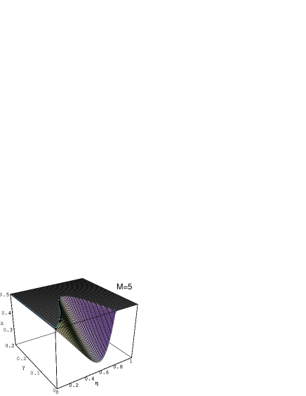
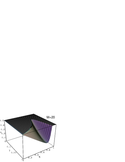
Figure 2: Variance $\langle\Delta x^{2}\rangle\equiv X$ as a function of $\eta$ and $\gamma$ for $M=5,\,20$.

         

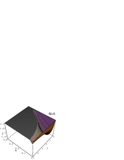
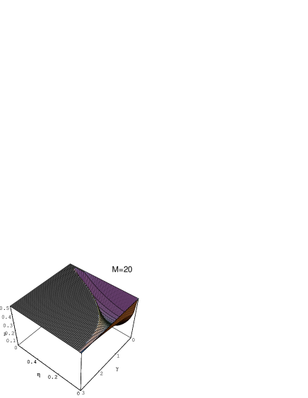
Figure 3: Variance $\langle\Delta p^{2}\rangle\equiv P$ as a function of $\eta$ and $\gamma$ for $M=5,\,20$.

References

- [1] Stoler D, Saleh B E A and Teich M C 1985 Opt. Acta. 32, 345
- [2] Vidiella-Barranco A and Roversi J 1994 Phys. Rev. 50A 5233
-
[3]
Fu H C and Sasaki R 1996 Negative Binomial and
Multinomial States: probability distributions and
coherent states quant-ph/9610022;
Fu H C and Sasaki R 1996 Negative Binomial States of quantized radiation fields quant-ph/9610024 - [4] Susskind L and Glogower J 1964 Physics 1 49
- [5] Fu H C and Sasaki R 1996 Hypergeometric states and their nonclassical properties quant-ph/9610021
- [6] Baseia B, de Lima A F and de Silva A J 1995 Mod. Phys. Lett. 9A 1673
- [7] Fu H C and Sasaki R 1996 J. Phys. 29A 5637
- [8] Baseia B, de Lima A F and Marques G C 1995 Phys. Lett. 204A 1
- [9] Moran P A P 1968 An Introduction to probability theory (Oxford Science Publications)
- [10] Pólya G 1930 Annls Inst. h. Poincaré. 1 117