Deconstructing Decoherence

Abstract

The study of environmentally induced superselection and of the process of decoherence was originally motivated by the search for the emergence of classical behavior out of the quantum substrate, in the macroscopic limit[1]. This limit, and other simplifying assumptions, have allowed the derivation of several simple results characterizing the onset of environmentally induced superselection; but these results are increasingly often regarded as a complete phenomenological characterization of decoherence in any regime. This is not necessarily the case: The examples presented in this paper counteract this impression by violating several of the simple “rules of thumb”. This is relevant because decoherence is now beginning to be tested experimentally[2, 3], and one may anticipate that, in at least some of the proposed applications (e.g., quantum computers), only the basic principle of “monitoring by the environment”[1] will survive. The phenomenology of decoherence may turn out to be significantly different.

2

I Introduction

According to deconstructionist philosophers, words refer only to other words. There is a certain amount of truth in the analogous suggestion that papers in theoretical physics refer only to other papers (and quite often, only to other papers in theoretical physics). Consequently, a term like “decoherence” is in real danger of coming to mean, to most physicists, only the processes that have been most frequently studied in the literature. Most of this literature has heretofore dealt, naturally enough, with highly idealized models amenable to exact solution. Moreover, many of these models have been particularly designed to realize a macroscopic classical limit, in order to attain the original goal of understanding the quantum origins of classicality. Such models have provided a relatively small set of principles, which could easily be taken to govern decoherence in general. It is tempting, for example, to quote a simple formula derived from a linear model[4, 5] as giving “the” decoherence timescale[6]. Emblematic of this problem is a well-known cartoon that appears in introductory discussions of decoherence[7], depicting a border crossing between the two realms of classical and quantum physics. While this is a provocative metaphor, it may prompt the inaccurate impression that there is exactly one well-defined way of crossing from one realm to the other.

In this paper we will effectively argue that many perceived universalities in the phenomenology of decoherence are artifacts of studying toy models, and that the single neat border checkpoint should be replaced as an image for decoherence by the picture of a wide and ambiguous No Man’s Land, filled with pits and mines, which may be crossed on a great variety of more or less tortuous routes. Once one has indeed crossed this region, and travelled some distance away from it, the going becomes easier: we are not casting doubt on the ability of the very strong decoherence acting on macroscopic objects to enforce effective classicality. But in the near future precise experiments (for example, [3, 2, 8, 9, 10, 11, 12, 13]) will explore regimes in which decoherence should be measurable, but not so strong as simply to enforce classicality. Experiment is thus beginning to probe the quantum/classical No Man’s Land itself, advancing daring patrols along an impressively broad front. In comparing the results of these experiments with theoretical predictions, it will be important not to assume that the simple cases examined so far should be taken as representative of decoherence in general. By presenting a number of theoretically tractable examples in which various elements of phenomenological lore can be seen to fail explicitly, we make the point that each experimental scenario will have to be examined theoretically on its own merits, and from first principles.

From the bulk of previous theoretical studies of decoherence, one might be tempted to deduce three significant principles concerning the rate of decoherence: one can define a simple decoherence time scale which is valid at least for linear systems at high temperature; the rate of decoherence of classically impossible “Schrödinger’s Cat” states is always set by the fastest time scales present; and the rate of decoherence increases with the square of the distance between the two branches of such Cat states. These elements of the standard lore are indeed borne out in the results of the first decoherence experiment at hand[3]; but there is no guarantee that they will always hold. We therefore show why in the most general mesoscopic regime one may need to go back to the basic idea that the environment “monitors” an open quantum system[1], and from there derive phenomenology afresh for every model. We will consider the three putative principles in successive sections, presenting in each section an explicit example in which the property determined for simple models previously studied no longer holds. A final section will then discuss our results collectively, and suggest some implications of them for the interpretation of experiments currently proposed or in progress.

II Decoherence timescale in linear Brownian motion

Many studies of decoherence have involved completely linear models, in which a single Brownian particle is placed in a quadratic potential, and coupled linearly to a heat bath composed of (often, uncountably many) harmonic oscillators. It can in fact be argued[14] that environments with non-linear internal dynamics can often be closely approximated, as far as their effects on the observed system are concerned, by such an independent oscillator model. Although there are certainly cases in which it is not realistic, the independent oscillator model is therefore not entirely a toy, and represents a simplicity that is actually realized in nature. And simple as it is, even it is not really simple as special cases and convenient approximations often make it appear.

The canonical example of decoherence is the evolution of a Brownian harmonic oscillator from an initial state which is a superposition of two coherent states localized at distinct positions in space. This initially pure state, assumed to be uncorrelated with the initial thermal state of an independent oscillator environment, has been found to evolve rapidly into an incoherent mixture of the two coherent states. Simple formulas are often applied to quantify “rapidly”. Here, however, we will present an easy derivation of the short-time behaviour of the Wigner function for an Ohmic Brownian oscillator, and show that there is in general no natural way to identify a single time scale for decoherence, even in the high temperature limit. Our more explicit results are in agreement with the physical conclusions reached on the basis of numerical evidence in Reference [16].

For our completely linear model, we take the Hamiltonian

$$H = {1\over 2M}P^{2}+{M\Omega^{2}\over 2}Q^{2}$$ (2)

$$\;+{1\over 2}\int_{0}^{\infty}\!d\omega\,[(p_{\omega}+gf_{\omega}Q)^{2}+\omega^{2}q_{\omega}^{2}]\;,$$

where $P$ and $Q$ are the Brownian particle’s canonical variables, and $M$ and $\Omega$ are its mass and natural frequency; $p_{\omega}$ and $q_{\omega}$ are the canonical variables for the bath oscillator with frequency $\omega$; $g$ is an overall coupling strength which may be used to define the dissipation rate

$$\gamma\equiv{\pi g^{2}\over 4M}\;;$$ (3)

and $f_{\omega}$ describes the relative coupling strength of the various environmental modes. The square of this strength will play the role of a spectral density.

The initial Wigner function $W(Q,P;0)$ of the Brownian oscillator will be that for an equal amplitude superposition of two coherent states, whose wave functions are Gaussians displaced equal and opposite amounts $\pm a$ from the origin. This Wigner function contains two terms, then: one consisting of a sum of two Gaussians, representing the incoherent mixture of the two states; and one which is oscillatory, and represents their quantum interference:

$$W(Q,P;0) = W_{mix}+W_{int}$$ (4)

$$W_{mix}(Q,P;0) = {(1-e^{-M\Omega a^{2}/\hbar})^{-1}\over\pi\hbar}\cosh\Bigl{(}2{M\Omega\over\hbar}aQ\Bigr{)}$$ (6)

$$\times\exp\Bigl{[}-{1\over\hbar\Omega}\Bigl{(}{P^{2}\over M}+M\Omega^{2}(Q^{2}+a^{2})\Bigr{)}\Bigr{]}$$

$$W_{int}(Q,P;0) = {(1-e^{-M\Omega a^{2}/\hbar})^{-1}\over\pi\hbar}\cos\Bigl{(}2{aP\over\hbar}\Bigr{)}$$ (8)

$$\times\exp\Bigl{[}-{1\over\hbar\Omega}\Bigl{(}{P^{2}\over M}+M\Omega^{2}Q^{2}\Bigr{)}\Bigr{]}\;.$$

Decoherence in this model appears as a rapid decay in magnitude of $W_{int}(Q,P;t)$, by means of an exponential prefactor $e^{-D(t)}$.

The initial Wigner function for the complete system of Brownian oscillator plus bath is assumed to be a direct product

$${\cal W}(Q,P;\{q_{\omega},p_{\omega}\};0)=W(Q,P;0)\times W_{e}[q_{\omega},p_{\omega}]$$ (11)

$$W_{e}[q_{\omega},p_{\omega}]=\prod_{\omega}{\tanh(\hbar\beta\omega/2)\over\pi\hbar}$$

$$\qquad\qquad\times\exp\Bigl{[}-{1\over\hbar\omega}(p^{2}_{\omega}+\omega^{2}q^{2}_{\omega})\tanh{\hbar\beta\omega\over 2}\Bigr{]}\;,$$

where $\beta=(k_{B}T)^{-1}$ is the inverse temperature of the environment.

It can be shown quite easily that the Wigner function for a totally linear system evolves under the same Liouville equation as the classical ensemble density for the same model. Consequently, we can evolve the Wigner function by simply propagating it along the classical trajectories in phase space. The reduced Wigner function for the Brownian particle alone, with the environment integrated out, is therefore

$$W(Q_{F},P_{F};t_{F})$$ (12)

$$= \int\!dQ_{I}dP_{I}{\cal D}q_{\omega I}{\cal D}p_{\omega I}\,\delta\bigl{(}Q_{F}-Q_{0}(t_{F})\bigr{)}\delta\bigl{(}P_{F}-P_{0}(t_{F})\bigr{)}$$ (14)

$$\qquad\times W(Q_{I},P_{I};0)W_{e}[q_{\omega I},p_{\omega I}]$$

$$= \int{\cal D}q_{\omega I}{\cal D}p_{\omega I}\,\Bigg{|}{\partial(Q_{I},P_{I})\over\partial(Q_{F},P_{F})}\Bigg{|}\,W_{e}[q_{\omega I},p_{\omega I}]\,W\bigl{(}Q_{I},P_{I};0)\;,$$ (15)

where $Q_{0}(t)$ and $P_{0}(t)$ are given by Hamilton’s equations, for the Hamiltonian (2). We have simplified presentation in (12) at the expense of precise notation: in the first line, $Q_{I}$ and $P_{I}$ are dummy variables, and we implicitly assume the initial boundary conditions $Q_{0}(0)=Q_{I},P_{0}(0)=P_{I}$; but in the second line, we intend instead the final boundary conditions $Q_{0}(t)=Q_{F},P_{0}(t)=P_{F}$, and we use $Q_{I},P_{I}$ as shorthand for the resulting $Q_{0}(0),P_{0}(0)$. In the remainder of this discussion, we will continue the usage of the second line, according to which it should be noted that $Q_{I}$ and $P_{I}$ are in fact functions of the final time $t_{F}$, and linear functions of $Q_{F}$, $P_{F}$, and initial environmental variables $\{q_{\omega I},p_{\omega I}\}$.

We are interested in decoherence that occurs on time scales much shorter than the Brownian particle’s dynamical time scale $\Omega^{-1}$, and when the environment is very weakly coupled to the system. We will therefore solve the equations of motion for $Q_{0}$ and $P_{0}$ perturbatively to first order in $\Omega t$ and at most first order in $g$, to obtain

$$Q_{I}(t) \doteq Q_{F}-{P_{F}\over M}t$$ (16)

$$P_{I}(t) \doteq P_{F}+M\Omega^{2}Q_{F}t+\int_{0}^{t}\!dt^{\prime}\,F_{1}(t^{\prime})\;,$$ (17)

where $F_{1}(t)$ is the force exerted by the environment, to first order in $g$. Since this force will be a linear function of the $q_{\omega I}$ and $p_{\omega I}$, and since to form the reduced Wigner function $W(Q_{F},P_{F};t_{F})$ we will be integrating over these variables with the Gaussian weight $W_{e}$, Eqn. (16) is effectively a Langevin equation with a Gaussian stochastic force. Note also that Equation (16) implies that the Jacobian in Equation (12) is simply $1$, to first order in $\Omega t$.

There are some subtle points to be considered before writing down the expression for $F_{1}(t)$. One might be tempted simply to write $F_{1}(t)\doteq F_{1}(0)=g\int\!d\omega\,f_{\omega}p_{\omega I}$; but this would be forgetting the fact that $F_{1}(t)$ can contain some frequencies much higher than $\Omega$, so that some components of the stochastic force will oscillate significantly even over the short time interval in which we can expect to see decoherence. We therefore write the more accurate expression

$$F_{1}(t)=g\int_{0}^{\infty}\!d\omega\,f_{\omega}\,[p_{\omega I}\cos\omega t+\omega q_{\omega I}\sin\omega t]\;.$$ (18)

Actually, neglecting higher order terms in $g$ will be inaccurate, even for very early times, if the high-frequency end of the environmental spectrum is too strong. As one finds by fully solving such “supra-ohmic” models, higher order terms in $g$ can appear multiplied by large frequencies, and thus be significant. In such cases, backreaction can be so swift that a counterterm to the “bare” force $F_{1}(t)$ is generated rapidly enough to affect (and typically suppress) decoherence. One can understand this phenomenon roughly as the rapid onset of adiabatic dragging of the high frequency bath degrees of freedom; it is discussed in detail, in Reference [17].

These subtleties of backreaction turn out to be insignificant in the much-studied Ohmic case, where (for the coupling scheme we are using) $f_{\omega}$ is constant up to some high UV cut-off scale. We will therefore assume the Ohmic case, choosing for definiteness the Lorentzian cut-off scheme

$$f_{\omega}={\Gamma\over\sqrt{\omega^{2}+\Gamma^{2}}}$$ (19)

with $\Gamma>>\Omega$, and accept Equation (18) as valid. Working to first order in $\Omega t$, we find that the Brownian particle gains negligible energy from the environment at these very early times:

$${P_{I}^{2}\over M}+M\Omega^{2}Q_{I}^{2}\doteq{P_{F}^{2}\over M}+M\Omega^{2}Q_{F}^{2}\;,$$ (20)

when we neglect $g$ completely because we assume that $P_{I}\int\!dt^{\prime}\,F(t^{\prime})/M$ is negligible for the $|P_{I}|\sim\sqrt{M\hbar\Omega}$ that are significant in $W(Q_{I},P_{I};0)$. Even though the environmental force is too small to affect the energy of the Brownian particle at these early times, however, $a>>\sqrt{\hbar/M\Omega}$ will allow the change in $aP$ to be significant:

$$aP_{I} \doteq aP_{F}$$ (22)

$$\;+ag\int_{0}^{\infty}\!{d\omega\over\omega}f_{\omega}\,[p_{\omega I}\sin\omega t+\omega q_{\omega I}(1-\cos\omega t)]\;.$$

Performing the Gaussian integrals in Equation (12) using (20) and (22), we find that $W_{mix}(Q,P;t)$ is negligibly changed from $W_{mix}(Q,P;0)$, but that $W_{int}(Q,P;0)$ has evolved into

$$W_{mix}(Q,P;t)\doteq e^{-D(t)}W_{mix}(Q,P;0)\;,$$ (23)

where the decoherence factor $D(t)$ is given by

$$D(t)={8M\gamma a^{2}\over\pi\hbar}\int_{0}^{\infty}\!{d\omega\over\omega}\,f_{\omega}^{2}\coth{\hbar\beta\omega\over 2}\,(1-\cos\omega t)\;.$$ (24)

In the zero temperature limit, Equation (24) agrees with Eqns. (36)–(37) of Reference [18], which present a weak coupling, early time approximation to an exact solution once it has been obtained. In the high temperature limit, we can explicitly evaluate $D(t)$ as

$$D(t)\stackrel{{\scriptstyle\scriptscriptstyle T\to\infty}}{{\longrightarrow}}{8\gamma k_{B}Ta^{2}\over\hbar^{2}}\Bigl{(}t-{1-e^{-\Gamma t}\over\Gamma}\Bigr{)}\;.$$ (25)

For times much less than $\Omega^{-1}$ but still much greater than $\Gamma^{-1}$, Equation (25) agrees with previous results that at high temperatures $D(t)\propto t$. This linear behaviour of $D(t)$ allows one to specify a single decoherence time scale

$$\tau_{dec}={\hbar^{2}\over 8M\gamma a^{2}k_{B}T}\;.$$ (26)

Even when the high temperature limit $k_{B}T>>\hbar\Gamma$ is valid, however, this formula is not really universal. For sufficiently high $T$ or $a^{2}$, decoherence will already have occurred ($e^{-D(t)}<<1$) at times smaller than or on the order of $\Gamma^{-1}$. We will then have to write

$$D(t)\simeq{4M\gamma k_{B}Ta^{2}\over\hbar^{2}}\Gamma t^{2}\;,$$ (27)

from which one must deduce the much longer timescale

$$\tau^{\prime}_{dec}={\hbar\over 2a\sqrt{M\gamma\Gamma k_{B}T}}\;.$$ (28)

For lower temperatures, or non-Ohmic environments, $D(t)$ will generally not be linear, and the time at which $e^{-D(t)}<<1$ will be a complicated function of temperature and $a^{2}$. The existence of a single simple formula for “the” decoherence time scale is a special property of the Ohmic independent oscillator model at high, but not ultra-high, temperatures.

III Initial state preparation

Simple or not, all the decoherence timescales which might be identified in models like that of Section II have the common feature of being very short. Warnings have long been made, however, that that the rapidity of this initial burst of decoherence might be spurious, in that it might be a special consequence of an initial state in which the system and environment are negligibly entangled. Since it is the high frequency modes of the environment that are responsible for rapid decoherence, the neglect of initial entanglement is particularly dubious: these fast modes are precisely the ones which will tend to be adiabatically dragged along with the system, if the system is put into a “Schrödinger’s Cat” state by a physical process instead of by theoretical fiat. Despite warnings about this issue in prose, however, there has so far been no actual calculation to really lay this ghost to rest.

In this section we examine a model which is essentially the same as those of Section II or Reference [18]. Instead of following the evolution of an initial superposition of displaced Gaussian states, however, we will take the ground state of the complete system as our initial state, and apply an external force which drives the Brownian oscillator into a superposition of displaced Gaussians over a finite period of time. We find that decoherence occurs in this scenario, but that it is no longer characterized by the short UV time scale. The strong initial burst of decoherence, which has been ubiquitous but suspect in previous studies, is indeed suppressed.

We again take the Hamiltonian

$$H_{0} = {P^{2}\over 2M}+{M\Omega^{2}\over 2}Q^{2}$$ (30)

$$\;+{1\over 2}\int_{0}^{\infty}\!d\omega\,[(p_{\omega}+gf_{\omega}Q)^{2}+\omega^{2}q_{\omega}^{2}]\;,$$

just as in Equation (2) above. We also retain the Ohmic specification for $f_{\omega}$ given by Equation (19). We do make an important change in our system, however, even though it does not show up in $H_{0}$: we endow our Brownian oscillator with a two-state internal degree of freedom, such as a spin. The Hamiltonian as written so far does not distinguish between the oscillator’s two internal states; but we now add to it an external force which does distinguish them, and which will thereby be able to create a Schrödinger’s Cat state from the ground state:

$$H_{\alpha}=H_{0}+a\alpha(t)\hat{\sigma}{P}\;.$$ (31)

Here $a$ is again a distance scale, $\alpha(t)$ is a time-dependent c-number having dimensions of frequency, with $\alpha(0)=0$, and the Pauli spin matrix $\hat{\sigma}$ acts in the internal space. We will then take our initial state to be

$$|\Psi_{i}\rangle={1\over\sqrt{2}}|\phi_{0}\rangle\bigl{(}|+\rangle+|-\rangle\bigr{)}\;,$$ (32)

where $|\phi_{0}\rangle$ is the ground state of $H_{0}$, and $\hat{\sigma}|\pm\rangle=\sigma|\pm\rangle$ for $\sigma=\pm 1$.

Since the internal state of the oscillator does not evolve in this model, the two different realizations of $\sigma$ which are present in the initial state merely label two branches of the total quantum state at any time. For non-zero $\alpha(t)$, the spatial wave functions associated with these two branches will over time become quite different. Choosing $\alpha(t)=2\delta(t)$, for example, will reproduce the initial Schrödinger’s Cat state of Reference [18] (which is very similar to that of Section II above). In what follows here we will consider the case where $\alpha(t)$ is not a delta function.

As explained in Reference [18], $H_{0}$ can be diagonalized by defining new operators $A_{\omega},\pi^{A}_{\omega}$:

$${H}_{0}={1\over 2}\int_{0}^{\infty}\!d\omega\,\bigl{[}(\pi^{A}_{\omega})^{2}+\omega^{2}A_{\omega}^{2}\bigr{]}\;,$$ (33)

where

$${P} = \int_{0}^{\infty}\!d\omega\,p(\omega){A}_{\omega}$$ (34)

$$p(\omega) = {g\omega^{2}\Gamma\over\sqrt{\pi[\omega^{2}+\bar{\Gamma}^{2}][\omega^{2}-(\bar{\Omega}+i\bar{\gamma})^{2}][\omega^{2}-(\bar{\Omega}-i\bar{\gamma})^{2}]}}\;.$$ (35)

The barred quantities $\bar{\Gamma}$, $\bar{\Omega}$, and $\bar{\gamma}$ are renormalized versions of the bare parameters. The bare parameters may be expressed simply in terms of the renormalized ones (the inverse relation being a complicated cubic formula)[18], but we will assume that $\Gamma>>\Omega>>\gamma$, and in this case the differences between the barred and unbarred quantities are negligible. ${Q}$, ${q}_{\omega}$, and ${p}_{\omega}$ may also be expressed in terms of the new operators, but we will only be needing Eqn. (34).

Since the wave functional for the ground state $|\phi_{0}\rangle$ is the familiar harmonic oscillator Gaussian, it is easy to work out the wave functional for the state at time $t$ in the $\pi^{A}_{\omega}$ representation:

$$\Psi[\pi^{A}_{\omega},\sigma;t]$$ (36)

$$= \langle\sigma|\langle\pi_{\omega}^{A}|{\cal T}e^{-{i\over\hbar}\int_{0}^{t}\!dt^{\prime}\,{H}_{\alpha}(t^{\prime})}|\phi_{0}\rangle|\sigma\rangle$$ (37)

$$= Z(t)\exp\Bigl{[}-{1\over 2\hbar}\int_{0}^{\infty}\!{d\omega\over\omega}\,\Bigl{(}[\pi^{A}_{\omega}$$ (40)

$$\qquad+\sigma p(\omega)\int_{0}^{t}\!dt^{\prime}\,\alpha(t^{\prime})\cos\omega(t-t^{\prime})]^{2}$$

$$\qquad+2i\sigma p(\omega)\pi^{A}_{\omega}\int_{0}^{t}\!dt^{\prime}\,\alpha(t^{\prime})\sin\omega(t-t^{\prime})\Bigr{)}\Bigr{]}\;.$$

${\cal T}$ denotes time ordering, and $Z(t)$ is a normalization constant into which we have absorbed an irrelevant time-dependent phase. We can then obtain the reduced density matrix for the Brownian particle, in the $Q$ representation, merely by performing some Gaussian integrals:

$$\rho(Q,Q^{\prime},\sigma,\sigma^{\prime};t)$$ (41)

$$= \int\!d\xi\int\!{\cal D}\pi^{A}\,\exp\Bigl{[}{i\over\hbar}\xi\int_{0}^{\infty}\!d\omega{p(\omega)\over M\omega^{2}}\pi^{A}_{\omega}\Bigr{]}$$ (43)

$$\qquad\qquad\times\Psi[\pi^{A}_{\omega}-p(\omega)Q,\sigma;t]\Psi^{*}[\pi^{A}_{\omega}-p(\omega)Q^{\prime},\sigma^{\prime};t]$$

$$= N\exp\Bigl{[}-{M\Omega_{2}\over 4\hbar}\Bigl{(}{\Omega_{1}\over\Omega_{2}}[Q-Q^{\prime}$$ (49)

$$\qquad\qquad\qquad\qquad-(\sigma-\sigma^{\prime})\int_{0}^{t}\!dt^{\prime}\alpha(t^{\prime})y(t-t^{\prime})]^{2}$$

$$\qquad\qquad+[Q+Q^{\prime}-(\sigma+\sigma^{\prime})\int_{0}^{t}\!dt^{\prime}\alpha(t^{\prime})r(t-t^{\prime})]^{2}$$

$$\qquad\qquad-2i(\sigma+\sigma^{\prime})(Q-Q^{\prime})\int_{0}^{t}\!dt^{\prime}\alpha(t^{\prime})s(t-t^{\prime})$$

$$\qquad\qquad-2i(\sigma-\sigma^{\prime})(Q+Q^{\prime})\int_{0}^{t}\!dt^{\prime}\alpha(t^{\prime})z(t-t^{\prime})\Bigr{]}$$

$$\times\exp\Bigl{[}-{(\sigma-\sigma^{\prime})^{2}\over 4}D_{\alpha}(t)\Bigr{]}\;.$$

Several new functions and quantities have been introduced in Eqn. (41). $N$ is simply a normalization constant. There are two new frequencies

$$\Omega_{1} \equiv {1\over M}\int_{0}^{\infty}\!d\omega\,{[p(\omega)]^{2}\over\omega}$$ (50)

$$\Omega_{2} \equiv M\left[\int_{0}^{\infty}\!d\omega\,{[p(\omega)]^{2}\over\omega^{3}}\right]^{-1}\;.$$ (51)

Using these we also define four dimensionless functions

$$r(t) \equiv {1\over M}\int_{0}^{\infty}\!d\omega\,{[p(\omega)]^{2}\over\omega^{2}}\cos\omega t$$ (52)

$$s(t) \equiv {1\over M\Omega_{2}}\int_{0}^{\infty}\!d\omega\,{[p(\omega)]^{2}\over\omega}\sin\omega t$$ (53)

$$y(t) \equiv {1\over M\Omega_{1}}\int_{0}^{\infty}\!d\omega\,{[p(\omega)]^{2}\over\omega}\cos\omega t$$ (54)

$$z(t) \equiv {1\over M}\int_{0}^{\infty}\!d\omega\,{[p(\omega)]^{2}\over\omega^{2}}\sin\omega t\;.$$ (55)

Note that $r(0)=y(0)=1$, and $s(0)=z(0)=0$. These functions may all be evaluated explicitly by contour integration. One finds that $r(t)$ and $s(t)$ are (for $\Gamma>>\Omega>>\gamma$) very close to $e^{-\bar{\gamma}t}\cos\bar{\Omega}t$ and $e^{-\bar{\gamma}t}\sin\bar{\Omega}t$, respectively, while $y(t)$ and $z(t)$ are similar, but also include some exponential-integral terms (at first order in $(\gamma/\Omega)$). We can therefore see that (41) prescribes evolution of Gaussian peaks along classical trajectories, for the “diagonal” terms with $\sigma=\sigma^{\prime}$. The interference terms, with $\sigma=-\sigma^{\prime}$, evolve slightly differently, but are also suppressed by the decoherence prefactor $e^{-D_{\alpha}(t)}$.

This prefactor is given by

$$D_{\alpha}(t) = M\Omega_{1}\Bigl{[}\int_{0}^{t}\!dt^{\prime}\!\int_{0}^{t}\!dt^{\prime\prime}\,\alpha(t^{\prime})\alpha(t^{\prime\prime})y(t^{\prime}-t^{\prime\prime})$$ (58)

$$\qquad\qquad-\Bigl{(}\int_{0}^{t}\!dt^{\prime}\,\alpha(t^{\prime})y(t-t^{\prime})\Bigr{)}^{2}\Bigr{]}$$

$$\qquad\qquad-M\Omega_{2}\left(\int_{0}^{t}\!dt^{\prime}\,\alpha(t^{\prime})z(t-t^{\prime})\right)^{2}\;.$$

In the case where $\alpha(t)=2\delta(t)$, decoherence is rapid because the function $1-y^{2}(t)$ grows on the cut-off timescale $\Gamma^{-1}$. This occurs because, as one can see by inserting (34) in (52), $\Omega_{1}y(t)$ diverges logarithmically when $\Gamma\to\infty$ and $t\to 0$. Hence $\Omega_{1}y(t)$ drops precipitously within a few cut-off times of $t=0$. But the convolutions appearing in (58) clearly cannot vary more rapidly than $\alpha(t)$ itself. If one chooses $\alpha(t)=\sin\Lambda t$ for some $\Lambda<<\Gamma$, for example, the logarithmic divergence in $\Omega_{1}y(t)$ for $t\to 0$ will be regulated by the smearing with $\alpha(t)$, and nothing in $D_{\alpha}(t)$ will evolve on a time scale set by $\Gamma$. We can therefore see that, if a Schrödinger’s Cat state is created by some physical process (as in Refs. [2] and [3]), rather than by theorist’s fiat, the rate of decoherence will no longer be set by the cut-off scale, but instead by some combination of the timescales of $\alpha(t)$, $\Omega$, and $\gamma$. In general, an upper bound on the decoherence time scale is set by the time scale on which a Schrödinger’s Cat state is actually constructed in the laboratory.

IV Saturation of decoherence at long range

In both of the examples we have studied to this point, the decoherence exponent $D(t)$ scales quadratically with the separation scale $a$. In this section, we consider two cases in which a single particle which interacts non-linearly (quasi-locally) with a linear environment, and the rate of decoherence of two localized states of the particle turns out not to increase indefinitely with the distance between the two particle positions. Instead the decoherence rate reaches a plateau at some distance, which is set by the range of the interaction between the particle and the environment.

This point has been argued persuasively by Gallis and Fleming [19] and by Gallis [22, 23], in several insightful papers. At the level of general principle, the calculations we present in this Section supplement and support their results. We are able to proceed somewhat further, however, both in solving a simple model exactly, and in deriving results from first principles without phenomenological assumptions. At a more detailed level, our results differ from those of Gallis and Fleming, in that we identify cases where the lengthscale at which decoherence saturates is set not by an environmental correlation length, but by an interaction range, or by the time over which the interaction occurs.

The first of our cases is an idealized model which can be solved exactly (in the sense that the evolution of the quantum state is determined by a non-linear first order ordinary differential equation, which can itself be solved analytically in some non-trivial cases). The second is a more realistic model, in which the environment is a quantum field, but we will only be able to describe certain features of the influence functional that are clearly relevant to decoherence.

A The ‘mattress model’

We consider a non-relativistic quantum particle in one dimension, which is free except for its interaction with an environment. This environment resembles an expensive (but one-dimensional) mattress: it consists of a series of independent ‘pocketed coil’ spring-systems, sited at equal intervals along a line, each interacting with the particle only when it is sufficiently near to them. The Lagrangian for this system is

$$L_{mat} = {M\over 2}\dot{x}^{2}+{1\over 2}\sum_{n=-N}^{N}\int_{0}^{\infty}\!d\omega\,I(\omega)\Bigl{(}\dot{q}_{n,\omega}^{2}$$ (60)

$$\qquad\qquad\qquad-\omega^{2}[q_{n,\omega}-{g\over\omega}f(x-nd)]^{2}\Bigr{)}\;,$$

where $M$ is the particle mass, $x$ is its position in space, $n$ labels the $2N+1$ sites of the ‘pocketed coils’, and $d$ is the distance between these sites. Each pocketed coil consists of a number of linear springs whose displacements are $q_{n,\omega}$, having natural frequencies $\omega$, distributed according to the spectral density $I(\omega)$. The springs are connected to the particle with a coupling strength $g$, modulated by the spatial profile $f(x)$. By our prescription that the interaction be ‘quasi-local’, we mean that we will assume that $f(x)$ vanishes for $|x|\to\infty$.

The evolution of the reduced density matrix of the Brownian particle is expressed in path integral language as

$$\rho(x_{f},x^{\prime}_{f};t) = \int\!dx_{i}dx^{\prime}_{i}\,\rho(x_{i},x^{\prime}_{i};0)$$ (62)

$$\;\times\int\limits_{x_{i}}^{x_{f}}\!{\cal D}x\!\int\limits_{x^{\prime}_{i}}^{x^{\prime}_{f}}\!{\cal D}x^{\prime}\,e^{{i\over\hbar}(S[x]-S[x^{\prime}])}F[x,x^{\prime}]\;,$$

where $F[x,x^{\prime}]$ is the influence functional. Since the environment in this model is merely a collection of harmonic oscillators, it is easy to compute $F[x,x^{\prime}]$. If we take $I(\omega)$ to be a constant up to some irrelevantly large cut-off frequency $\Gamma_{m}$, and assume that the environment is initially in a high temperature ($k_{B}T>>\hbar\Gamma_{m}$) thermal state, uncorrelated with the particle, we obtain for the influence functional the well known form

$$F[x,x^{\prime}]=$$ (67)

$$\exp\Bigl{[}-{g^{2}\over 2\hbar}\int_{0}^{t}\!dt^{\prime}\sum_{n=-N}^{N}\Bigl{(}{k_{B}T\over\hbar}[f(x-nd)-f(x^{\prime}-nd)]^{2}$$

$$\qquad+i\delta(t^{\prime})[f^{2}(x-nd)-f^{2}(x^{\prime}-nd)]$$

$$\qquad+{i\over 2}[f(x-nd)-f(x^{\prime}-nd)]$$

$$\qquad\qquad\times[\dot{x}f^{\prime}(x-nd)+\dot{x}^{\prime}f^{\prime}(x^{\prime}-nd)]\Bigr{)}\Bigr{]}\;.$$

If we further take the infinite continuum limit $N\to\infty,d\to 0$, and also let $g\to 0$ but keep constant $\mu\equiv{g^{2}\over 4d}$, we obtain the very simple case in which the evolution of the reduced density matrix of the particle is given by the path integral

$$\rho(x_{f},x^{\prime}_{f};t)=$$ (71)

$$\;\int\!dx_{i}dx^{\prime}_{i}\,\rho(x_{i},x^{\prime}_{i};0)$$

$$\;\times\int\!{\cal D}\Delta{\cal D}\Sigma\,\exp\Bigl{[}{i\over\hbar}\int_{0}^{t}\!dt^{\prime}\,[M\dot{\Delta}\dot{\Sigma}-2\mu\dot{\Sigma}U^{\prime}(\Delta)$$

$$\qquad\qquad\qquad+4i{\mu k_{B}T\over\hbar}U(\Delta)]\Bigr{]}\;,$$

with the boundary conditions $\Delta(0)=x_{i}-x_{i}^{\prime}$, $\Delta(t)=x_{f}-x_{f}^{\prime}$, $\Sigma(0)=(x_{i}+x_{i}^{\prime})/2$ and $\Sigma(t)=(x_{f}+x_{f}^{\prime})/2$, and where

$$U(\Delta)\equiv\int_{-\infty}^{\infty}\!dy\,f(y)[f(y)-f(y-\Delta)]\;.$$ (72)

As an example to indicate the implications of (72), note that a Gaussian $f(y)\propto\exp[-ay^{2}]$ implies $U(\Delta)\propto(1-\exp[-a\Delta^{2}/2])$ By analogy with the much-studied linear cases, $U(\Delta)$ may be said to represent environmental noise acting on the particle. The fact that its derivative appears in Equation (71) as a dissipative term may be considered a fluctuation-dissipation relation. In the limit where $\mu\to 0$ but $T\to\infty$ so that $\mu T$ remains finite, we obtain the dissipationless model of Gallis and Fleming[19]. One can therefore consider the present Section to be an extension of their model into a regime in which a fluctuation-dissipation relation exists.

Markovian dynamics, and the translation invariance that obtains in the continuum limit, have conspired to make the exponent in Equation (71) linear in $\Sigma(t^{\prime})$. Consequently, the path integral may be performed trivially, and we obtain the propagator equation

$$\rho(x_{f},x^{\prime}_{f};t) = N(t)\int\!dx_{i}dx^{\prime}_{i}\,\Bigl{(}\rho(x_{i},x^{\prime}_{i};0)$$ (75)

$$\quad\times\exp\Bigl{[}{i\over\hbar}{K\over 2}(x_{f}+x^{\prime}_{f}-x_{i}-x^{\prime}_{i})\Bigr{]}$$

$$\quad\times\exp\Bigl{[}-4{\mu k_{B}T\over\hbar^{2}}\int_{0}^{t}\!dt^{\prime}\,U(\Delta_{0})\Bigr{]}\Bigr{)}\;,$$

where $N(t)$ is a normalization constant that is a relic of the path integral measure. $K=K(x_{f}-x^{\prime}_{f},x_{i}-x^{\prime}_{i},t)$ and $\Delta_{0}(t^{\prime})$ are defined by the promised first order ODE:

$$M\dot{\Delta}_{0}(t^{\prime})-2\mu U^{\prime}\bigl{(}\Delta_{0}(t^{\prime})\bigr{)}=K\;,$$ (76)

with $K=K(\Delta_{f},\Delta_{i},t)$ fixed by the two boundary conditions $\Delta_{0}(t)=x_{f}-x^{\prime}_{f}$ and $\Delta_{0}(0)=x_{i}-x^{\prime}_{i}$.

We pause here to summarize our results so far. We have considered a model in which, in effect, every point in one dimensional space holds an independent oscillator heat bath, which provides Ohmic dissipation and white noise to a free particle, as long as it is within range. This model thus represents a conveniently ideal limit of any scenario in which a particle interacts locally with its environment, and information transport within this environment is negligible. As with totally linear models, the path integral for this open quantum system can be performed analytically; but this model contains non-linear dynamics, in the coupling profile $f(x)$. We now proceed to investigate some consequences of this non-linearity.

From the assumption that $f(x)$ vanishes for large $|x|$, we can easily derive certain properties of the important overlap function $U(\Delta)$. By examining Equation (72) in Fourier space, we can see that $U(\Delta)>0$, except at $\Delta=0$. $U$ thus clearly drives decoherence of superpositions of quantum states that are localized at different locations. Furthermore, one can easily show that $U(0)=U^{\prime}(0)=0$, and that $U^{\prime\prime}(0)>0$. For small $\Delta$, then, $U$ looks like a parabola. If we were to take $U$ to be a parabola exactly, however, we would obtain merely the high temperature limit of the free-particle Caldeira-Leggett model[4]. But we can also see from Eqn. (72) that for large $\Delta$, $F(\Delta)$ approaches the positive constant $\int\!dy\,f^{2}(y)$ — which may be set equal to 1 by rescaling $\mu$. This saturating behaviour of the decoherence term is arguably a generic effect of locally coupled environments: states of the environment that are deformed differently by interaction with the particle at different locations are just as orthogonal if these two locations are barely out of interaction range with each other, as if they were infinitely far apart. A miss is as good as a mile.

By establishing the saturation of decoherence with increasing distance, we have attained the real point of this subsection. As an interesting appendix, though, we point out that we can actually proceed further in solving the mattress model, by constructing the $(k,\Delta)$ representation of the density matrix — the “Rengiw function” $R(k,\Delta)$.

$$\rho(\Sigma+{\Delta\over 2},\Sigma-{\Delta\over 2})=\int\!{dk\over 2\pi\hbar}\,e^{{i\over\hbar}k\Sigma}R(k,\Delta)\;.$$ (77)

From Equation (75), we find that

$$R(k,\Delta_{f};t) = \hbar N(t)\exp\Bigl{[}-4{\mu k_{B}T\over\hbar^{2}}\int_{0}^{t}\!dt^{\prime}U(\Delta)\Bigr{]}$$ (79)

$$\qquad\qquad\times R\bigl{(}k,\Delta(0);0\bigr{)}\Big{|}{\partial\Delta(0)\over\partial k}\Big{|}\;,$$

where $\Delta(t^{\prime})$ is determined by $\Delta_{f},k$, and $t$ through the equation of motion

$$M\dot{\Delta}(t^{\prime})-2\mu U^{\prime}\bigl{(}\Delta(t^{\prime})\bigr{)}=k\;,$$ (80)

with the single boundary condition $\Delta(t)=\Delta_{f}$. (Whether one calls this the same equation as (76) seems to be a matter of semantics. However one decides the matter, $\Delta(t^{\prime})=\Delta(k,\Delta_{f},t;t^{\prime})$ and $\Delta_{0}(t^{\prime})=\Delta_{0}(\Delta_{f},\Delta_{i},t;t^{\prime})$ are closely related: $\Delta_{0}(\Delta_{f},\Delta_{i},t;t^{\prime})=\Delta\bigl{(}K(\Delta_{f},\Delta_{i},t),\Delta_{f},t;t^{\prime}\bigr{)}$.)

Evaluating ${\partial\Delta(0)\over\partial k}$ clearly requires solving Equation (80). But we can learn something about its behaviour by differentiating Equation (80) with respect to $k$, keeping $t$ and $\Delta_{f}$ fixed, to obtain a linear equation for ${\partial\Delta(t^{\prime})\over\partial k}$:

$$M{\partial^{2}\Delta\over\partial k\partial t^{\prime}}=1+2\mu U^{\prime\prime}(\Delta){\partial\Delta\over\partial k}\;.$$ (81)

The constraint that $\Delta_{f}$ be held fixed implies the boundary condition that ${\partial\Delta\over\partial k}|_{t^{\prime}=t}=0$. This equation may then easily be solved, to obtain

$${\partial\Delta(0)\over\partial k}=-{1\over M}\int_{0}^{t}\!dt^{\prime}\,e^{-{2\mu\over M}\int_{0}^{t^{\prime}}\!dt^{\prime\prime}\,U^{\prime\prime}(\Delta(t^{\prime\prime}))}\;.$$ (82)

Equation (82) is easy to evaluate at any fixed point of Equation (80). For example, we know that for $k=0$ there is fixed point at $\Delta=0$. We can therefore use (82) to fix $N(t)$, because the requirement that $\int\!dx_{f}\,\rho(x_{f},x_{f};t)=1$ is equivalent to demanding that $R(0,0)=1$. We therefore find that

$$N(t)={2\mu U^{\prime\prime}(0)\over\hbar(1-e^{-{2\mu\over M}U^{\prime\prime}(0)t})}\;,$$ (83)

which has the correct dimensions of (length)^-2.

The fixed point at the origin of $(k,\Delta)$-space is unstable. This is actually a familiar phenomenon, occurring in the Caldeira-Leggett model[4]: the fact that a large range of $\Delta_{f}$ near the origin are determined by a narrow range of $\Delta_{i}$ is precisely what allows the system to “forget” its initial state, and approach equilibrium at late times. Unstable fixed points of Equation (80) are thus easy to associate with dissipation. If $U(\Delta)$ were totally parabolic, as in a linear model, these would be the only fixed points present; but it is easy to see that if $U$ approaches a constant at large $|\Delta|$, then for small enough $|k|$ there will also be fixed points that are stable. At these points, the factor $|{\partial\Delta(0)\over\partial k}|$ in (79) will grow exponentially with time. Careful consideration shows that the case $\hbar^{2}U^{\prime\prime}>2Mk_{B}TU$ in which this exponential growth even overcomes decoherence in Equation (79) is actually a violation of our premise that the thermal frequency $k_{B}T/\hbar$ is much higher than any other frequency in the problem. Nevertheless, the stable fixed points are places where $R(k,\Delta)$ does not decay as rapidly with time as one might naively expect. Their existence is a novel, non-linear phenomenon, whose interpretation and significance is under investigation.

B Field models

We now consider a more realistic case in which a non-linear interaction between a Brownian particle and its environment causes the decoherence rate to saturate at large distances. Here the environment will be a quantum field in $n$ spatial dimensions. Because this case is not as simple as the mattress model, we will only be able to derive certain properties of the influence functional, but from these we will be able to draw significant conclusions about the distance-dependence of decoherence.

Suppose that the interaction Hamiltonian coupling our particle to the field is of the form

$$H_{int}(t) = g\int\!d^{n}y\,\Phi(\vec{y},t)\tilde{f}\bigl{(}|\vec{y}-\vec{x}(t)|\bigr{)}$$ (84)

$$\equiv \int\!d^{n}y\,\Phi(\vec{y},t)j(\vec{y},t)\;.$$ (85)

Here $\vec{x}(t)$ is the position of our Brownian particle (also in $n$ dimensions), and $g$ is a coupling constant. Note that $\Phi(\vec{y},t)$ is the quantum field operator in the interaction picture: the field has a time-independent self-Hamiltonian $H_{\Phi}$, and we have the interaction picture evolution equation

$$i\hbar\dot{\Phi}=[\Phi,H_{\Phi}]\;.$$ (86)

Much as in the mattress model above, the particle couples to the field through a window function $\tilde{f}(|\vec{y}|)$, which has dimensions of (length)^-n and vanishes at large $|\vec{y}|$. (Our notation $\tilde{f}$ anticipates the fact that the Fourier transform $f_{k}$ of this window function will play essentially the same role as $f_{\omega}$ in Sections II and III, as long as we use units in which $c=1$ so that the distinction between spatial and temporal frequency can be made implicit.) If $\tilde{f}$ were a delta function, the coupling would be exactly local; but, to be consistent in neglecting such phenomena as pair production of more Brownian particles, we will assume that $\tilde{f}$ has support over some finite UV cut-off length scale.

We again express the evolution of the Brownian particle’s reduced density matrix by Equation (62), with $x\to\vec{x}$ for $n>1$. Since any decoherence during this evolution is expressed in the influence functional, we will focus our attention on $F[\vec{x},\vec{x}^{\prime}]$. By assuming that the initial state of the field $\Phi$ is described by a thermal density matrix $\rho_{\Phi}=Z_{\beta}^{-1}e^{-\beta H_{\Phi}}$ uncorrelated with the initial state of the system, we can write the influence functional formally as

$$F[\vec{x},\vec{x}^{\prime}] = {1\over Z_{\beta}}{\rm Tr}\Bigl{\{}{\cal T}\exp\bigl{[}-{i\over\hbar}\int_{0}^{t}\!dt^{\prime}\,H_{int}(t^{\prime},\vec{x})\Bigr{]}$$ (89)

$$\qquad\times\exp\Bigl{[}-\beta H_{\Phi}\Bigr{]}$$

$$\qquad\times\bar{\cal T}\exp\Bigl{[}{i\over\hbar}\int_{0}^{t}\!dt^{\prime}\,H_{int}(t^{\prime},\vec{x}^{\prime})\Bigr{]}\Bigr{\}}\;,$$

where $\bar{\cal T}$ denotes reverse time ordering, and the trace is over the field sector of Hilbert space.

Using the definition of the source field $j(\vec{y})$ from (84), we can define the influence phase ${\cal V}[j,j^{\prime}]$, such that

$$F[\vec{x},\vec{x}^{\prime}]\equiv\exp i{\cal V}[j,j^{\prime}]\;.$$ (90)

We have written ${\cal V}[j,j^{\prime}]$ in terms of the sources $j$ instead of the positions $\vec{x}$ because in this form it is familiar from quantum field theory as the generating functional for connected $n$-point functions. In evaluating $F$ perturbatively in the coupling $g$, ${\cal V}$ rather than $F$ itself is the most natural object to compute directly. It will also be easiest for us to compare ${\cal V}$ with the exponential expressions derived in previous Sections. In order to derive illustrative results without undertaking any very intricate calculations, we will limit ourselves to discussing the influence phase to second order in $g$. Assuming that $H_{\Phi}$ has no odd-power terms, so that ${\rm Tr}e^{-\beta H_{\Phi}}\Phi=0$, we find that this second order term is given by

$${\cal V}_{2}[j,j^{\prime}]=$$ (94)

$$-{i\over 2\hbar^{2}}\int\!d^{n}y_{1}d^{n}y_{2}\!\int_{0}^{t}\!dt_{1}\!\int_{0}^{t_{1}}\!dt_{2}\,\Bigl{\{}[j(\vec{y}_{1},t_{1})-j^{\prime}(\vec{y}_{1},t_{1})]$$

$$\quad\times\Bigl{(}[j(\vec{y}_{2},t_{2})+j^{\prime}(\vec{y}_{2},t_{2})]\langle[\Phi(\vec{y}_{1},t_{1}),\Phi(\vec{y}_{2},t_{2})]\rangle_{\beta}$$

$$\qquad-[j(\vec{y}_{2},t_{2})-j^{\prime}(\vec{y}_{2},t_{2})]\langle\{\Phi(\vec{y}_{1},t_{1}),\Phi(\vec{y}_{2},t_{2})\}\rangle_{\beta}\Bigr{)}\Bigr{\}}\;,$$

where $\{A,B\}\equiv AB+BA$, and $\langle A\rangle_{\beta}\equiv Z_{\beta}^{-1}{\rm Tr}\,(e^{-\beta H_{\Phi}}A)$.

Assuming further that $H_{\Phi}$ is spatially homogeneous and isotropic, we can simplify our expressions further by defining the Fourier transforms

$$\langle[\Phi(\vec{y}_{1},t_{1}),\Phi(\vec{y}_{2},t_{2})]\rangle_{\beta}$$ (96)

$$\qquad=i\hbar\int{d^{n}k\over{(2\pi)^{n}}}e^{i\vec{k}\cdot(\vec{y}_{1}-\vec{y}_{2})}\,G_{r}(k,t_{1}-t_{2})$$

$$\langle\{\Phi(\vec{y}_{1},t_{1}),\Phi(\vec{y}_{2},t_{2})\}\rangle_{\beta}$$ (98)

$$\qquad=\hbar\int{d^{n}k\over{(2\pi)^{n}}}e^{i\vec{k}\cdot(\vec{y}_{1}-\vec{y}_{2})}\ G_{h}(k,t_{1}-t_{2})\;,$$

where $k\equiv|\vec{k}|$. Employing also the Fourier transform $f_{k}$ of the window function $\tilde{f}(|\vec{y}|)$ from Equation (84), we can write

$${\cal V}_{2}[j(\vec{x}),j^{\prime}(\vec{x^{\prime}})]=$$ (102)

$$\quad-{g^{2}\over 2\hbar}\int{d^{n}k\over(2\pi)^{n}}f^{2}_{k}\int_{0}^{t}\!dt_{1}\!\int_{0}^{t_{1}}\!dt_{2}\,\bigl{(}e^{i\vec{k}\cdot\vec{x}(t_{1})}-e^{i\vec{k}\cdot\vec{x}^{\prime}(t_{1})}\bigr{)}$$

$$\qquad\quad\times\Bigl{(}G_{h}(k,t_{1}-t_{2})\bigl{(}e^{-i\vec{k}\cdot\vec{x}(t_{2})}-e^{-i\vec{k}\cdot\vec{x}^{\prime}(t_{2})}\bigr{)}$$

$$\qquad\quad-iG_{r}(k,t_{1}-t_{2})\bigl{(}e^{-i\vec{k}\cdot\vec{x}(t_{2})}+e^{-i\vec{k}\cdot\vec{x}^{\prime}(t_{2})}\bigr{)}\Bigr{)}\;.$$

For comparison with our results below, note that the so-called “dipole approximation” to (102), obtained by expanding to leading order in $\vec{x}-\vec{x}_{0}$ and $\vec{x}^{\prime}-\vec{x}_{0}$ for any constant $\vec{x}_{0}$, is

$${\cal V}_{dipole}[j(\vec{x}),j^{\prime}(\vec{x^{\prime}})]=$$ (105)

$$\qquad-\int_{0}^{t}\!dt_{1}\!\int_{0}^{t_{1}}\!dt_{2}\,(\vec{x}-\vec{x}^{\prime})_{t_{1}}\cdot\Bigl{(}(\vec{x}-\vec{x}^{\prime})_{t_{2}}\nu(t_{1}-t_{2})$$

$$\qquad\qquad\qquad\qquad-i(\vec{x}+\vec{x}^{\prime})_{t_{2}}\eta(t_{1}-t_{2})\Bigr{)}\;,$$

where the dissipation and noise kernels are given by

$$\eta(t) = {g^{2}\over 2n\hbar}\int\!{d^{n}k\over(2\pi)^{n}}\,k^{2}f^{2}_{k}G_{r}(k,t)$$ (106)

$$\nu(t) = {g^{2}\over 2n\hbar}\int\!{d^{n}k\over(2\pi)^{n}}\,k^{2}f^{2}_{k}G_{h}(k,t)\;.$$ (107)

Equation (105) is the familiar form of the influence phase for a bath of independent harmonic oscillators coupled linearly to a Brownian particle.

For general $H_{\Phi}$, it is of course difficult to obtain the complete propagators $G_{r}$ and $G_{h}$. Formally, however, constraints imposed by unitarity and causality allow one to write them as

$$G_{r}(k,\Delta t) = {e^{-\Lambda(k)|\Delta t|}\over 2\omega}\sin\omega(\Delta t)$$ (108)

$$G_{h}(k,\Delta t) = {e^{-\Lambda(k)|\Delta t|}\over 2\omega(\cosh\beta\omega-\cos\beta\Lambda)}$$ (111)

$$\quad\times\bigl{(}\sinh\beta\omega\cos\omega(t_{1}-t_{2})$$

$$\qquad+\sin\beta\Lambda\sin\omega|\Delta t|\bigr{)}\;,$$

for some $\omega(k,\beta)$ and $\Lambda(k,\beta)$ (which may in principle be determined by solving Schwinger-Dyson equations)[20]. For the purposes of illustration, we will consider only two simple limiting cases of the dynamics of $\Phi$: the strongly overdamped case, and the case where $\Phi$ is free.

The overdamped limit is approached when $\Phi$ is coupled to a large number of light fields, which are to be traced over as well as (and, by a purely presentational choice, before) $\Phi$ itself. The result that we assume is that $\Lambda(k)$ is, for all important $k$, by far the highest frequency that is significant in the problem. Under this assumption, the exponential decay in the propagators (108) so dominates their behaviour that they may be approximated by local distributions, proportional to the delta function or its derivatives. Thus, the leading contributions to (108) are found by setting

$$G_{r}(k,t_{1}-t_{2}) \to {2\over\Lambda^{3}(k)}\delta^{\prime}(t_{1}-t_{2})$$ (112)

$$G_{h}(k,t_{1}-t_{2}) \to {\delta(t_{1}-t_{2})\over\omega\Lambda(k)}{\sinh\beta\omega\over(\cosh\beta\omega-\cos\beta\Lambda)}\;.$$ (113)

Applying (112) to (102), we obtain

$${\cal V}_{2}[j(\vec{x}),j^{\prime}(\vec{x^{\prime}})]=$$ (116)

$$\quad-\int_{0}^{t}\!dt_{1}\,\bigl{[}V_{n}\bigl{(}|\vec{x}-\vec{x}^{\prime}|\bigr{)}$$

$$\qquad\qquad-iV_{d}\bigl{(}|\vec{x}-\vec{x}^{\prime}|\bigr{)}(\dot{\vec{x}}+\dot{\vec{x}^{\prime}})\cdot(\vec{x}-\vec{x}^{\prime})\bigr{]}\;,$$

where the functions $V_{n}(r)$ and $V_{d}(r)$ are defined to be

$$V_{n}(r) = -i{g^{2}\over 2\hbar}\int\!{d^{n}k\over{(2\pi)^{n}}}{f^{2}_{k}\over\Lambda(k)\omega}$$ (118)

$$\qquad\;\times{\sinh\beta\omega\over(\cosh\beta\omega-\cos\beta\Lambda)}\,(1-\cos{\vec{k}\cdot\vec{r}})$$

$$V_{d}(r) = {g^{2}\over 2\hbar r^{2}}\int\!{d^{n}k\over{(2\pi)^{n}}}{f^{2}_{k}\over\Lambda^{3}(k)}\vec{k}\cdot\vec{r}e^{i\vec{k}\cdot\vec{r}}\;.$$ (119)

It is easy to see that, as $r\to 0$, $V_{n}(r)\propto r^{2}$ and $V_{d}(r)$ approaches a constant quadratically. For $r\to\infty$ on the other hand, oscillatory terms will wash out in the integrals: $V_{n}(r)$ approaches a constant, and $V_{d}(r)\to 0$. Once again, decoherence saturates at large distances.

Note that, since Equation (102) involves a single integral, we can regard ${\cal V}_{2}$ as part of an effective action, and derive a master equation for $\rho(\vec{x},\vec{x}^{\prime};t)$ by the same method one uses to obtain the Schrödinger equation from the path integral for a wave function[21]. If $H_{0}(\vec{p}_{x},\vec{x})$ is the self-Hamiltonian for the Brownian particle, the result is

$$i\hbar\dot{\rho} = \bigl{[}H(-i\hbar\vec{\nabla}_{x},\vec{x})-H(-i\hbar\vec{\nabla}_{x^{\prime}},\vec{x}^{\prime})\bigr{]}\,\rho$$ (122)

$$\qquad+i{\hbar\over M}V_{d}(|\vec{x}-\vec{x}^{\prime}|)\,(\vec{x}-\vec{x}^{\prime})\!\cdot\!(\vec{\nabla}_{x}-\vec{\nabla}_{x^{\prime}})\,\rho$$

$$\qquad-iV_{n}(|\vec{x}-\vec{x}^{\prime}|)\,\rho\;.$$

This is the same form of master equation as that postulated by Gallis in Reference [23].

We now turn to our second simple limit of Equation (108). When the field $\Phi$ is free and massless, the propagators have the following trivial form:

$$G_{r}(k,t_{1}-t_{2}) = {1\over 2k}\sin k(t_{1}-t_{2})$$ (123)

$$G_{h}(k,t_{1}-t_{2}) = {1\over 2k}\cos k(t_{1}-t_{2})\coth\beta\hbar k/2\;.$$ (124)

In this case, the kernels entering in the influence functional are truly nonlocal and the behavior is entirely non–Markovian. Due to the interplay between nonlinearity and nonlocality (in time), it is not possible to obtain a local master equation.

However, to investigate the behaviour of decoherence as a function of separation distance, we can evaluate the influence functional for a pair of simple histories, in which the distance between the two trajectories remains constant for all times: $\vec{x}-\vec{x}^{\prime}=\vec{L}$. In this case the absolute value of the influence functional is

$$|F[x,x^{\prime}]|\equiv\exp\Bigl{[}{-D_{L}(t)}\Bigr{]}$$ (125)

$$= \exp\Bigl{[}-{g^{2}\over 4\hbar}\int_{0}^{t}\!dt_{1}\!\int_{0}^{t}\!dt_{2}\int{d^{n}\vec{k}\over(2\pi)^{n}}{f^{2}_{k}\over k}\coth{\hbar\beta k\over 2}$$ (127)

$$\qquad\times\cos k(t_{1}-t_{2})\bigl{(}1-\cos{\vec{k}\cdot\vec{L}}\bigr{)}\Bigr{]}\;.$$

The temporal integration is straightforward, and while for even $n$ the angular integration produces Bessel functions, for $n=1$ and $n=3$ the results are tractable integrals over $k$:

$$D_{L}(t) \stackrel{{\scriptstyle\scriptscriptstyle n=1}}{{=}} {2g^{2}\over\pi\hbar^{2}}\ \int_{0}^{\infty}{dk\over k^{3}}f^{2}_{k}$$ (129)

$$\qquad\times\sin^{2}({kt\over 2})\ coth{\beta\hbar k\over 2}\ (1-\cos kL)$$

$$D_{L}(t) \stackrel{{\scriptstyle\scriptscriptstyle n=3}}{{=}} {g^{2}\over\pi^{2}\hbar^{2}}\ \int_{0}^{\infty}{dk\over k}f^{2}_{k}$$ (131)

$$\qquad\times\sin^{2}({kt\over 2})\ coth{\beta\hbar k\over 2}\ (1-{{\sin kL}\over kL})\;.$$

In the convenient case of the Lorentzian window function $f_{k}^{2}=\Gamma^{2}/(k^{2}+\Gamma^{2})$, and in the limits of high temperature or zero temperature, we can evaluate (129) by using contour integration (and, in the $n=1$ case, some integration by parts). At high temperatures ($k_{B}T>>\hbar\Gamma$) we obtain

$${\hbar^{2}\Gamma^{3}\over g^{2}k_{B}T}D_{L}(t)\stackrel{{\scriptstyle\scriptscriptstyle T\to\infty}}{{\longrightarrow}}(1-e^{-\Gamma L})(1-e^{-\Gamma t})$$ (135)

$$\qquad+\left\{\begin{array}[]{lr}{\Gamma^{3}t^{2}\over 2}(L-t/3)-\Gamma t+e^{-\Gamma L}\sinh\Gamma t\;,&t<L\\ {\Gamma^{3}L^{2}\over 2}(t-L/3)-\Gamma L+e^{-\Gamma t}\sinh\Gamma L\;,&t>L\end{array}\right.$$

fpr $n=1$, and

$${2\pi\hbar^{2}\Gamma\over g^{2}k_{B}T}D_{L}(t)\stackrel{{\scriptstyle\scriptscriptstyle T\to\infty}}{{\longrightarrow}}-(1-e^{-\Gamma L})(1-e^{-\Gamma t})$$ (139)

$$\qquad+{g^{2}k_{B}T\over 2\pi\hbar^{2}\Gamma}\left\{\begin{array}[]{lr}\Gamma t-e^{-\Gamma L}\sinh\Gamma t\;,&t<L\\ \Gamma L-e^{-\Gamma t}\sinh\Gamma L\;,&t>L\end{array}\right.\;.$$

for $n=3$.

$D_{L}(t)$ is plotted, for $n=3$ and $T\to\infty$, in Figure 1. The shape of the function, being symmetric in $t$ and $L$, vanishing along the axes, rising with increasing $t+L$, and having a sort of “ridge” along the line $t=L$, is qualitatively similar for $n=1$.

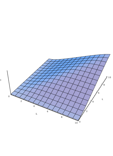
FIG. 1.: The decoherence suppression factor $D_{L}(t)$, defined as the real part of the influence phase for two trajectories in which $x$ and $x^{\prime}$ are constant in time, and differ by $L$. The environment is a massless quantum field in $n$ dimensions; the plotted function is for $n=3$ and high temperature $T\to\infty$. The $L$ and $t$ axes are in units of the UV cut-off scale $\Gamma^{-1}$, while the vertical scale is linear but arbitrary, since it depends on $g^{2}k_{B}T$.

At zero temperature ($\beta\to\infty$) it is convenient to define the functions

$$\kappa_{1}(z) = {1\over 2}[e^{z}{\rm Ei}(-z)+e^{-z}{\rm Ei}(z)]-(1+z^{2}/2)[C+\ln z]$$ (140)

$$\kappa_{3}(z) = C+\ln z-{1\over 2}[e^{z}{\rm Ei}(-z)+e^{-z}{\rm Ei}(z)]\;.$$ (141)

$C$ is Euler’s constant (often called $\gamma$ instead), and ${\rm Ei}(z)$ is the exponential-integral function[24]. In terms of these functions $\kappa_{n}$, we have

$$D_{L}(t)\big{|}_{T=0} = \kappa_{n}(\Gamma t)+\kappa_{n}(\Gamma L)-{1\over 2}\kappa_{n}\bigl{(}\Gamma(t+L)\bigr{)}$$ (143)

$$\qquad-{1\over 2}\kappa_{n}\bigl{(}\Gamma|t-L|\bigr{)},\qquad n=1,3\;.$$

For both $n=1$ and $n=3$, the behaviour of $D_{L}(t)$ is still qualitatively similar to that shown in Figure 1, even at $T=0$. The only noticeable differences are that the “ridge” along $t=L$ is sharper, especially for $n=3$, but that along the top of this ridge the function rises somewhat more gradually with increasing $t+L$.

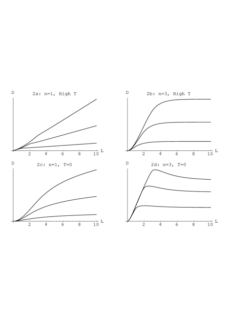
FIG. 2.: The decoherence suppression factor of Figure 1 plotted versus $L$ at three successive instants in time: $D_{L}(m\Gamma^{-1})$, for $m=1,2,3$ in order from bottom to top, i.e., successively higher curves correspond to later times. The unit of $L$ is the UV cut-off $\Gamma^{-1}$. As in Figure 1, units of $D_{L}$ are arbitrary, because each of the four functions plotted has a different prefactor involving particle-field coupling constant $g^{2}$ (whose dimensionality depends on $n$) and/or $T$. Thus all four vertical scales are linear, but they are not necessarily commensurate.

Figure 2 shows plots of $D_{L}$ versus $L$ in all four cases, at three successive instants of time $\Gamma t=1,2,3$. In each case it is clear that $D_{L}$ grows quadratically with $L$ when $L$ is small, but slows down significantly at large $L$. For $n=1$, the large $L$ behaviour is linear at high temperatures and logarithmic at zero temperature; but for $n=3$, $D_{L}$ actually approaches a constant at large $L$. In both cases, a turnover from rapid to slow growth of $D_{L}$ can be seen to occur around $L=t$ (although for $n=1$ at high temperatures this turnover becomes less and less noticeable at later times).

Even though the functions exhibited in Figures 1 and 2 are not directly related to the actual behaviour of the Brownian particle (since trajectories of constant $x$ are unlikely to dominate the path integral for any $H_{0}$), they do provide some indication of the dependence of decoherence on distance, and give a graphic illustration of the principle which is more firmly established by all the results of this Section in combination: decoherence does not grow quadratically with distance in general, but tends to saturate at large distances, in a manner that will depend in detail on the particular natures of the environment and its interaction with the system under investigation.

V Conclusion

In general, decoherence is indeed more of a minefield than a checkpoint. At low temperatures, and certainly for non-Ohmic environments, decoherence can be quite complicated even in linear systems. Noise is coloured, dissipative terms possess memory, back-reaction can have dramatic effects even on short time scales, and in general decoherence will be sensitive to all these features. With spatial non-linearity, even when noise is white and dissipation memory-less, decoherence tends to saturate at long distances, and other novel effects appear. When non-locality in time and non-linearity in space are both present, things become still more complicated, and it is clear that the simple pattern of decoherence found in Ohmic linear systems at high temperatures is drastically changed.

Since beginning work on this paper, we have become aware of the remarkable experimental work of Brune et al.[3], in which the increase of the decoherence rate as the square of the separations scale is brilliantly confirmed, albeit over a limited range of separations. Thus, there appear to be sections of the quantum-classical border which are reasonably orderly. In this paper, we are paying the current crop of experiments the highest respect of theorists: we are rushing to keep ahead of them, by considering still more complicated cases. And even so, many of the possibilities we have addressed in this paper seem likely to be encountered very soon in today’s laboratories.

A number of fascinating experiments currently under way are exploring reaches of quantum physics, such as atom optics, that have been part of quantum theory since its earliest days, and have been consistently inferred from observations, but have not hitherto been accessible to direct empirical investigation. We certainly expect these experiments to tell us much about how decoherence occurs in the real world. But almost all such experiments will be performed at low temperatures, with non-Ohmic environments and non-linear interactions. We therefore do not expect them to confirm the simple formulas that have been obtained in the first generation of theoretical studies. Rather, we hope to be able to use their results to extend our understanding of decoherence into these more complicated regimes. Experiments that have recently been proposed seem to offer yet more scope for investigating hitherto exotic aspects of decoherence. In particular, Poyatos, Cirac, and Zoller have recently shown how one can in principle produce a wide range of different interaction Hamiltonians between a harmonically trapped ion and the electromagnetic field[25]. The future of quantum decoherence as an experimental study appears to br bright; we will conclude this theoretical study with some brief comments on the experimental roles of the issues we have examined.

The experimental requirement for low temperatures in eliciting non-classical behaviour is itself evidence supporting the basic validity of the view that decoherence at high temperatures is what ensures the effective classicality of the macroscopic world. At low temperatures, however, decoherence becomes an interesting phenomenon in its own right, and not simply a robust mechanism for obtaining classical behaviour. In addition to the emergence at low temperatures of quantum kinematics, one must of course also expect the appearance of non-trivial quantum dynamics, as lower energy states predominate and the correspondence principle becomes less powerful.

Using an internal degree of freedom to enable a classical source to drive a particle into a Schrödinger’s Cat state, as in our Section III, is actually very much what is done in the remarkable recent experimental construction of a “Schrödinger’s kitten” by Monroe et al.[2]. There are also experiments that use rather the reverse approach, in which internal degrees of freedom in the environment are put into superpositions, with the result that a superposition of two different forces acts on a single system degree of freedom[13, 11]. It is no co-incidence that both of these procedures have been suggested for implementing quantum logic, since the ability to manipulate Cat-like states is the basic requirement of quantum computing. Considering decoherence that occurs during such manipulations, rather than during mere storage of a non-classical state, is therefore an important task. Our analysis in Section III is a first step in that direction. To make it more directly relevant to the various experiments will require, at the least, extending it to cases with non-Ohmic environments, in which one might expect to see non-trivial dependence of decoherence on the time-dependence of $\alpha(t)$. For example, one might expect in the case of a supra-Ohmic environment that if $\alpha(t)$ slowly grows and then shrinks again to zero, adiabatic dragging would result in decoherence that likewise rises and then diminishes dramatically. This possibility of adiabatic recoherence does not arise to any significant extent in the Ohmic regime.

The current fascinating experiments in atom optics typically involve local interactions between particles and their environments[8, 9]. One will therefore certainly expect to see the kinds of saturation effects that we have considered in Section IV. Even particles that are free, or confined in simple enough wells that the dynamics of the particles in isolation is exactly solvable, are in these cases interacting non-linearly with environmental degrees of freedom. This restricted form of non-linearity has not been extensively studied, and seems capable of providing some interesting phenomena. It is also worth noting that, in many experimental set-ups, one expects environments to be spatially inhomogeneous. (For example, in the system of Reference [10] there is an evanescent wave mirror present only at the bottom of an evacuated cavity.) This may be expected to lead to decoherence kernels that are non-trivial functions not only of off-diagonal variables like the $\Delta$ of our Section IV, but of mean spatial position as well.

There is clearly a world of experimental possibilities now opening; our message is that theory must keep up with the times. We therefore end with a theorists’ proposal for another experiment, in which decoherence should be adjustable in strength across a wide range.

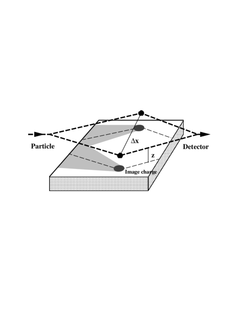
FIG. 3.: Sketch of proposed system. The heavy dashed lines indicate two trajectories of the particle over the conducting plate. The large shaded regions represent the disturbance in the electron gas inside the plate.

If charged particles are sent through a grating, interference patterns are the signature of (spatial) quantum coherence. This phenomenon is well established, and is observed consistently as long as the particle beam is isolated from environmental degrees of freedom. If an environment is deliberately introduced, however, in the form of a conducting plate over which the particles must pass before they are detected, then decoherence may occur. A calculation in classical electrodynamics [26] shows that a charge $Q$ moving at speed $v$ a constant height $z$ above a plate with resistivity $\rho$ dissipates power a rate

$$P={Q^{2}\rho v^{2}\over 16\pi z^{3}}\;.$$ (144)

This implies Ohmic damping of the particle’s motion, with a damping co-efficient proportional to $\rho z^{-3}$. Putting a layer of semi-conductor of thickness $b$ on top of the conductor multiplies (144) by $2b/3z$[27].

Since the sensitivity to $z$ is strong, and judicious choice of the conducting medium permits any $\rho$ from $10^{8}$ to $10^{-8}$ $\Omega$m, it should be possible to construct an apparatus in which the effective strength of the system-environment interaction can be varied so as to span the spectrum between the effectively classical and the purely quantum regimes. While the full quantum calculation necessary to predict the features of decoherence in this system will involve such complicated quantities as inner products between states of the conductor’s electron gas that have been disturbed by different trajectories of the particle overhead, the wide variability of the effective coupling strength should in any case allow one to walk back and forth across the quantum-classical No Man’s Land, exploring it at leisure. We are currently considering the theoretical question; we look forward to being able to compare our results with data from an experiment along these lines.

VI Acknowledgements

J.R.A. would like to thank Salman Habib for valuable discussions.

REFERENCES

- [1] W.H. Zurek, Phys. Rev. D 24, 1516 (1981); Phys. Rev. D 26, 1862 (1982).
- [2] C. Monroe, D.M. Meekhof, B.E. King, and D.J. Wineland, Science 272, 1131 (1996).
- [3] M. Brune et al., “Observing the progressive decoherence of the ‘meter’ in a quantum measurement”.
- [4] A.O. Caldeira and A.J. Leggett, Phys. Rev. A31, 1059 (1985).
- [5] W.G. Unruh and W.H. Zurek, Phys. Rev. D40, 1071 (1989).
- [6] W.H. Zurek, in G.T. Moore and M.O.Scully eds., Frontiers of Nonequilibrium Statistical Physics (Plenum: New York, 1986).
- [7] W.H. Zurek, Physics Today 44, 36 (1991).
- [8] J. Schmiedmayer et al., Phys. Rev. Lett. 74, 1043 (1995).
- [9] C.R. Ekstrom et al., Phys. Rev. A 51, 3883 (1995).
- [10] C.G. Aminoff et al., Phys. Rev. Lett. 71, 3083 (1993); related work is continuing.
- [11] P. Domokos, J.M. Raimond, M. Brune, and S. Haroche, Phys. Rev. A 52, 3554 (1995).
- [12] J. I. Cirac and P. Zoller, Phys. Rev. Lett. 74, 4091 (1995).
- [13] Q.A. Turchette, C.J. Hood, W. Lange, H. Mabuchi, and H. J. Kimble, Phys. Rev. Lett. 75, 4710 (1995).
- [14] J.R. Anglin and W.H. Zurek, Phys. Rev. D53, 7327 (1996).
- [15] B.L. Hu, J.P. Paz, and Y. Zhang, Phys. Rev. D 45, 2843 (1992).
- [16] J.P. Paz, S. Habib, and W.H. Zurek, Phys. Rev. D47, 488 (1993).
- [17] J.R. Anglin, in preparation.
- [18] J.R. Anglin, R. Laflamme, W.H. Zurek, and J.P. Paz, Phys. Rev. D 52, 2221 (1995).
- [19] Michael R. Gallis and Gordon N. Fleming, Phys. Rev. A 42, 38 (1990); 43, 5778 (1991).
- [20] N.P. Landsman and Ch. G. van Weert, Phys. Rep. 145, 141 (1987); Marcelo Gleiser and Rudnei O. Ramos, Phys. Rev. D 50, 2441 (1994).
- [21] B.L. Hu, J.P. Paz, and Y. Zhang, Phys. Rev. D 47, 1576 (1993).
- [22] M.R. Gallis, Phys. Rev. A 48, 1028 (1993).
- [23] M.R. Gallis, Phys. Rev. A 53, 655 (1996); “The emergence of classicality via decoherence: beyond the Caldeira-Leggett Environment”, quant-ph/9412002.
- [24] I.S. Gradshteyn and I.M. Ryzhik, Alan Geoffrey ed., Table of Integrals, Series, and Products, 5th ed. (Academic Press: New York, 1994), p. 993 ff. (Section 8.21).
- [25] J.F. Poyatos, J.I. Cirac, and P. Zoller, “Quantum reservoir engineering”, atom-ph/9603002.
- [26] T.H. Boyer, Phys. Rev. A 9, 68 (1974); Phys. Rev. E 53, 6450 (1996).
- [27] T.W. Darling et al., Rev. Mod. Phys. 64, 237 (1992).