Simulating Ising Spin Glasses on a Quantum Computer

Abstract

A linear-time algorithm is presented for the construction of the Gibbs distribution of configurations in the Ising model, on a quantum computer. The algorithm is designed so that each run provides one configuration with a quantum probability equal to the corresponding thermodynamic weight. The partition function is thus approximated efficiently. The algorithm neither suffers from critical slowing down, nor gets stuck in local minima. The algorithm can be applied in any dimension, to a class of spin-glass Ising models with a finite portion of frustrated plaquettes, diluted Ising models, and models with a magnetic field.

I Introduction

The algorithm of Shor [1] for the polynomial time solution of the factorization problem on a quantum computer was received with much excitement in the computer science and physics communities [2, 3]. It indicates that quantum computers have a potential for the effective solution of problems which are unfeasible on a classical computer. The actual utilization of this potential would require, in addition to many years of work on the hardware, the development of algorithms which would optimally exploit the strengths while overcoming the shortcomings of quantum computers, in particular the problem of decoherence [4, 5]. Unlike classical computers in which each bit is a two state system which can be either in state 0 or 1 the quantum bit (or qubit) can be in any superposition of the form:

$$|\psi\rangle=\alpha_{0}|0\rangle+\alpha_{1}|1\rangle,$$ (1)

as long as $|\alpha_{0}|^{2}+|\alpha_{1}|^{2}=1$. When a measurement of the qubit takes place the result will be the state $|0\rangle$ with probability $|\alpha_{0}|^{2}$ or $|1\rangle$ with probability $|\alpha_{1}|^{2}$. In the first case the system will then remain in the state $|0\rangle$ while in the second case it will remain in the state $|1\rangle$. Due to superposition, a system of $N$ qubits is described by a unit vector in a $2^{N}$ dimensional complex vector space (the Hilbert space) of the form:

$$|\psi_{N}\rangle=\sum_{i=0}^{2^{N}-1}\alpha_{i}|i\rangle,$$ (2)

where $|i\rangle$ are the $2^{N}$ basis vectors and $\sum|\alpha_{i}|^{2}=1$. Computations are done by changing the state of the system. Since conservation of probability is required only unitary transformations are allowed. One source of the potential strength of quantum computers is due to the fact that computations are performed simultaneously on all $2^{N}$ states in the superposition. This amounts to an exponential parallelism compared to classical computers in which at any given time only one number can be stored in the $N$ bit register. However, this feature alone is not enough since only a single quantum state is available after measurement [6]. The full power of quantum computation is realized only when the superposition principle is combined with the ability of quantum states to interfere. The latter has no classical analogue, and is the quantum ingredient which allows one to selectively control which state will have the highest probability of appearing after measurement.

Similarly to classical computers, it turns out that all unitary transformations involving $N$ qubits can be broken into two qubit unitary transformations [7, 8, 9, 10]. This allows one to construct a universal set of binary gates which is capable of implementing all the required operations. The actual construction of a quantum computer is a formidable task that is believed to require many years before a basic prototype will be ready. Some of the potential physical media proposed for quantum computers include ions in ion traps [11], atoms coupled to optical resonators [12], interacting electrons in quantum dots [13], and Ramsey atomic interferometry [14].

The main difficulty identified so far in the construction of a quantum computer is the decoherence of the quantum superposition due to interaction with the environment. To avoid errors one needs to isolate the quantum computer from the environment as much as possible. Some redundancy combined with error correcting codes is considered as a promising way to reduce the accumulation of errors during the computation [15, 16, 17, 18, 19, 20, 21, 22]. Another potential difficulty is to maintain sufficient precision so that the quantum computer will provide accurate results even after many steps of computing. Therefore, an efficient quantum algorithm should satisfy not only that the time and memory required for the computation grow polynomially with the input size, but also the precision: the number of bits of precision should grow only logarithmically in the input size [1, 23].

In addition to the prospects of building a quantum computer, the experimental work stimulated by this field is expected to provide new insights on the foundations of quantum mechanics, as well as to lead to progress in the development of new technologies. Furthermore, the new perspective that quantum computers provide about the complexity of algorithms is highly valuable for the theory of computation even without the physical construction of such a computer. In particular, Shor’s algorithm for the polynomial time solution of the factorization problem [1] has shown that problems which are considered intractable on classical computers may be tractable on a quantum computer, although some restrictions are known related to the potential power of a quantum computer [23]. Feynman [24] was the first to suggest that quantum computers might be exponentially faster than classical computers at simulating quantum mechanical systems with short range interactions. A general demonstration to this effect was given by Lloyd [25], who also argued that quantum computers could efficiently calculate spin-spin correlation functions in Ising models. Some explicit algorithms were later proposed for simulating physical systems on quantum computers. These include the Schrödinger equation for interacting many-body systems [26, 27, 28, 29], the Dirac equation [30] and the quantum baker’s map [31].

In this paper we consider a broad class of statistical physics problems involving Ising spin systems. We develop an algorithm for simulating these systems on a quantum computer. Here we define the Ising spin systems and briefly review the numerical techniques in use for their simulation on classical computers. These systems are important both as models of magnetic phase transitions and as the most useful models for the analytical and numerical studies of phase transitions in general [32, 33]. The numerical simulation of such systems has been an active field of research for the last five decades since the introduction of the Metropolis algorithm [34]. Typically, spin systems are defined on a $d$ dimensional lattice in which there are $N$ spins $s_{i}$, one at each lattice site $i$, and nearest neighbor coupling between spins. The energy of the system is given by the nearest-neighbor Edwards-Anderson Hamiltonian [35]:

$$H=-\sum_{\langle i,j\rangle}J_{ij}s_{i}s_{j}-\sum_{i=1}^{N}h_{i}s_{i},$$ (3)

where $\langle i,j\rangle$ represents summation only over pairs of nearest neighbors, $J_{ij}$ is the coupling between $i$ and $j$, and $h_{i}$ is the local magnetic field. The most commonly studied model is the Ising model [36] in which each spin has two states $s_{i}=\pm 1$. The bonds $J_{ij}$ then determine the nature of the interactions. In the ordinary ferromagnetic (antiferromagnetic) Ising model all bonds satisfy $J_{ij}\!=\!J$ ($J_{ij}\!=\!-J$) where $J>0$. In the $\pm J$ Ising spin glass there are quenched random bonds chosen from a bimodal distribution $P(J_{ij})\!=\!p\delta(J_{ij}-J)+(1-p)\delta(J_{ij}+J)$. The random bonds in the Ising spin glass can also be drawn from a continuous distribution such as the Gaussian distribution.

Numerical studies of spin systems have been performed for a vast variety of lattices including the square and triangular lattices in two dimensions (2D), cubic, hexagonal and hexagonal closed packed in three dimensions (3D). Here we will concentrate mainly on finite hypercubic lattices in $d$ dimensions, which include $N\!=\!L^{d}$ sites, where $L$ is the number of sites along each edge. Since each spin has two states, these Ising spin systems exhibit an exponentially large phase space of $2^{N}$ configurations. The partition function of Ising type models is given by a sum over all configurations: $Z=\sum_{\{s\}}\exp(-\beta H[\{s\}])$ where $\beta\!=\!1/(k_{B}T)$, $k_{B}$ is the Boltzmann constant and $T$ is the temperature. For a system in thermodynamic equilibrium, the partition function provides the statistical weight of each one of the $2^{N}$ configurations. The statistical weight of the configuration $\{s_{i}\},i=1,\dots,N$ is given by: ${\rm Pr}[\{s_{i}\}]\!=\!\exp(-\beta H[\{s_{i}\}])/Z$. Therefore, if the partition function is known one can obtain exact results for all the thermodynamic quantities such as the magnetization, susceptibility and specific heat. Models for which analytical calculations of this type can be performed include a variety of one dimensional (1D) models and the 2D Ising model [37]. However, for most systems of interest, including the $3D$ Ising model and most Ising spin glass models, no analytical calculation of the partition function is available [38].

The size of the input in computations of Ising spin systems is simply the number of spins $N$ plus the number of bonds $N_{B}$ which connect these spins. In models of short range interaction considered here the number of bonds is of order $O(N)$. An exact numerical calculation of the partition function or any thermodynamic quantity would involve a summation over the $2^{N}$ terms which appear in the partition function. As the system size increases the computation time would increase exponentially, and this is obviously not feasible. In order to obtain thermodynamic averages a variety of Monte Carlo methods have been developed. These methods involve a sequential random sampling of the phase space moving from one configuration to the next according to a properly designed Markov process. In order to sample all configurations with the appropriate thermodynamic weights, the Markov process must be able to access the entire phase space and to satisfy the detailed balance condition:

$${\rm Pr}(\{s_{i}\})\cdot W(\{s_{i}\}\rightarrow\{s_{i}\}^{\prime})={\rm Pr}(\{s_{i}\}^{\prime})\cdot W(\{s_{i}\}^{\prime}\rightarrow\{s_{i}\})$$ (4)

where $\{s_{i}\}$ and $\{s_{i}\}^{\prime}$ are any two states of the system and $W(\{s_{i}\}\rightarrow\{s_{i}\}^{\prime})$ is the transition probability from one state to the other in a single move of the Markov process [33]. When these conditions are satisfied one can use the Monte Carlo results to obtain approximations to thermodynamic quantities.

In the most commonly used Metropolis algorithm [34], at each time step one spin is chosen randomly. The energy difference $\Delta E$ which would occur due to flipping the chosen spin is calculated. If $\Delta E\leq 0$ the move is accepted and the spin is flipped. If $\Delta E>0$ the move is accepted with probability $p=e^{-\beta\Delta E}$. Since this rule satisfies detailed balance, one can take samples of the configurations during the run to obtain properties of the equilibrium phases such as magnetization, susceptibility, correlation function, correlation length, etc. Although for large systems it is feasible to scan only an exponentially small part of the phase space, this part typically has an exponentially large weight and therefore, Monte Carlo simulations provide good approximations for the thermodynamic quantities.

The Metropolis algorithm and related techniques which involve flipping one spin at a time are efficient as long as the system is not too close to a critical point, i.e., a second order phase transition. Near the critical point the simulation suffers from “critical slowing down” and the number of Monte Carlo steps needed between uncorrelated configurations grows as $L^{z}$ where $z$ is the dynamical critical exponent [33]. The reason for this slow dynamics is that near the critical point there are large clusters of highly correlated spins. In this situation there is a very small likelihood of flipping an entire cluster due to the large energy barrier involved. To overcome this difficulty, cluster algorithms were introduced, in which entire clusters are flipped at once, in a way that maintains detailed balance [39].

In addition to the regular lattice spin systems, there has been much interest in the study of disordered systems such as frustrated Ising models [40, 41] and the Ising spin glass [42, 43]. These systems exhibit competing ferromagnetic and antiferromagnetic interactions. In particular, in plaquettes which include an odd number of antiferromagnetic bonds it is not possible to satisfy all the bonds simultaneously and the system is thus frustrated [40, 41]. Spin glasses exhibit a complex energy landscape with a large number of metastable states or local minima. Since these minima are separated by energy barriers, when the system is simulated using Monte Carlo methods at low temperatures, it tends to be trapped around one local minimum from which it cannot escape. When the simulation is done at high temperature, the system can easily switch from the vicinity of one local minimum to another but cannot resolve the details, namely reach the local minimum itself. The approach of simulated annealing [44] in which the temperature is repeatedly raised and then slowly decreased was found useful for obtaining thermodynamic averages. In particular, it provides a probabilistic algorithm for exploring the local minima and for searching for the ground state of the system. The problem of finding the ground state of the short range 3D Ising spin glass, as well as the fully antiferromagnetic 2D Ising model in the presence of a constant magnetic field was shown by Barahona to belong to the class of non-deterministic polynomial time (NP)-hard problems, by a mapping to problems in graph theory [45, 46, 47, 48].

In this paper we present an algorithm for the study of a class of random-bond Ising spin systems on a quantum computer. By use of interference, the algorithm can construct, with linear complexity, a lattice with a fixed portion of plaquettes having predetermined bonds. The bonds connecting plaquettes are determined randomly, with the probability of obtaining a non-frustrated intermediate plaquette being higher than that of a frustrated one. The superposition property of a quantum computer can be used in order to include the entire phase space of the resulting Ising system, such that the quantum mechanical probability of each one of the $2^{N}$ states equals the thermodynamic weight of the corresponding spin configuration. In this sense the algorithm is exact. Once such a superposition is constructed one can perform a measurement of all spins, which provides one of the $2^{N}$ configurations. Since the probabilities of the quantum states are ordered by the thermodynamic weights of the corresponding spin configurations, the partition function is constructed efficiently. Putting aside questions of degeneracy, the lower the energy of the configuration, the more likely it is to be obtained upon measurement. Therefore the algorithm can be used to find ground state configurations of the spin system. Unlike Monte Carlo simulations which require a minimal number of steps between measurements to reduce the autocorrelation function between consecutively measured configurations [33], measurements on the quantum computer are totally uncorrelated since the superposition is constructed anew before every measurement. Successive runs of the algorithm therefore involve no dynamics of moving from one configuration to another. A situation in which this procedure is especially useful, is in the vicinity of a critical point, where Monte Carlo simulations may suffer from critical slowing down. While cluster algorithms have been invented for regular Ising models [39, 49] which essentially solve this problem, they are very limited in scope and can treat essentially only Ising systems with periodic bond-structure. The present algorithm is more general in that it applies to random-bond Ising models as well, and avoids the problem of critical slowing down altogether.

The paper is organized as follows. The construction of the superposition of states for the 1D Ising model, with quantum probabilities equal to the thermodynamic weights is considered in Section  II. Higher dimensional Ising systems including the Bethe lattice, the 2D and 3D Ising models are considered in Section  III. A magnetic field is introduced in Sec.IV. The conclusions appear in Section  V.

II 1D Ising Model

We begin our exposition of the algorithm by treating the simple case of a 1D Ising model. Starting from the fully ferromagnetic open chain, we will gradually introduce complexity, by considering the antiferromagnetic case, mixed ferro-antiferromagnetic models, spin-glasses, and finally close the boundary conditions. This last operation, which enables the use of transfer matrices in the classical case, allows for a comprehensive treatment of the 2D and higher dimensional models.

A The Ferromagnetic Case

The Hamiltonian for a linear, open ferromagnetic system of $N$ spins $s_{i}=\pm 1$ is [50]:

$$H^{+}_{N}=-J\sum_{i=1}^{N-1}s_{i}s_{i+1},$$ (5)

where $J>0$. Let $y\in[0,2^{N}-1]$, and $\{s\}_{y}^{N}$ be the $N$-digit binary expansion of $y$ using $s_{i}=-1$ for 0 and $s_{i}=+1$ for 1. The notation $\{s\}_{y}^{N}$ can also denote one of the $2^{N}$ spin configurations, with thermodynamic weight:

$${\rm Pr}[\{s\}_{y}]={1\over Z^{+}_{N}}e^{-\beta H^{+}_{N}[\{s\}_{y}]},$$ (6)

(the $N$ superscript on $\{s\}_{y}^{N}$ will be suppressed where it is obvious) where:

$$Z^{+}_{N}=\sum_{y=0}^{2^{N}-1}e^{-\beta H^{+}_{N}[\{s\}_{y}]},$$ (7)

is the partition function. It is the task of the algorithm to exactly calculate the probabilities above, in a manner which allows an easy identification of the configuration whose probability was found. To this end we introduce an $N$-qubit register $\{s\}_{y}^{N}=|s_{1},s_{2},...,s_{N}\rangle$, where now $s_{i}=\pm 1$ denote the ground and excited states of the $i^{\rm th}$ qubit (it is convenient to use the same notation for the classical spins and the qubits, and this should not cause any confusion). We term this a register of “spin-qubits”. Let $|\{-\}_{N}\rangle$ denote the ground state of all spin-qubits. We seek a unitary operator $T^{+}_{N}$ which simulates the Ising model in the following sense:

$$\left|\langle\{s\}_{y}^{N}|T^{+}_{N}|\{-\}_{N}\rangle\right|^{2}={\rm Pr}[\{s\}_{y}].$$ (8)

Thus $T^{+}_{N}$ evolves the qubit register into a superposition in which every state uniquely codes for an Ising configuration of spins, with a quantum probability equal to the thermodynamic weight of that configuration. $T^{+}_{N}$ must be a “valid” quantum computer operator, i.e., it must be decomposable into a product of a polynomial (in $N$) number of 1- and 2-qubit unitary operators only [4]. Such a decomposition is possible with the following two operators: a 1-qubit $\pi/2$ rotation,

$$R_{i}|s_{1},...,s_{i},...,s_{N}\rangle=$$ (10)

$${1\over\sqrt{2}}(|s_{1},...,-s_{i},...,s_{N}\rangle-s_{i}|s_{1},...,s_{i},...,s_{N}\rangle),$$

and a 2-qubit “Ising-entanglement”:

$$S^{+}_{ij}|s_{1},...,s_{i},...,s_{j},...,s_{N}\rangle=$$ (13)

$${1\over\sqrt{c}}\left(x^{-Js_{i}}|s_{1},...,s_{i},...,s_{j},...,s_{N}\rangle+\right.$$

$$\left.s_{j}x^{Js_{i}}|s_{1},...,s_{i},...,-s_{j},...,s_{N}\rangle\right),$$

where

$$x\equiv e^{\beta/2},\>\>\>\>c\equiv{1\over 2}Z^{+}_{2}=2\cosh(\beta J).$$ (14)

In what follows we will suppress the full register and indicate only the qubits operated on. It is straightforward to check that $R_{i}$ and $S^{+}_{ij}$ are indeed unitary, e.g., by considering their matrix representations in the basis where $|-\rangle=(1,0)$, $|+\rangle=(0,1)$, $|--\rangle=(1,0,0,0)$, $|-+\rangle=(0,1,0,0)$, $|+-\rangle=(0,0,1,0)$, $|++\rangle=(0,0,0,1)$:

$$R={1\over\sqrt{2}}\left(\begin{array}[]{rr}1&1\\ 1&-1\end{array}\right)$$ (17)

and

$$S^{+}={1\over\sqrt{c}}\left(\begin{array}[]{clll}x^{J}&x^{-J}&0&0\\ -x^{-J}&x^{J}&0&0\\ 0&0&x^{-J}&x^{J}\\ 0&0&\!\!\!\!\!-x^{J}&x^{-J}\\ \end{array}\right).$$ (18)

It is interesting to note the similarity to the classical 1D transfer matrix,

$$\left(\begin{array}[]{cl}x^{2J}&x^{-2J}\\ -x^{-2J}&x^{2J}\end{array}\right).$$ (19)

The $x^{J}$ vs $x^{2J}$ comes from the fact that in $S^{+}$ we have amplitudes, not probabilities.

The operator which simulates the 1D Ising problem can now be written as:

$$T^{+}_{N}=\left[\prod_{i=N-1}^{1}S^{+}_{i,i+1}\right]R_{1}.$$ (20)

Thus $T^{+}_{N}$ is a $\pi/2$ rotation of the first qubit, followed by Ising entanglements of successive pairs of qubits. This bares some resemblance to the procedure using a transfer matrix to solve the 1D Ising model. The number of required operations is exactly $N$. The general “recipe” for writing down this operator (in the absence of closed loops) is the following: one always applies a $\pi/2$ rotation to the first qubit, and then substitutes an Ising-entanglement operator for each interacting pair of nearest-neighbor spins in the Hamiltonian.

1	2	3	4	5	6
$\left|\right.s_{1},s_{2},s_{3},s_{4}\rangle$	initial	$R_{1}$	$S^{+}_{12}$	$S^{+}_{23}$	$S^{+}_{34}$
$\left|\right.----\rangle$	1	$1/\sqrt{2}$	$x^{J}/\sqrt{2c}$	$x^{2J}/\sqrt{2}c$	$x^{3J}/\sqrt{2}c^{3/2}$
$\left|\right.---+\rangle$	0	0	0	0	$-x^{J}/\sqrt{2}c^{3/2}$
$\left|\right.--+-\rangle$	0	0	0	$-1/\sqrt{2}c$	$-x^{-J}/\sqrt{2}c^{3/2}$
$\left|\right.--++\rangle$	0	0	0	0	$x^{J}/\sqrt{2}c^{3/2}$
$\left|\right.-+--\rangle$	0	0	$-x^{-J}/\sqrt{2c}$	$-x^{-2J}/\sqrt{2}c$	$-x^{-J}/\sqrt{2}c^{3/2}$
$\left|\right.-+-+\rangle$	0	0	0	0	$x^{-3J}/\sqrt{2}c^{3/2}$
$\left|\right.-++-\rangle$	0	0	0	$1/\sqrt{2}c$	$x^{-J}/\sqrt{2}c^{3/2}$
$\left|\right.-+++\rangle$	0	0	0	0	$-x^{J}/\sqrt{2}c^{3/2}$
$\left|\right.+---\rangle$	0	$1/\sqrt{2}$	$x^{-J}/\sqrt{2c}$	$1/\sqrt{2}c$	$x^{J}/\sqrt{2}c^{3/2}$
$\left|\right.+--+\rangle$	0	0	0	0	$-x^{-J}/\sqrt{2}c^{3/2}$
$\left|\right.+-+-\rangle$	0	0	0	$-x^{-2J}/\sqrt{2}c$	$-x^{-3J}/\sqrt{2}c^{3/2}$
$\left|\right.+-++\rangle$	0	0	0	0	$x^{-J}/\sqrt{2}c^{3/2}$
$\left|\right.++--\rangle$	0	0	$-x^{J}/\sqrt{2c}$	$-1/\sqrt{2}c$	$-x^{J}/\sqrt{2}c^{3/2}$
$\left|\right.++-+\rangle$	0	0	0	0	$x^{-J}/\sqrt{2}c^{3/2}$
$\left|\right.+++-\rangle$	0	0	0	$x^{2J}/\sqrt{2}c$	$x^{J}/\sqrt{2}c^{3/2}$
$\left|\right.++++\rangle$	0	0	0	0	$-x^{3J}/\sqrt{2}c^{3/2}$

TABLE I.: Amplitudes of register states for 1D Ising model with up to 4 spins.

It might be helpful to give an example at this point. For an open chain of $N\leq 4$ spins, Table I gives the amplitudes of four spins, at each stage of the algorithm, as calculated from Eq.(20). It is easily verified that the squares of the amplitudes given in columns 4, 5, 6, agree with the thermodynamic weights [given by Eq.(5)] for $N$=2, 3, 4 spins respectively, with a ferromagnetic interaction. (In order to check, e.g, for $N$=2, ignore the entries for $s_{3}$ and $s_{4}$.)

We proceed to prove that $T^{+}_{N}$ indeed satisfies Eq.(8), by mathematical induction. Let us consider first the minimal case $N=2$ (for $N=1$ we cannot apply $S^{+}$). We have $T^{+}_{2}=S^{+}_{12}R_{1}$, so that

$$T^{+}_{2}|\{-\}_{2}\rangle={1\over\sqrt{2}}S^{+}_{12}(|--\rangle+|+-\rangle)=$$ (23)

$${1\over\sqrt{2c}}\left[(x^{J}|--\rangle-x^{-J}|-+\rangle)+(x^{-J}|+-\rangle-x^{J}|++\rangle)\right]=$$

$${1\over\sqrt{2c}}\sum_{s_{1},s_{2}=\pm 1}-s_{2}x^{Js_{1}s_{2}}|s_{1},s_{2}\rangle.$$

On the other hand, according to Eq.(6) the thermodynamic weights of these four states are, respectively, $e^{\beta J}/Z^{+}_{2}$, $e^{-\beta J}/Z^{+}_{2}$, $e^{-\beta J}/Z^{+}_{2}$, $e^{\beta J}/Z^{+}_{2}$. These are exactly the squares of the above amplitudes. Next, assume by induction that Eq.(8) holds for $T^{+}_{N}$, i.e., that

$$T^{+}_{N}|\{-\}_{N}\rangle=\sum_{y=0}^{2^{N}-1}A^{+}_{y}|\{s\}_{y}\rangle,$$ (24)

where:

$$A^{+}_{y}\equiv{1\over\sqrt{Z^{+}_{N}}}x^{-H^{+}_{N}[\{s\}_{y}]}\phi_{N}$$ (26)

$$\phi_{N}\equiv-\prod_{i=2}^{N}(-s_{i}).$$

Using this, we must show that $T^{+}_{N+1}$ satisfies Eq.(8) for the 1D Ising model with $N+1$ spins. Now,

$$T^{+}_{N+1}|\{-\}_{N+1}\rangle=S^{+}_{N,N+1}T^{+}_{N}|\{-\}_{N}\rangle|-\rangle=$$ (28)

$$\sum_{y=0}^{2^{N}-1}A^{+}_{y}S^{+}_{N,N+1}|\{s\}_{y}^{N}\rangle|-\rangle,$$

where the last equality follows from the induction hypothesis. But by definition of $S^{+}$,

$$S^{+}_{N,N+1}|\{s\}_{y}^{N}\rangle|-\rangle={1\over\sqrt{c}}\left(x^{-Js_{N}}|\{s\}_{y}^{N}\rangle|-\rangle-x^{Js_{N}}|\{s\}_{y}^{N}\rangle|+\rangle\right).$$ (29)

Inserting this into Eq.(28), we have:

$$T^{+}_{N+1}|\{-\}_{N+1}\rangle=$$ (32)

$$\sum_{y=0}^{2^{N}-1}{\phi_{N}\over\sqrt{Z^{+}_{N}}}e^{-\beta H^{+}_{N}[\{s\}_{y}]/2}{1\over\sqrt{c}}\times$$

$$\left(e^{-s_{N}\beta J/2}|\{s\}_{y}^{N},-\rangle-e^{s_{N}\beta J/2}|\{s\}_{y}^{N},+\rangle\right).$$

The two terms in this sum arise from the two possible states of $|s_{N+1}\rangle$, so writing the exponents as $\exp(s_{N}s_{N+1}\beta J/2)$ and using Eq.(5), we obtain:

$$T^{+}_{N+1}|\{-\}_{N+1}\rangle=\sum_{y=0}^{2^{N+1}-1}{\phi_{N+1}\over\sqrt{Z^{+}_{N+1}}}e^{-\beta H_{N+1}[\{s\}_{y}]/2}|\{s\}_{y}^{N+1}\rangle.$$ (33)

The state $|\{s\}_{y}^{N+1}\rangle$ thus appears with a probability equal to its thermodynamic weight, which completes our proof. A useful corollary is that

Corollary 1

Upon a measurement following the execution of the algorithm, a state appears with a probability equal to the thermodynamic weight of the corresponding spin configuration.

This implies that the present algorithm provides an approximation to the partition function which converges rapidly in the number of measurements.

B The Antiferromagnetic Case

In the antiferromagnetic case, the Hamiltonian for a linear, open system of $N$ spins is

$$H^{-}_{N}=J\sum_{i=1}^{N-1}s_{i}s_{i+1},$$ (34)

where $J>0$. To treat this case we define a properly modified version of the Ising-entanglement operator $S^{+}$:

$$S^{-}_{ij}|s_{i},s_{j}\rangle={1\over\sqrt{c}}\left(x^{Js_{i}}|s_{i},s_{j}\rangle+s_{j}x^{-Js_{i}}|s_{i},-s_{j}\rangle\right).$$ (35)

In matrix form,

$$S^{-}={1\over\sqrt{c}}\left(\begin{array}[]{llcl}x^{-J}&x^{J}&0&0\\ \!\!\!\!\!-x^{J}&x^{-J}&0&0\\ 0&0&x^{J}&x^{-J}\\ 0&0&-x^{-J}&x^{J}\\ \end{array}\right)$$ (36)

and it is easily checked that $S^{-}_{ij}$ is unitary. We claim that

$$T^{-}_{N}=\left[\prod_{i=N-1}^{1}S^{-}_{i,i+1}\right]R_{1}$$ (37)

simulates the antiferromagnetic “1D Ising model”, in the sense of Eq.(8). The proof is entirely analogous to the ferromagnetic case. First one considers the case $N=2$, for which:

$$T^{-}_{2}|\{-\}_{2}\rangle={1\over\sqrt{2}}S^{-}_{12}(|--\rangle+|+-\rangle)=$$ (39)

$${1\over\sqrt{2c}}\left[(x^{-J}|--\rangle-x^{J}|-+\rangle)+(x^{J}|+-\rangle-x^{-J}|++\rangle)\right].$$

The state-probabilities are just the thermodynamic weights which can be obtained from Eq.(34) for $N=2$. Repeating the induction argument that led to Eq.(32) one finds here:

$$T^{-}_{N+1}|\{-\}_{N+1}\rangle=$$ (43)

$$\sum_{y=0}^{2^{N}-1}{\phi_{N}\over\sqrt{Z^{-}_{N}}}x^{-H^{-}_{N}[\{s\}_{y}]}\sqrt{1\over c}\times$$

$$\left(x^{s_{N}}|\{s\}_{y}^{N},-\rangle-x^{-s_{N}}|\{s\}_{y}^{N},+\rangle\right)=$$

$$\sum_{y=0}^{2^{N+1}-1}{\phi_{N+1}\over\sqrt{Z^{-}_{N+1}}}e^{-\beta H^{-}_{N+1}[\{s\}_{y}]/2}|\{s\}_{y}^{N+1}\rangle.$$

This proves that $T^{-}_{N}$ simulates the 1D antiferromagnetic Ising model.

C The “1D Spin-Glass” Case

We now consider the simplest case of a random-bond Ising model with open boundary conditions: the quenched, mixed ferro-antiferromagnetic linear chain (also known as the $\pm J$ spin glass). The Hamiltonian in this case may be written as:

$$H^{\bf J}_{N}=-\sum_{i=1}^{N-1}J_{i}s_{i}s_{i+1},$$ (44)

where ${\bf J}=(J_{1},J_{2},...,J_{N-1})$ is a fixed set of parameters, each of which can be $\pm J$ and thus determines whether the interaction between $s_{i}$ and $s_{i+1}$ is ferro- ($+$) or antiferromagnetic ($-$). There are a total of $2^{N-1}$ ${\bf J}$’s for the length-$N$ Ising chain, each of which can be regarded as a different realization of quenched disorder. The operator which simulates the corresponding Ising problem is a natural generalization of $T^{\pm}_{N}$:

$$T^{\bf J}_{N}=\left[\prod_{i=N-1}^{1}S^{J_{i}}_{i,i+1}\right]R_{1},$$ (45)

where [51]:

$$S^{J_{i}}_{ij}|s_{i},s_{j}\rangle={1\over\sqrt{c}}\left(x^{-J_{i}s_{i}}|s_{i},s_{j}\rangle+s_{j}x^{J_{i}s_{i}}|s_{i},-s_{j}\rangle\right).$$ (46)

The unitarity of $S^{J_{i}}_{ij}$ follows from the unitarity of $S^{+}_{ij}$ and $S^{-}_{ij}$. Let us prove that $T^{\bf J}_{N}$ simulates the appropriate Ising problem, again, by induction: for $N=2$ there are two realizations of the quenched disorder: $J_{1}=\pm J$. Accordingly, there are two $T^{\bf J}_{2}$’s: $T^{+}_{2}$ and $T^{-}_{2}$. We have already shown that these operators solve their corresponding Ising problem. Assume by induction that $T^{\bf J}_{N}$ simulates the Ising problem for $N$ spins. There are now four possibilities in going to $N+1$, since both $J_{N-1}$ and $J_{N}$ can be $\pm J$. In fact we have already dealt with the two cases $J_{N-1}=J_{N}$ in proving the algorithm for the fully ferro- and antiferromagnetic cases. But instead of considering separately the cases $J_{N-1}\neq J_{N}$, it will be more convenient to proceed generally. From the induction hypothesis we have:

$$T^{\bf J}_{N}|\{-\}_{N}\rangle=\sum_{y=0}^{2^{N}-1}A^{\bf J}_{y}|\{s\}_{y}^{N}\rangle\>\>;$$ (48)

$$A^{\bf J}_{y}={\phi_{N}\over\sqrt{Z^{\bf J}_{N}}}x^{-H^{\bf J}_{N}[\{s\}_{y}]}.$$

Now, $T^{\bf J}_{N+1}=S^{J_{N}}_{N,N+1}T^{\bf J}_{N}$, so that using Eq.(46):

$$T^{\bf J}_{N+1}|\{-\}_{N}\rangle|-\rangle=$$ (52)

$$\sum_{y=0}^{2^{N}-1}{\phi_{N}\over\sqrt{Z^{\bf J}_{N}}}x^{-H^{\bf J}_{N}[\{s\}_{y}]}{1\over\sqrt{c}}\times$$

$$\left(x^{-J_{N}s_{N}}|\{s\}_{y}^{N},-\rangle-x^{J_{N}s_{N}}|\{s\}_{y}^{N},+\rangle\right)=$$

$$\sum_{y=0}^{2^{N+1}-1}{\phi_{N+1}\over\sqrt{Z^{\bf J}_{N+1}}}e^{-\beta H^{\bf J}_{N+1}[\{s\}_{y}]/2}|\{s\}_{y}^{N+1}\rangle.$$

The amplitude-squared of the configuration coded by $\{s\}_{y}^{N+1}$ is exactly its thermodynamic weight for a given quenched disorder ${\bf J}$, so this completes the proof for the mixed ferro-antiferromagnetic case. Of course, the fully ferro- and antiferromagnetic cases are specific instances of this general model. The implementation of the algorithm in the present case, according to Eq.(45), would entail using (apart from the $\pi/2$ rotation), two different operators, in an order dictated by the sequence of ferro/antiferromagnetic bonds in the Ising model one wishes to solve. The complexity, however, remains $O(N)$.

The generalization to continuous interactions is straightforward. In this case:

$$H^{\bf G}_{N}=-\sum_{i=1}^{N-1}G_{i}s_{i}s_{i+1}\>,\>\>\>\>\>{\bf G}\equiv(G_{1},G_{2},...,G_{N-1}),$$ (53)

where now ${\bf G}$ is a set of independent random variables, which do not have to be identically distributed. Suppose one prepares a set ${\bf G}$. This corresponds to choosing a certain realization of quenched disorder in the Ising spin glass. The quantum operator which simulates for the thermodynamic weights in this case is

$$T^{\bf G}_{N}=\left[\prod_{i=N-1}^{1}S^{G_{i}}_{i,i+1}\right]R_{1},$$ (54)

where:

$$S^{G_{i}}_{ij}|s_{i},s_{j}\rangle=$$ (57)

$${1\over\sqrt{c_{i}}}\left(x^{-G_{i}s_{i}}|s_{i},s_{j}\rangle+s_{j}x^{G_{i}s_{i}}|s_{i},-s_{j}\rangle\right)\>;$$

$$c_{i}=2\cosh(\beta G_{i}).$$

In matrix form:

$$S^{G_{i}}={1\over\sqrt{c_{i}}}\left(\begin{array}[]{llcl}x^{G_{i}}&x^{-G_{i}}&0&0\\ \!\!\!\!\!-x^{-G_{i}}&x^{G_{i}}&0&0\\ 0&0&\>\>\>\>\>x^{-G_{i}}&x^{G_{i}}\\ 0&0&-x^{G_{i}}&x^{-G_{i}}\\ \end{array}\right)$$ (58)

The only difference from $S^{J_{i}}_{ij}$ of the $\pm J$ spin glass is that each Ising-entanglement now has its own normalization factor, which clearly has no effect on the proof of the algorithm.

As $N$ increases finite size effects diminish. By construction, our algorithm will provide in $O(N)$ steps a ground state $\{s\}^{*}$ of a “1D spin glass” with probability:

$$p^{*}=\exp(-\beta H_{N}^{\bf G}[\{s\}^{*}])/Z_{N}^{\bf G},$$ (59)

This probability can be made arbitrarily close to 1 by performing the construction for low enough temperature. If a local minimum is found instead of the ground state, the entire process should be repeated until the ground state is obtained. What is the average number of steps required for locating the global minimum in this manner? After the first run one has probability $p^{*}$ of having found $\{s\}^{*}$. If not, one failed with probability $q=1-p^{*}$ and then succeeded with probability $p^{*}$, etc. Clearly the resulting distribution is geometric, and thus the average number of runs until the global minimum is found, is $\langle n\rangle={1/p^{*}}$ [52]. The total number of steps is seen to be $O(N)/p^{*}$. The question of the complexity of the algorithm for locating a ground state thus boils down to the scaling of $p^{*}$ with $N$. In 1D this is in fact trivial: there are exactly two degenerate ground states, related by $s_{i}\rightarrow-s_{i}\>\forall i$, obtained by simply following along the chain and satisfying all bonds. Their energy is $E=-N_{B}\,J$ (where $N_{B}=N-1$ is the number of bonds) so $p^{*}=\exp(\beta N_{B}\,J)/Z_{N}$. The temperature appears here as a control parameter: let $\Delta$ be the difference in potential energy between a ground state and the next lowest states $\{s\}^{\dagger}$. Then Eq.(59) predicts that $p^{*}$ will become dominant, since $p^{*}/p^{\dagger}=\exp[\Delta/(k_{B}T)]$. This indicates that the probability of obtaining a ground state can be made arbitrarily close to 1 [53]. However, this is only true as long as the degeneracy $g_{ms}$ of metastable states with energy close (of the order of the average interaction strength $\langle G\rangle$) to the ground state energy remains small in some proper sense. For higher dimensional spin glasses, it is well known that this number is $N$-dependent. Additional complications may arise in relation to the connectivity of the system in higher dimensions. We will return to this issue in later sections. In order to be able the discuss such systems, the problem of closing the boundary conditions must first be discussed. This is done next.

D Closing the Boundary Conditions

It should be remarked that the algorithm as described so far is in fact classical. A classical probabilistic computer can run the algorithm with exactly the same efficiency simply by randomly choosing spin $s_{i}$ to be up or down with a probability determined by the thermodynamic weight of the configuration of all other $i-1$ spins and bonds. The difference is of course that the classical computer cannot store all $2^{N}$ spin configurations. However, this by itself does not enhance the computing power since only one configuration is accessible by measurement of the quantum register. The effective classicality of the algorithm is due to the fact that so far we have only employed superpositions. In Sec.II F we will employ the purely quantum effect of interference in order to deal with the problem of a 1D Ising chain with closed boundary conditions. Here we introduce the operator required for closing a 1D chain. Such a chain has as Hamiltonian in the $\pm J$ spin glass case:

$$H^{\cal J}_{N}=-\sum_{i=1}^{N}J_{i}s_{i}s_{i+1}\>;$$ (61)

$$s_{N+1}\equiv s_{1},\>\>\>\>\>{\cal J}\equiv(J_{1},J_{2},...,J_{N}).$$

A reasonable approach to closing the loop on a quantum computer might seem to be an application of the operator $S^{J_{N}}_{N,1}$ after $T^{\bf J}_{N}$. However, this does not work since it changes the amplitude of $|s_{1}\rangle$ which was already the correct thermodynamic weight. It turns out that a different approach is needed. Instead of working on $|s_{1}\rangle$, one has to first introduce a work-qubit, say $|w\rangle$, on which the Ising-entanglement operation is performed: $S^{|J_{N}|}_{N,w}$. This places $|w\rangle$ in a superposition of up and down states. Closing the loop is then performed by comparing the state of $|s_{1}\rangle$ to that of the workbit (rather than to that of $|s_{N}\rangle$), which acts effectively as the fictitious spin $s_{N+1}$. If $w=s_{1}$, the loop is closed, since this corresponds to $s_{N+1}=s_{1}$, as should be. However, one is then left to wonder what to do if $w=-s_{1}$. Instead of discarding this possibility as improper, it turns out to be fruitful to adopt a more general point of view. As will be shown in Eq.(78), the following interpretation also holds: If $w=s_{1}$, the loop is closed ferromagnetically [${\rm sign}(J_{N})=1$]; if $w=-s_{1}$, the loop is closed antiferromagnetically [${\rm sign}(J_{N})=-1$]. Since the sign of the interaction is determined randomly, we can only specify the absolute value of $J_{N}$, hence the notation $S^{|J_{N}|}_{N,w}$. The comparison operation can be performed by an exclusive-or (XOR):

$$X_{ij}|s_{i},s_{j}\rangle=s_{i}s_{j}|s_{i},s_{i}s_{j}\rangle,$$ (62)

or, in matrix form:

$$X=\left(\begin{array}[]{rrrr}0&-1&0&0\\ 1&0&0&0\\ 0&0&-1&0\\ 0&0&0&1\\ \end{array}\right)$$ (63)

Thus following $S^{|J_{N}|}_{N,w}$ one applies $X_{1,w}$; the combined operation defines a new, three-qubit operator [54]:

$$\Omega^{|J_{i}|}_{i,j,w}|s_{i},s_{j},w\rangle\equiv X_{j,w}S^{|J_{i}|}_{i,w}|s_{i},s_{j},w\rangle=$$ (66)

$$-s_{j}{1\over\sqrt{c_{i}}}\left(x^{|J_{i}|s_{i}}|s_{i},s_{j},-s_{j}w\rangle-\right.$$

$$\left.wx^{-|J_{i}|s_{i}}|s_{i},s_{j},s_{j}w\rangle\right).$$

The algorithm for simulating the closed chain “1D spin glass” can now be written as:

$$T^{\cal J}_{N}=\Omega^{|J_{N}|}_{N,1,w}T^{\rm J}_{N},$$ (67)

To prove that this formula indeed yields the correct thermodynamic weights, we may employ the result for the open-chain case, which was proved in the previous section, and include an extra state for the workbit. In the calculation to follow, a “^′” on the $\sum$ symbols indicates a sum over all spins except $s_{1}$, and:

$$\Phi_{N}=(-1)^{N}\prod_{i=1}^{N}s_{i}.$$ (68)

Now:

$$T^{\cal J}_{N}|\{-\}_{N}\rangle|w=-1\rangle=\Omega^{|J_{N}|}_{N,1,w}T^{\bf J}_{N}|\{-\}_{N}\rangle|-\rangle=$$ (71)

$$\Omega^{|J_{N}|}_{N,1,w}\sum_{y=0}^{2^{N}-1}{\phi_{N}\over\sqrt{Z^{\bf J}_{N}}}x^{-H^{\bf J}_{N}[\{s\}_{y}]}|\{s\}_{y}\rangle|w\!=\!-1\rangle=$$

$$\sqrt{2\over c_{N}}\sum_{y=0}^{2^{N}-1}{{-s_{1}\phi_{N}}\over\sqrt{Z^{\bf J}_{N}}}x^{-H^{\bf J}_{N}[\{s\}_{y}]}|\{s\}_{y}\rangle\left(x^{|J_{N}|s_{N}}|w\!=\!s_{1}\rangle+x^{-|J_{N}|s_{N}}|w\!=\!-s_{1}\rangle\right)=$$

upon collecting terms with equal $|w\rangle$:

$$\sqrt{2\over{c_{N}\,Z^{\bf J}_{N}}}\sum_{y}^{\prime}\Phi_{N}\left[\left(x^{-H^{\bf J}_{N}[\{-1,s_{2},...,s_{N}\}_{y}]}x^{-|J_{N}|s_{N}}|\{-1,s_{2},...,s_{N}\}_{y}\rangle+\right.\right.$$ (78)

$$\>\>\>\>\>\>\>\>\>\>\left.\left.x^{-H^{\bf J}_{N}[\{1,s_{2},...,s_{N}\}_{y}]}x^{|J_{N}|s_{N}}|\{1,s_{2},...,s_{N}\}_{y}\rangle\right)|+\rangle+\right.$$

$$\left.\left(x^{-H^{\bf J}_{N}[\{1,s_{2},...,s_{N}\}_{y}]}x^{-|J_{N}|s_{N}}|\{1,s_{2},...,s_{N}\}_{y}\rangle+\right.\right.$$

$$\left.\left.\>\>\>\>\>\>\>\>\>\>x^{-H^{\bf J}_{N}[\{-1,s_{2},...,s_{N}\}_{y}]}x^{|J_{N}|s_{N}}|\{-1,s_{2},...,s_{N}\}_{y}\rangle\right)|-\rangle\right]=$$

$$\sqrt{2\over{c_{N}\,Z^{\bf J}_{N}}}\sum_{y=0}^{2^{N}-1}\Phi_{N}x^{-H^{\bf J}_{N}[\{s\}_{y}]}|\{s\}_{y}\rangle\left(x^{s_{N}s_{1}|J_{N}|}|+\rangle+x^{-s_{N}s_{1}|J_{N}|}|-\rangle\right)=$$

$$\sqrt{2\over{c_{N}\,Z^{\bf J}_{N}}}\sum_{{\rm sign}(J_{N})}\sum_{y=0}^{2^{N}-1}\Phi_{N}x^{-H^{\bf J}_{N}[\{s\}_{y}]}x^{J_{N}s_{N}s_{1}}|\{s\}_{y}\rangle|{\rm sign}(J_{N})\rangle=$$

$$\sum_{{\rm sign}(J_{N})}\sum_{y=0}^{2^{N}-1}{\Phi_{N}\over\sqrt{Z^{\cal J}_{N}}}e^{-\beta H^{\cal J}_{N}[\{s\}_{y}]/2}|\{s\}_{y}\rangle|{\rm sign}(J_{N})\rangle.$$

Since the amplitude-squared of the state $|\{s\}_{y}\rangle$ is given by the thermodynamic weight of the corresponding 1D, closed-chain spin glass system, we have proved that the algorithm which includes a workbit works for closed boundary conditions.

How should one interpret the “$|{\rm sign}(J_{N})\rangle$” in the last line of Eq.(78)? The workbit is in the excited- or ground state according to whether ${\rm sign}(J_{N})$ is positive or negative, respectively. That is, the state of the workbit is determined by whether the interaction between spins $s_{1}$ and $s_{N}$ is ferro- or antiferromagnetic. However, in the simulation of Ising models one is interested in a specific set of bonds, so it is necessary to be able to determine the last bond-sign. This is especially important for higher dimensional models, where every plaquette corresponds to a closed 1D chain. For this reason we will next present a detailed analysis of the complexity associated with generating a single plaquette. Before doing so, we note that a useful corollary follows from the calculation above, given that there was no special importance to the indices of the spins between which the loop was closed:

Corollary 2

Closing the bond between $s_{i}$ and $s_{j}$ using $\Omega^{|J|}_{ijw}$ always produces a superposition with half the states having probabilities equal to the thermodynamic weight of the Hamiltonian with a ferromagnetic $J_{ij}$, and the other half with antiferromagnetic $J_{ij}$.

Now, the simplest way of determining the last bond sign is to measure it, following the application of $\Omega^{|J_{N}|}_{N,1,w}$. This irreversible, nonunitary operation collapses the superposition of $|w\rangle$ while leaving the superposed state of the spin-qubits intact. It randomly chooses between a ferro- or antiferromagnetic bond connecting $s_{1}$ and $s_{N}$, i.e., chooses between ${\rm sign}(J_{N})=\pm 1$. Measurements are tantamount to classical operations, so in light of the comment at the beginning of this section, a measurement as a means of choosing the last bond sign leaves the algorithm in the classical realm. Therefore it may not come as a surprise that measurements will prove to be ineffective as a means of obtaining the desired last bond sign. Instead, one may employ interference in order to “erase” one of the last bonds, and leave only the desired one. In the following two sections we will discuss both procedures in detail.

E Measurements as a Means of Choosing the Desired Bond Sign

A measurement of the workbit collapses its superposition into either the ferro- or antiferromagnetic state. As we now show, which last bond sign has the higher probability depends on whether the resulting closed chain is frustrated or not. From the result of Eq.(78) we have for the $\pm J$ spin glass:

$$\Omega^{|J_{N}|}_{N,1,w}T^{\bf J}_{N}|\{-\}_{N}\rangle|-\rangle=$$ (80)

$$\sum_{{\rm sign}(J_{N})=\pm 1}\sum_{y=0}^{2^{N}-1}{\Phi_{N}\over\sqrt{Z^{\cal J}_{N}}}e^{-\beta H^{\cal J}_{N}[\{s\}_{y}]/2}|\{s\}_{y}\rangle|{\rm sign}(J_{N})\rangle,$$

where ${\cal J}\equiv(J_{1},J_{2},...,J_{N})$ and $|J_{i}|=J$. Let us now define the “partial partition functions” $Z_{N}^{J_{N}}$, i.e., $Z_{N}^{+}$ for a ferromagnetic bond between $s_{1}$ and $s_{N}$, and $Z_{N}^{-}$ for an antiferromagnetic bond. The relative weight of the ferro- and antiferromagnetic subspaces can then be expressed as: $r=Z_{N}^{+}/Z_{N}^{-}$. Without loss of generality, let us assume from now on that an antiferromagnetic last bond results in a frustrated system (i.e., the total number of antiferromagnetic bonds is odd), and vice versa. Then $r$ determines the relative probability of obtaining a frustrated or unfrustrated chain as a result of the measurement on the workbit. It is intuitively clear that the spin configurations of a frustrated system will generally have a higher energy than those of the corresponding unfrustrated system, and one would thus expect to find $Z_{N}^{+}>Z_{N}^{-}$. In 1D this statement can be made exact, as we now show. Separating the last bond one finds:

$$Z_{N}^{J_{N}}=\sum_{y=0}^{2^{N}-1}e^{-\beta\left(H^{\rm J}_{N}[\{s\}_{y}]-J_{N}s_{N}s_{1}\right)},$$ (81)

which can be split into two terms, corresponding to $s_{1}=s_{N}$ and $s_{1}=-s_{N}$:

$$Z_{N}^{J_{N}} = \left[\sum_{{\{s\}}_{N}}^{\prime}e^{-\beta\left(H^{\rm J}_{N}\left[\{s\}_{s_{1}=s_{N}}\right]-J_{N}\right)}\right.$$ (82)

$$+ \left.\sum_{{\{s\}}_{N}}^{\prime}e^{-\beta\left(H^{\rm J}_{N}\left[\{s\}_{s_{1}=-s_{N}}\right]+J_{N}\right)}\right].$$ (83)

Defining $H_{N}^{0}[\{s\}]\equiv H^{\rm J}_{N}\left[\{s\}_{s_{1}=s_{N}}\right]$ and $H_{N}^{1}[\{s\}]\equiv H^{\rm J}_{N}\left[\{s\}_{s_{1}=-s_{N}}\right]$, we can write this as:

$$Z_{N}^{J_{N}}=\left(x^{2J_{N}}Z_{N}^{0}+x^{-2J_{N}}Z_{N}^{1}\right),$$ (85)

$$Z_{N}^{0,1}\equiv\sum_{\{s\}}^{\prime}e^{-\beta H_{N}^{0,1}[\{s\}]}.$$

Using this:

$${Z_{N}^{+}\over Z_{N}^{-}}={{x^{2J}Z_{N}^{0}+x^{-2J}Z_{N}^{1}}\over{x^{-2J}Z_{N}^{0}+x^{2J}Z_{N}^{1}}}.$$ (86)

The “constrained” Hamiltonians, where $s_{N}=\pm s_{1}$ can be written as:

$$H_{N}^{0} = -\sum_{i=1}^{N-2}J_{i}s_{i}s_{i+1}-J_{N-1}s_{N-1}s_{N}$$ (87)

$$= H_{N-1}^{\bf J}-J_{N-1}s_{N-1}s_{1}$$ (88)

$$H_{N}^{1} = H_{N-1}^{\bf J}+J_{N-1}s_{N-1}s_{1}.$$ (89)

This allows one to break up the constrained partition functions in a manner similar to Eq.(83):

$$Z_{N}^{0} = \sum_{\{s\}}e^{-\beta\left(H^{\rm J}_{N-1}[\{s\}]-J_{N-1}s_{N-1}s_{1}\right)}$$ (90)

$$= \left[\sum_{\{s\}}^{\prime}e^{-\beta\left(H^{\rm J}_{N-1}\left[\{s\}_{s_{1}=s_{N-1}}\right]-J_{N-1}\right)}\right.$$ (91)

$$+ \left.\sum_{\{s\}}^{\prime}e^{-\beta\left(H^{\rm J}_{N-1}\left[\{s\}_{s_{1}=-s_{N-1}}\right]+J_{N-1}\right)}\right]$$ (92)

$$= \left(x^{2J_{N-1}}Z_{N-1}^{0}+x^{-2J_{N-1}}Z_{N-1}^{1}\right).$$ (93)

Similarly,

$$Z_{N}^{1}=\left(x^{-2J_{N-1}}Z_{N-1}^{0}+x^{2J_{N-1}}Z_{N-1}^{1}\right).$$ (94)

One may continue to split up the Hamiltonians as in Eq.(89). The general pattern is seen to be ($0\leq n\leq N-3$):

$$Z_{N-n}^{0}=2\left(x^{2J_{N-n-1}}Z_{N-n-1}^{0}+x^{-2J_{N-n-1}}Z_{N-n-1}^{1}\right)$$ (95)

$$Z_{N-n}^{1}=2\left(x^{-2J_{N-n-1}}Z_{N-n-1}^{0}+x^{2J_{N-n-1}}Z_{N-n-1}^{1}\right).$$ (96)

Together with the obvious initial condition for a pair of spins, $Z_{2}^{0}=2x^{2J_{1}}$, $Z_{2}^{1}=2x^{-2J_{1}}$, this defines a recursion relation which can be solved to yield for Eq.(85) ($N\geq 3$):

$$Z_{N}^{J_{N}}={2^{N-2}\over x^{2\left(J+\sum_{i=1}^{N-1}J_{i}\right)}}\sum_{k=0}^{N-1}x^{2(J+(-1)^{k+N-1}J_{N})}f_{N}(k).$$ (97)

where:

$$f_{N}(k)=\sum_{i_{1}<i_{2}<...<i_{k}=k}^{N-1}x^{4\sum_{j=1}^{k}J_{i_{j}}}\>\>\>\>;\>\>f_{N}(0)=1.$$ (98)

The last function generates all possible different sums of the $J_{i}$’s. For example, for $N=4$ we find:

$${Z_{4}^{+}\over Z_{4}^{-}}={{{[1]+x^{4J}\left[x^{4J_{1}}+x^{4J_{2}}+x^{4J_{3}}\right]+\left[x^{4(J_{1}+J_{2})}+x^{4(J_{1}+J_{3})}+x^{4(J_{2}+J_{3})}\right]+x^{4J}\left[x^{4(J_{1}+J_{2}+J_{3})}\right]}}\over{\left[x^{4J}\right]+\left[x^{4J_{1}}+x^{4J_{2}}+x^{4J_{3}}\right]+x^{4J}\left[x^{4(J_{1}+J_{2})}+x^{4(J_{1}+J_{3})}+x^{4(J_{2}+J_{3})}\right]+\left[x^{4(J_{1}+J_{2}+J_{3})}\right]}}.$$ (99)

It can be checked that this agrees with the result obtained directly from the corresponding Hamiltonians, and indeed, Eq.(97) can be proved to hold by induction [55]. The important point about Eq.(97) is the difference between $Z_{N}^{+}$ and $Z_{N}^{-}$. As can be seen in Eq.(99), there is an alternating ratio of $x^{4J}$ between groups of similar terms in $Z_{N}^{+}$ and $Z_{N}^{-}$. “Similar terms” here refers to terms with the same number of $J_{i}$’s, enclosed in brackets in Eq.(99). Since there is a one-to-one correspondence of this type, we may utilize the elementary inequality [56]

$$\min_{i}\left({a_{i}\over b_{i}}\right)\leq{\sum_{i}^{N}a_{i}\over\sum_{i}^{N}b_{i}}\leq\max_{i}\left({a_{i}\over b_{i}}\right),$$ (100)

to obtain that:

$$\min\left(x^{4J},x^{-4J}\right) = x^{-4|J|}$$ (101)

$$\leq {Z_{N}^{+}\over Z_{N}^{-}}\leq x^{4|J|}=\max\left(x^{4J},x^{-4J}\right).$$ (102)

The upper bound is approached as $T\!\rightarrow\!0$. To see this, use Eq.(97) to express the ratio of unfrustrated to frustrated partition functions as:

$${Z_{N}^{+}\over Z_{N}^{-}}={{\sum_{k=0}^{N-1}x^{2J(1-(-1)^{k+N})}f_{N}(k)}\over{\sum_{k=0}^{N-1}x^{2J(1+(-1)^{k+N})}f_{N}(k)}},$$ (103)

Since $J_{N}\!<\!0$ results in a frustrated system, when $N$ is odd there must be an even number $k_{e}^{*}$ (zero included) of ferro- and even number of antiferromagnetic bonds among the first $N\!-\!1$ $J_{i}$’s. When $N$ is even, there must be an odd number $k_{o}^{*}$ of ferro- and even number of antiferromagnetic bonds among the first $N\!-\!1$ $J_{i}$’s. Now, as $T\!\rightarrow\!0$ the dominant term in both numerator and denominator of Eq.(103) will be the one which has all the positive $J_{i}$’s (such a term exists, since $f_{N}(k)$ generates all combinations of $J_{i}$’s). When $T$ is sufficiently low, all other terms become negligible, since they are smaller by at least $x^{4J}$. Thus to understand the low $T$ behavior of Eq.(97) it suffices to consider that of the dominant terms. As can be seen from the expression for $f_{N}(k)$, $k$ counts how many $J_{i}$’s appear in every term. Thus for odd $N$ the dominant term is generated when $k\!=\!k_{e}^{*}$ (is even), whereas for even $N$, the dominant term results when $k\!=\!k_{o}^{*}$ (is odd). In both cases $k\!+\!N$ is odd. But this means that $2(J\!-\!(-1)^{k+N}J_{N})$ is zero in the frustrated ($J_{N}\!=\!-J$) case, $4J$ in the unfrustrated case. Thus the dominant term in the unfrustrated case is always greater by $x^{4J}$ than that of the frustrated case. This proves that the upper bound in Eq.(102) is indeed reached as $T\!\rightarrow\!0$. The implication is that an algorithm which attempts to generate frustrated isolated plaquettes by measurement alone, will have to try an average of $\sim\!x^{4J}$ times before succeeding, and this number grows exponentially as the temperature is lowered.

One might be tempted to try to correct a “wrong” plaquette instead of “discarding” it. However, it turns out that any correction procedure has probability less than 1 of succeeding. For example, suppose one is interested in the frustrated case, but the measurement yielded an unfrustrated plaquette. The problem is then that $H^{\cal J}_{N}$ includes the bond $J_{N}$ with the wrong sign. One could imagine several strategies to “undo” this, which all start with a new workbit $w^{\prime}$. For example, one could employ a “biased random walk” procedure: one redoes $\Omega^{|J_{N}|}_{N,1,w^{\prime}}$, measures again, etc. The hope is that the resulting sum of $J_{N}$’s with random signs will at one point add up to produce the originally desired ferromagnetic bond. The probability for this to happen is equal to the probability of return of some biased random walk where the bias increases with the distance from the origin. For the unbiased random walker in 1D and 2D this probability is 1, but the waiting time is infinite [57]. For the biased random walker the probability of return turns out to be zero. This means that a “random walker” correction procedure cannot guarantee the desired result, at constant temperature. We are not aware of any other, more successful procedure. What about turning a frustrated last bond into an unfrustrated one? Even this has probability less than 1, as a consideration of a three-spin system will illustrate: Suppose one chooses $J_{1}\!=\!J_{2}\!=\!J$ and after measuring $w$ one finds $J_{3}\!=\!-J$. One might then hope to correct this frustrated system by redoing $\Omega^{|J_{3}|}_{3,1,w^{\prime}}$. A low $T$ analysis will suffice to show that this will not correct the error. At low $T$ the dominant spin configuration will be that with the lowest energy $E_{min}$. It is easily checked that both $w^{\prime}=\pm 1$ yield $E_{min}\!=\!-2J$ and thus have equal probability. The case $w^{\prime}=1$ corresponds to a ferromagnetic last bond and therefore corrects the Hamiltonian. However, in the equally probable opposite case the Hamiltonian now includes a last bond of strength $J_{3}\!=\!-2J$. If this had been the result of the correction procedure, one would be facing a (wrongly) biased random walk again, since a new measurement would either result in $J_{3}\!=\!J$ or $J_{3}\!=\!-3J$, with corresponding $E_{min}\!=\!-J$ and $E_{min}\!=\!-3J$. The latter is more probable by a factor $e^{2\beta J}$, so the correction fails.

These arguments show that procedures using only combinations of superposition and measurement, have no control over the type of plaquette they generate. In the next section we will introduce a procedure which does have this feature.

F Using Interference to Close an Isolated Plaquette

After closing the last bond, the quantum register is in a superposition corresponding to a frustrated ($w=-1$) and unfrustrated ($w=1$) plaquette [Eq.(78)] (assuming, without loss of generality, that there is an even number of antiferromagnetic bonds among the first $N-1$ bonds):

$$|\psi\rangle=T^{\cal J}_{N}|\{-\}_{N}\rangle|w=-1\rangle=|\psi_{-}\rangle+|\psi_{+}\rangle,$$ (104)

where

$$|\psi_{\pm}\rangle={1\over\sqrt{Z^{\cal J}_{N}}}\sum_{y=0}^{2^{N}-1}\Phi_{N}x^{-H_{\pm}[\{s\}_{y}]}|\pm\rangle|\{s\}_{y}\rangle,$$ (105)

and where $H_{\pm}$ corresponds to $J_{N}=\pm J$. We have intentionally written the workbit first, so that in the binary representation of the spin configurations by the quantum register, the first $2^{N}$ states correspond to the frustrated configurations ($w\!=\!-1$) and the last $2^{N}$ correspond to the unfrustrated configurations ($w\!=\!+1$). As was shown in the previous section, achieving control over the plaquette type cannot be done by measurement alone. However, one may try to employ interference in order to “erase” one of the subspaces, thus leaving only the desired plaquette type. To see this, consider the wavefunction $|\psi\rangle$ of the quantum register as a vector of length $2^{(N+1)}$, with the first $2^{N}$ entries corresponding to $|\psi_{-}\rangle$, and the last $2^{N}$ entries corresponding to $|\psi_{+}\rangle$. Within each such subspace, the entries run over all possible spin configurations $y=0...2^{N}-1$. Clearly $\langle\psi|\psi\rangle\!=\!1$ by unitarity of $T^{\cal J}_{N}$. We now seek a new unitary transformation $U$ such that:

$$U_{\pm}|\psi\rangle={1\over\sqrt{Z_{\pm}}}|\psi_{\pm}\rangle\>\>\>\>\>;\>\>Z_{\pm}=\langle\psi_{\pm}|\psi_{\pm}\rangle.$$ (106)

Thus $U$ rotates the superposed quantum register state $|\psi\rangle$ into a state representing either the frustrated or the unfrustrated configurations. That $U$ exists is clear since it takes one norm 1 vector into another. Furthermore it clearly mixes different spin configurations, i.e., creates interferences. The problem is to find $U$, given that it is a $2^{(N+1)}\cdot 2^{(N+1)}$ matrix of coefficients that depend on $\cal J$. In other words, one needs to know the Gibbs distribution of the plaquette as input in order to find $U$! This might seem to defeat the purpose of the algorithm altogether, but not so in view of the need to construct plaquettes with given bonds for the 2D and 3D Ising problems. In these higher dimensional cases it is very useful to know how to produce small plaquettes of, e.g., 3 or 4 spins, for the triangular and square lattices respectively. Thus in these cases, or indeed for any plaquette of $N$ spins, one could calculate in advance the Gibbs distribution, find $U$, and use it in the construction of a lattice. We will deal with the question of “integration” of a plaquette into a lattice in Sec.III B. Here we give the general (classical) algorithm for the construction of $U$ for any $N$, and explicitly solve the cases $N=3,4$.

1 General Construction of $N$-Spin Interference Operator

Let $\{\hat{e}_{i}\}_{i=1}^{2n}$, $n=2^{N}$, be the standard basis of vectors for ${\cal R}^{2n}$, with a 1 at position $i$, zeroes elsewhere. Consider a normalized real vector ${\bf v}$ of length $2n$ (representing $|\psi\rangle$) and another vector ${\bf w}$ composed of ${\bf v}$’s upper half, also normalized: ${\bf w}=(v_{1},v_{2},...,v_{n},0,0,...,0)/\alpha_{-}$ where $\alpha_{-}=\left(\sum_{i=1}^{n}v_{i}^{2}\right)^{1/2}$. Here ${\bf w}$ corresponds to $|\psi_{-}\rangle$. We seek a construction by two-qubit operations of a unitary matrix $U_{\_}$ such that $U_{\_}{\bf v}={\bf w}$ [as in Eq.(106)]. The solution to this problem is within the theory of generators of $SO(n)$, as outlined in Ref.[58], in terms of generalized Euler angles. Since in our case ${\bf v}$ and ${\bf w}$ are real vectors, it suffices to find an orthogonal $U_{\_}$. The idea is to first rotate ${\bf w}$ so that it coincides with $\hat{e}_{n}$, and then solve the easier problem of finding the transformed $U_{\_}$ which rotates the transformed ${\bf v}$ into $\hat{e}_{n}$. More explicitly, suppose one has found an orthogonal matrix $G_{-}^{(1)}$ satisfying: ${\bf w}\!=\!G_{-}^{(1)}\hat{e}_{n}$. Clearly $G_{-}^{(1)}$ is composed of two blocks, an upper block $G_{-}^{\prime(1)}$ and a lower one $I_{n}$, the $n\!\cdot\!n$ identity matrix. The transformed equation is then: $G_{-}^{(2)}{\bf v}^{\prime}=\hat{e}_{n}$, with $G_{-}^{(2)}\!=\!(G_{-}^{(1)})^{-1}U_{\_}G_{-}^{(1)}$ and:

$${\bf v}^{\prime} = (G_{-}^{(1)})^{-1}{\bf v}=(G_{-}^{(1)})^{-1}(\alpha_{-}{\bf w}+\sum_{i=n+1}^{2n}v_{i}\hat{e}_{i})$$ (107)

$$= (\overbrace{0,0,..,\alpha_{-}}^{n},v_{n+1},...,v_{2n}).$$ (108)

Since only the last $n\!+\!1$ coordinates of ${\bf v}^{\prime}$ are non-zero, $G_{-}^{(2)}$ is composed of an upper block $I_{n-1}$ and a lower block $G_{-}^{\prime(2)}$ which we need to find along with $G_{-}^{\prime(1)}$. Having found these, the solution can be written as:

$$U_{\_}\!=\!G_{-}^{(1)}G_{-}^{(2)}(G_{-}^{(1)})^{-1}.$$ (109)

Following Ref.[58], let us write:

$$G_{-}^{(1)}=\prod_{i=1}^{n-1}g_{i}(\theta_{i}),\>\>\>\>G_{-}^{(2)}=\prod_{i=n}^{2n-1}g_{i}(\theta_{i}),$$ (110)

where $g_{i}(\theta_{i})$, is a rotation by $\theta_{i}$ in the plane spanned by $(\hat{e}_{i},\hat{e}_{i+1})$ of ${\cal R}^{2n}$:

$$g_{i}(\theta_{i})=\left(\begin{array}[]{crcc}I_{i-1}&&&\\ &\cos\theta_{i}&\sin\theta_{i}&\\ &-\sin\theta_{i}&\cos\theta_{i}&\\ &&&I_{2n-i-1}\\ \end{array}\right),$$ (111)

Application of $G_{-}^{(1)}$ to $\hat{e}_{n}$ results in the following set of equations:

$$w_{n}=\cos\theta_{n-1}$$ (117)

$$w_{n-1}=\sin\theta_{n-1}\cos\theta_{n-2}$$

$$w_{n-2}=\sin\theta_{n-1}\sin\theta_{n-2}\cos\theta_{n-3}$$

$$\cdots$$

$$w_{2}=\sin\theta_{n-1}\sin\theta_{n-2}\cdots\sin\theta_{2}\cos\theta_{1}$$

$$w_{1}=\sin\theta_{n-1}\sin\theta_{n-2}\cdots\sin\theta_{2}\sin\theta_{1},$$

with solution ($k=1,...,n-1$):

$$\cos\theta_{k}={v_{k+1}\over{r_{k+1}}}$$ (120)

$$\sin\theta_{k}={r_{k}\over{r_{k+1}}}$$

$$r_{j}=\left(\sum_{i=1}^{j}v_{i}^{2}\right)^{1/2}$$

Similarly, application of $(G_{-}^{(2)})^{-1}$ to $\hat{e}_{n}$ results in:

$$v^{\prime}_{n}=\cos\theta_{n}$$ (126)

$$v^{\prime}_{n+1}=\sin\theta_{n}\cos\theta_{n+1}$$

$$v^{\prime}_{n+2}=\sin\theta_{n}\sin\theta_{n+1}\cos\theta_{n+2}$$

$$\cdots$$

$$v^{\prime}_{2n-1}=\sin\theta_{n}\sin\theta_{n+1}\cdots\sin\theta_{2n-2}\cos\theta_{2n-1}$$

$$v^{\prime}_{2n}=\sin\theta_{n}\sin\theta_{n+1}\cdots\sin\theta_{2n-2}\sin\theta_{2n-1},$$

yielding ($k=n,...,2n-1$):

$$\cos\theta_{k}={v^{\prime}_{k}\over r_{k}}$$ (129)

$$\sin\theta_{k}={r_{k+1}\over r_{k}}\>,\>\>\>\sin\theta_{2n-1}=-{r_{k+1}\over r_{k}}$$

$$r_{j}=\left(\sum_{i=j}^{2n}v_{i}^{\prime 2}\right)^{1/2}.$$

The case ${\bf w}\!=\!(0,...,0,v_{n+1},...,v_{2n})/\alpha_{+}$, with $\alpha_{+}=\left(\sum_{i=1}^{n}v_{i}^{2}\right)^{1/2}$, corresponds to $|\psi_{+}\rangle$, and we need to find an orthogonal $U_{+}$ such that $U_{+}{\bf v}\!=\!{\bf w}$. It can be seen by repeating the arguments above that we now require ${\bf w}\!=\!G_{+}^{(1)}\hat{e}_{n+1}$, whence $G_{+}^{(1)}$ has $I_{n}$ as its upper block, and ${\bf v}^{\prime}\!=\!G_{+}^{(1)}{\bf v}\!=\!(v_{1},...v_{n},\alpha_{+},0,...,0)$ satisfies the transformed equation ${\bf v}^{\prime}\!=\!G_{+}^{(2)}\hat{e}_{n+1}$, where $G_{+}^{(2)}\!=\!G_{+}^{(1)}U_{+}^{-1}(G_{+}^{(1)})^{-1}$ has $I_{n-1}$ as its lower block. Writing accordingly

$$G_{+}^{(1)}=\prod_{i=n+1}^{2n-1}g_{i}(\theta_{i}),\>\>\>\>G_{+}^{(2)}=\prod_{i=1}^{n}g_{i}(\theta_{i}),$$ (130)

leads to equations very similar to Eqs.(117-129): one needs to replace $w_{i}$ and $v_{i}$ by $v^{\prime}_{i}$ everywhere in Eqs.(117-120), as well as allow $k$ to range from 1 to $n$. In Eq.(126) one should replace $v^{\prime}_{i}$ by $w_{i}$, whereas in Eq.(129) $k$ should range from $n+1$ to $2n-1$ and $v^{\prime}_{i}$ replaced by $v_{i}$. With these replacements it follows that the $\theta_{i}$ are identical for $U_{-}$ and $U_{+}$, except for $\theta_{n}$, for which $\sin\theta_{n}^{+}\!=\!\cos\theta_{n}^{-}$. The interference matrix is given by:

$$U_{+}\!=\!(G_{+}^{(1)})^{-1}G_{+}^{(2)}G_{+}^{(1)}.$$ (131)

This, together with Eqs.(108),(109), uniquely solves our problem. It remains to be shown explicitly how $U_{\pm}$ can be written in terms of one and two-qubit operations on the original spin-qubit register.

We note that the $g_{i}(\theta_{i})$ are identity matrices except for $2\!\cdot\!2$ blocks. Consider the representation of the basis $\{\hat{e}_{i}\}$ by ${\bf s}^{\prime}\!=\!\{|s^{\prime}_{1},...,s^{\prime}_{N}\rangle\}_{y^{\prime}=0}^{2^{N}-1}$ where the successive register states differ by a single qubit flip. In this basis application of each $g_{i}(\theta_{i})$ does not entangle states differing by more than one qubit, so the corresponding $\hat{g}_{i}(\theta_{i})$ is a single-qubit operator:

$$\hat{g}_{i}(\theta_{i})|s_{i}\!=\!-1\rangle=\cos\theta_{i}|-\rangle+\sin\theta_{i}|+\rangle$$ (133)

$$\hat{g}_{i}(\theta_{i})|s_{i}\!=\!+1\rangle=-\sin\theta_{i}|-\rangle+\cos\theta_{i}|+\rangle.$$

The remaining problem is thus seen to be the transformation from the original “binary” basis $\{|s_{1},...,s_{N}\rangle\}_{y=0}^{2^{N}-1}$ to ${\bf s}^{\prime}$ and back. This is easily accomplished by two-qubit operations using the well-known classical Gray code [59]. The Gray-to-binary transformation is accomplished by successive XORs starting from the last qubit [these differ somewhat from the definition in Eq.(62), hence the different notation]:

$$X^{\prime}_{i,j}|s_{i},s_{j}\rangle\rightarrow|s^{\prime}_{i},s^{\prime}_{j}\rangle=|s_{i},-s_{i}s_{j}\rangle,$$ (134)

where an extra workbit $w_{x}$ represent $s_{0}\equiv-1$. For example, for the two successive binary ${\bf s}$ basis states $|w_{x},s_{1},s_{2},s_{3},s_{4}\rangle\!=\!|-,-,+,+,+\rangle$ and $|-,+,-,-,-\rangle$ we find after application of $\prod_{i=0}^{3}X^{\prime}_{i,i+1}$: $|-,-,+,-,-\rangle$ and $|-,+,+,-,-\rangle$ respectively, which indeed differ by only a single qubit. Furthermore, clearly $X^{\prime-1}_{i,j}\!=\!X^{\prime}_{i,j}$ so the binary-to-Gray transformation is accomplished by running the same sequence of XORs in reverse order (starting from the extra workbit). We can now finally write down the full interference transformation. Let:

$$X^{\prime}_{N}\equiv X^{\prime}_{w_{x},w}X^{\prime}_{w,1}\prod_{i=1}^{N-1}X^{\prime}_{i,i+1},$$ (135)

and:

$$\hat{G}_{-}^{(1)}=\prod_{i=1}^{2^{N}-1}\hat{g}_{i}(\theta_{i})\>\>\>\>\>\>\>\hat{G}_{-}^{(2)}=\prod_{i=2^{N}}^{2^{N+1}-1}\hat{g}_{i}(\theta_{i})$$ (137)

$$\hat{G}_{+}^{(1)}=\prod_{i=2^{N}+1}^{2^{N+1}-1}\hat{g}_{i}(\theta_{i})\>\>\>\hat{G}_{+}^{(2)}=\prod_{i=1}^{2^{N}}\hat{g}_{i}(\theta_{i}).$$

The inverse operators are obtained by reversing the order of the products and negating all angles. Then:

$$|w_{x}\rangle|\psi_{-}\rangle=X^{\prime-1}_{N}{\hat{G}_{-}}^{(1)}{\hat{G}_{-}}^{(2)}({\hat{G}_{-}}^{(1)})^{-1}X^{\prime}_{N}|w_{x}\rangle|\psi\rangle$$ (139)

$$|w_{x}\rangle|\psi_{+}\rangle=X^{\prime-1}_{N}({\hat{G}_{+}}^{(1)})^{-1}({\hat{G}_{+}}^{(2)})^{-1}{\hat{G}_{+}}^{(1)}X^{\prime}_{N}|w_{x}\rangle|\psi\rangle$$

expresses the interference transformation leaving only the register states corresponding to frustrated or unfrustrated spin configurations.

2 Solution for $N=3,4$ Spin System

We now employ the above formalism in order to explicitly solve for the interference transformations of the three- and four-spin systems, corresponding to the elementary cells of the triangular and square lattices respectively. First it should be noted that for the $\pm J$ model in 1D, for a closed Ising chain of given length, the spectra of all frustrated realizations of bond choices are identical, and so are the spectra of all unfrustrated realizations. To see this, consider a specific spin configuration and realization of bonds with energy $E$, and suppose one changes the sign of some arbitrary pair of bonds $J_{m},J_{n}$, $m<n$. This operation does not change the frustration of the chain, since this is determined by the parity of antiferromagnetic bonds. But by flipping all spins $s_{m+1},...,s_{n}$ once again the energy is $E$, since the flipping of $s_{m+1}$ and $s_{n}$ undoes the change in sign of $J_{m}$ and $J_{n}$ respectively, and all other spin flips occur in pairs that share a bond and thus cancel. So for every spin configuration and choice of bonds, there is another spin configuration with the same energy in a realization with the same frustration but different bonds. Clearly the mapping above is one-to-one, so that indeed the spectrum is identical for all bond realizations with the same frustration. Returning to the $N=3,4$ spin systems, we are at liberty to consider, e.g., the case where all bonds but the last are ferromagnetic. The superposition of $J_{N}$ into a ferro- and antiferromagnetic bond will represent all other unfrustrated and frustrated bond realizations, respectively. Solution of Eqs.(120),(129) yields the following result for the transformation from the superposition to the frustrated or unfrustrated subspaces. Let:

$$f_{k,l,m}\equiv{x^{4Jk}\over\sqrt{l+mx^{8J}}}$$ (141)

$$h_{k,l,m,n}\equiv{x^{4Jk}\over\sqrt{l+mx^{8J}+nx^{16J}}}.$$

Then, writing $C\equiv\cos$, the angles can be expressed as:

$N=3$:
$C\theta_{1}={1\over\sqrt{2}}$	$C\theta_{2}=-{1\over\sqrt{3}}$	$C\theta_{3}=-f_{0,1,3}$	$C\theta_{4}=f_{1,1,4}$	$C\theta_{5}=f_{1,1,5}$	$C\theta_{6}=-f_{1,1,6}$	$C\theta_{7}=-f_{0,2,6}$
$C\theta_{15}=-{1\over\sqrt{2}}$	$C\theta_{14}={1\over\sqrt{3}}$	$C\theta_{13}=f_{1,1,3}$	$C\theta_{12}=-f_{0,4,1}$	$C\theta_{11}=-f_{0,5,1}$	$C\theta_{10}=f_{0,6,1}$	$C\theta_{9}=f_{1,6,2}$
$C\theta_{8}^{-}=$	$\left(f_{0,1,3}(1+x^{4J})^{3/2}\right)^{-1}$	$=\sin\theta_{8}^{+}$
$N=4$:
$C\theta_{1}={1\over\sqrt{2}}$	$C\theta_{2}=-{1\over\sqrt{3}}$
$C\theta_{3}=-h_{0,1,3,0}$	$C\theta_{4}=h_{1,1,4,0}$
$C\theta_{5}=h_{0,2,4,0}$	$C\theta_{6}=-h_{0,3,4,0}$	$C\theta_{7}=-h_{0,4,4,0}$
$C\theta_{8}=-h_{1,4,5,0}$	$C\theta_{9}=-h_{1,4,6,0}$	$C\theta_{10}=h_{1,4,7,0}$
$C\theta_{11}=h_{0,5,7,0}$	$C\theta_{12}=-h_{1,5,8,0}$
$C\theta_{13}=-h_{0,6,8,0}$	$C\theta_{14}=h_{0,7,8,0}$	$C\theta_{15}=h_{0,8,8,0}$
$\sin\theta_{16}^{-}=$	$\left(h_{0,1,6,1}(1+x^{4J})^{2}\right)^{-1}$	$=C\theta_{16}^{+}$
$C\theta_{17}=-h_{2,2,12,2}$	$C\theta_{18}=-h_{1,2,12,1}$
$C\theta_{19}=h_{1,2,11,1}$	$C\theta_{20}=h_{1,2,10,1}$	$C\theta_{21}=-h_{1,2,9,1}$	$C\theta_{22}=-h_{1,2,8,1}$	$C\theta_{23}=h_{1,2,7,1}$	$C\theta_{24}=h_{0,2,6,1}$
$C\theta_{25}=h_{2,1,6,1}$
$C\theta_{26}=h_{1,1,6,0}$	$C\theta_{27}=-h_{1,1,5,0}$	$C\theta_{28}=-h_{1,1,4,0}$	$C\theta_{29}=h_{1,1,3,0}$	$C\theta_{30}=h_{1,1,2,0}$	$C\theta_{31}=-h_{1,1,1,0}$

The regularity and similarity between terms in the same column ($\cos\theta_{i}$, $\cos\theta_{j}$ with $i\!+\!j\!=\!16$) for $N=3$ is noteworthy. For the four-spin system there is a similarity between terms in the same row, but we find a less regular solution. Let us remind the reader at this point the motivation for introducing the above transformations. We showed in Sec.II E that the average number of attempts needed to generate a plaquette of given type using only superpositions and no interference, grows as $x^{4J}\!=\!\exp(2J/k_{B}T)$ with the temperature. Using the interference transformations, the cost is $O(1)$ in the plaquette size, and independent of the temperature. We are now finally ready to discuss more interesting Ising models, in 2D and above.

III Higher Dimensional Ising Models

The “1D Ising spin glass” is rather trivial, and the more interesting models are the higher-dimensional ones, where connectivity plays an important role. As an introduction to the schemes we will need to employ in dealing with the 2D and 3D cases, consider first the “infinite-dimensional” Bethe lattice, which has no closed loops.

A The Bethe Lattice Case

Consider a binary Bethe lattice, i.e., with spins located at the vertices of a binary tree (Fig.1). The spin glass Hamiltonian for a $K$-level deep tree can be written as:

$$H^{\bf G}_{K}=-\sum_{k=1}^{K}\sum_{i=1}^{2^{k}}G_{(k-1,\lceil i/2\rceil)(k,i)}s_{(k-1,\lceil i/2\rceil)}s_{(k,i)}.$$ (142)

According to the general recipe of Sec.II A, the quantum operator for calculating the weights of configurations in this system is (for simplicity of notation we shall suppress the indices on $G$ where they are already indicated by $S$):

$$T^{\bf G}_{K}=\left[\prod_{k=K}^{1}\prod_{i=1}^{2^{k}}S^{G}_{(k-1,\lceil i/2\rceil),(k,i)}\right]R_{(0,1)}.$$ (143)

In order to prove that $T_{K}$ correctly calculates the probabilities of the spin glass Ising model on the Bethe tree, we need to show (I) that it does not matter in which order we connect the spins occupying vertices one level deeper then their common originator, and (II) that a 1D chain which splits at its end into two branches is correctly described. For, (I) allows us to perform the first branching in the tree [from spin $(0,1)$], and (II) [combined with (I)] allows us to build up the tree recursively from any existing end point. In particular, the order described in Eq.(143) will be valid. Starting with (I), we need to show that $[S^{G}_{ij},S^{G}_{ik}]=0$ (the indices $i,j,k$ are shorthand for the double indices employed above). Now,

$$S^{G}_{ij}S^{G}_{ik}|s_{i},s_{j},s_{k}\rangle=$$ (149)

$${1\over\sqrt{c_{ik}}}S_{ij}\left[x^{-G_{ik}s_{i}}|s_{i},s_{j},s_{k}\rangle+s_{k}x^{G_{ik}s_{i}}|s_{i},s_{j},-s_{k}\rangle\right]=$$

$${1\over{\sqrt{c_{ij}c_{ik}}}}\left\{x^{-G_{ik}s_{i}}\left[x^{-G_{ij}s_{i}}|s_{i},s_{j},s_{k}\rangle+s_{j}x^{G_{ij}s_{i}}|s_{i},-s_{j},s_{k}\rangle\right]+\right.$$

$$\left.s_{k}x^{G_{ik}s_{i}}\left[x^{-G_{ij}s_{i}}|s_{i},s_{j},-s_{k}\rangle+s_{j}x^{G_{ij}s_{i}}|s_{i},-s_{j},-s_{k}\rangle\right]\right\}=$$

$${1\over{\sqrt{c_{ij}c_{ik}}}}\left[x^{-(G_{ik}+G_{ij})s_{i}}|s_{i},s_{j},s_{k}\rangle+s_{j}x^{(G_{ij}-G_{ik})s_{i}}|s_{i},-s_{j},s_{k}\rangle+\right.$$

$$\left.s_{k}x^{(G_{ik}-G_{ij})s_{i}}|s_{i},s_{j},-s_{k}\rangle+s_{k}s_{j}x^{(G_{ik}+G_{ij})s_{i}}|s_{i},-s_{j},-s_{k}\rangle\right].$$

But on the other hand, by exchanging $j$ and $k$ everywhere in the last line, we obtain:

$$S^{G}_{ik}S^{G}_{ij}|s_{i},s_{j},s_{k}\rangle=$$ (152)

$${1\over{\sqrt{c_{ik}c_{ij}}}}\left[x^{-(G_{ij}+G_{ik})s_{i}}|s_{i},s_{k},s_{j}\rangle+s_{k}x^{(G_{ik}-G_{ij})s_{i}}|s_{i},-s_{k},s_{j}\rangle+\right.$$

$$\left.s_{j}x^{(G_{ij}-G_{ik})s_{i}}|s_{i},s_{k},-s_{j}\rangle+s_{j}s_{k}x^{(G_{ij}+G_{ik})s_{i}}|s_{i},-s_{k},-s_{j}\rangle\right].$$

The order of the qubits in the kets is immaterial, so that by comparing the two results we find that indeed

$$[S^{G}_{ij},S^{G}_{ik}]=0.$$ (153)

This is indicated graphically in Fig.2(a). Next we prove (II) above, namely that $S^{G}_{N,N+2}S^{G}_{N,N+1}T^{\bf G}_{N}|\{-\}_{N}\rangle|-\rangle_{N+1}|-\rangle_{N+2}$ (where due to Eq.(153) we may exchange the order of $S^{G}_{N,N+2}$ and $S^{G}_{N,N+1}$) yields the correct thermodynamic weight for the Hamiltonian

$$H = \sum_{i=1}^{N-1}G_{i,i+1}s_{i}s_{i+1}+G_{N,N+1}s_{N}s_{N+1}$$ (154)

$$+ G_{N,N+2}s_{N}s_{N+2}.$$ (155)

Using the results of Eqs.(48),(149) we have:

$$S^{G}_{N,N+2}S^{G}_{N,N+1}T^{\bf G}_{N}|\{-\}_{N}\rangle|-\rangle_{N+1}|-\rangle_{N+2}=$$ (161)

$$\sum_{y=0}^{2^{N}-1}A^{\bf G}_{\overline{y}_{N}}S^{G}_{N,N+2}S^{G}_{N,N+1}|\overline{y}_{N}\rangle|-,-\rangle=$$

$${1\over{\sqrt{c_{N,N+2}c_{N,N+1}}}}\sum_{y=0}^{2^{N}-1}A^{\bf G}_{\overline{y}_{N}}|\overline{y}_{N}\rangle\left(x^{-s_{N}(G_{N,N+1}+G_{N,N+2})}|-,-\rangle-x^{s_{N}(G_{N,N+1}-G_{N,N+2})}|+,-\rangle\right.$$

$$\left.-x^{s_{N}(G_{N,N+2}-G_{N,N+1})}|-,+\rangle+x^{s_{N}(G_{N,N+1}+G_{N,N+2})}|+,+\rangle\right)=$$

$${1\over{\sqrt{c_{N,N+2}c_{N,N+1}}}}\sum_{y=0}^{2^{N+1}-1}A^{\bf G}_{\overline{y}_{N}}s_{N+1}s_{N+2}x^{G_{N,N+1}s_{N}s_{N+1}+G_{N,N+2}s_{N}s_{N+2}}|\overline{y}_{N}\rangle|s_{N+1},s_{N+2}\rangle=$$

$${1\over{\sqrt{c_{N,N+2}c_{N,N+1}}}}\sum_{y=0}^{2^{N+1}-1}{1\over\sqrt{Z^{\bf G}_{N}}}e^{-\beta\left(H^{\bf G}_{N}[\{s\}_{y}]-G_{N+1}s_{N}s_{N+1}-G_{N+2}s_{N}s_{N+2}\right)}|\overline{y}_{N+2}\rangle,$$

which is the desired result. It should be noted that since $[S^{G}_{ij},S^{G}_{ik}]=0$, any number of $S$ operators with a common starting point $i$ will commute in pairs. Therefore there is nothing special about the binary Bethe tree, and we can equally well apply our algorithm, after a proper modification of Eq.(143), to a Bethe tree with any kind of branching.

B 2D Ising Model

As was demonstrated in the 1D case, the key to being able to close loops is the creation of a superposition in bond-space by using a workbit whose state is compared with the spin with which the loop is closed. Choosing a specific bond-sign is then accomplished by an interference transformation which eliminates one of the bond subspaces. We now extend these ideas in order to present an algorithm for simulating 2D Ising spin systems. Ideally one would like to have an algorithm which can exactly calculate the thermodynamic weights of an arbitrary given spin glass Hamiltonian:

$$H=-\sum_{\langle i,j\rangle}J_{ij}s_{i}s_{j}\>\>;\>\>\>\>\>|J_{ij}|=J.$$ (162)

However, since the interference transformations introduced in the 1D case require as input the thermodynamic weights, we cannot hope to deal with an arbitrary Hamiltonian. Instead, as will be shown here, the class of spin glasses which can be dealt with by the present algorithm is that with predetermined plaquettes of finite size. In other words, by using interfence transformations one can construct isolated plaquettes of any desired (finite) size and composition (of bonds), and these plaquettes can then be connected together. This creates new plaquettes, with random bond signs. Thus the algorithm cannot provide complete control over the bond composition of the Ising model it is used to simulate, but the resulting class of partially random-bond systems is huge (exponentially large in the number of bonds). Furthermore, by lowering the temperature one can increase the probability of generating only unfrustrated plaquettes connecting the prefabricated ones. For example, choosing prefabricated unfrustrated plaquettes will generate low-temperature simulations of unfrustrated Ising models with very few defects. That is, if $N_{d}$ denotes the number of defect (i.e., frustrated) plaquettes, then:

$${N_{d}\over N}\sim x^{-4J}.$$ (163)

We turn next to demonstrating how isolated plaquettes can be connected together to form a lattice.

1 Allowed Algorithms

“Hooking up” isolated plaquettes will require connecting spins by $\Omega$ operators, all of which will eventually have to share lattice points in pairs (or more), as shown in Fig.3. Corollary 2 assures that bonds can always be closed using $\Omega$ so as to produce the correct superposition. Since the order in which the lattice is constructed might appear to be important, the question of commutation of the various operators naturally arises. In this section we will deal with this in some detail. As for pairs of $\Omega$ operators, all possible combinations commute [see Fig.2b(I)-(IV)]:

$$[\Omega^{|J|}_{ijw_{1}},\Omega^{|J|}_{jkw_{2}}]=0\>;\>\>[\Omega^{|J|}_{ijw_{1}},\Omega^{|J|}_{ikw_{2}}]=0$$ (165)

$$[\Omega^{|J|}_{ijw_{1}},\Omega^{|J|}_{kjw_{2}}]=0\>;\>\>[\Omega^{|J|}_{ijw_{1}},\Omega^{|J|}_{klw_{2}}]=0.$$

We demonstrate the calculation required to prove the first of these relations (we drop the normalization factors and set $J=1$ for notational simplicity):

$$\Omega_{jkw_{2}}\Omega_{ijw_{1}}|s_{i},s_{j},s_{k},w_{1},w_{2}\rangle=$$ (169)

$$\Omega_{jkw_{2}}\left[-s_{j}\left(x^{s_{i}}|s_{i},s_{j},s_{k},-s_{j}w_{1},w_{2}\rangle-w_{1}x^{-s_{i}}|s_{i},s_{j},s_{k},s_{j}w_{1},w_{2}\rangle\right)\right]=$$

$$s_{k}s_{j}\left[x^{s_{j}+s_{i}}|s_{i},s_{j},s_{k},-s_{j}w_{1},-s_{k}w_{2}\rangle-w_{2}x^{-s_{j}+s_{i}}|s_{i},s_{j},s_{k},-s_{j}w_{1},s_{k}w_{2}\rangle\right.+$$

$$\left.-w_{1}x^{s_{j}-s_{i}}|s_{i},s_{j},s_{k},s_{j}w_{1},-s_{k}w_{2}\rangle+w_{1}w_{2}x^{-s_{j}-s_{i}}|s_{i},s_{j},s_{k},s_{j}w_{1},s_{k}w_{2}\rangle\right],$$

whereas on the other hand:

$$\Omega_{ijw_{1}}\Omega_{jkw_{2}}|s_{i},s_{j},s_{k},w_{1},w_{2}\rangle=$$ (173)

$$\Omega_{ijw_{1}}\left[-s_{k}\left(x^{s_{j}}|s_{i},s_{j},s_{k},w_{1},-s_{k}w_{2}\rangle-w_{2}x^{-s_{j}}|s_{i},s_{j},s_{k},w_{1},s_{k}w_{2}\rangle\right)\right]=$$

$$s_{j}s_{k}\left[x^{s_{i}+s_{j}}|s_{i},s_{j},s_{k},-s_{j}w_{1},-s_{k}w_{2}\rangle-w_{1}x^{-s_{i}+s_{j}}|s_{i},s_{j},s_{k},s_{j}w_{1},-s_{k}w_{2}\rangle\right.+$$

$$\left.-w_{2}x^{s_{i}-s_{j}}|s_{i},s_{j},s_{k},-s_{j}w_{1},s_{k}w_{2}\rangle+w_{1}w_{2}x^{-s_{i}-s_{j}}|s_{i},s_{j},s_{k},s_{j}w_{1},s_{k}w_{2}\rangle\right].$$

It can be verified that the last lines in these two calculations are identical, proving the first commutation relation. Next we consider combinations of $S$ and $\Omega$. They all commute except one:

$$[S^{J}_{ij},\Omega^{|J|}_{ikw}]=0\>;\>\>[S^{J}_{ij},\Omega^{|J|}_{kiw}]=0\>;\>\>[S^{J}_{ij},\Omega^{|J|}_{klw}]=0\>;\>\>[S^{J}_{ij},\Omega^{|J|}_{jkw}],$$ (174)

$$[S^{J}_{ij},\Omega^{|J|}_{kjw}]|s_{i},s_{j},s_{k},w\rangle={1\over{\sqrt{c_{i}c_{k}}}}x^{Js_{i}}\left(x^{Js_{k}}+wx^{-Js_{k}}\right)|s_{i},-s_{j},s_{k}\rangle\left[|s_{j}w\rangle-|-s_{j}w\rangle\right]$$ (175)

We demonstrate this, again taking $J=1$ and dropping normalization:

$$\Omega_{kjw}S_{ij}|s_{i},s_{j},s_{k},w\rangle=$$ (178)

$$\Omega_{kjw}\left[x^{-s_{i}}|s_{i},s_{j},s_{k},w\rangle+s_{j}x^{s_{i}}|s_{i},-s_{j},s_{k},w\rangle\right]=$$

$$-s_{j}\left(x^{s_{k}-s_{i}}|s_{i},s_{j},s_{k},-s_{j}w\rangle-wx^{-s_{k}-s_{i}}|s_{i},s_{j},s_{k},s_{k}w\rangle+s_{j}x^{s_{k}+s_{i}}|s_{i},-s_{j},s_{k},s_{j}w\rangle-ws_{j}x^{-s_{k}+s_{i}}|s_{i},-s_{j},s_{k},-s_{j}w\rangle\right),$$

whereas:

$$S_{ij}\Omega_{kjw}|s_{i},s_{j},s_{k},w\rangle=$$ (181)

$$-s_{j}S_{ij}\left[x^{s_{k}}|s_{i},s_{j},s_{k},-s_{j}w\rangle-wx^{-s_{k}}|s_{i},s_{j},s_{k},s_{j}w\rangle\right]=$$

$$-s_{j}\left[x^{-s_{i}+s_{k}}|s_{i},s_{j},s_{k},-s_{j}w\rangle+s_{j}x^{s_{i}+s_{k}}|s_{i},-s_{j},s_{k},-s_{j}w\rangle-wx^{-s_{i}-s_{k}}|s_{i},s_{j},s_{k},s_{j}w\rangle-ws_{j}x^{s_{i}-s_{k}}|s_{i},-s_{j},s_{k},s_{j}w\rangle\right],$$

which is different from the previous result in the second and fourth terms. The reason that the relation in Eq.(175) does not commute is that only $\Omega_{kjw}S_{ij}$ produces the right result. In the opposite order the same problem arises as when one tries to close a loop with $S$’s only. This relation is depicted graphically in Fig.2(d).

Given the commutation relations in Eqs.(165) and (174) one is essentially free to connect the isolated plaquettes in any order, as we prove next.

2 Proof of the Algorithm

For simplicity we consider the case of a square lattice, where one has prepared a set of 2$\times$2 plaquettes and placed them with equal spacing on an $N$ by $M$ lattice (Fig.3). Denote the Hamiltonian for this system by $H^{\bf J}_{0}$. Clearly the maximum density of non-overlapping prefabricated 2$\times$2 plaquettes which can be achieved is 1/4. This can be increased by using larger plaquettes, at the price of increasing complexity in their fabrication. The problem is now to connect plaquettes, and from Corollary 2 this can be done with $\Omega$ operators which connect two occupied lattice points. The geometries which may arise in connecting plaquettes are summarized in Fig.2(b-d). The commutation relations of the previous section show that the only problem can arise in the geometry depicted in Fig.2(d). However, as long as $S$ is applied before $\Omega$, the outcome is a correct superposition provided $k$ Fig.2(d) is the index of an occupied site. The commutation relations assure that in any order in which the $\Omega$’s are applied the lattice is generated correctly. We may thus assume that some arbitrary sequence of $\Omega$’s has been applied. We assume further that workbits corresponding to new bonds are measured after application of $\Omega$, so that they are no longer in a superposition and a bond with random sign has become integrated into the lattice. It will then suffice to prove that introducing a bond at an arbitrary location in the existing lattice produces the correct superposition. Let us proceed by induction, and assume that some partial set of all bonds has been closed by the algorithm. These bonds can be either horizontal or vertical, and for definiteness we will assume that they are always closed rightwards or upwards. Let us denote the set of $K$ vertical bonds by $\{(n,m)\}_{K}$ and the $K^{\prime}$ horizontal bonds by $\{(n^{\prime},m^{\prime})\}_{K^{\prime}}$. The Hamiltonian for this set is:

$$H^{\bf J}_{(K,K^{\prime})}=H^{\bf J}_{0}+\sum_{\{(n,m)\}_{K}}J_{(n,m)}s_{n,m}s_{n,m+1}$$ (183)

$$+\sum_{\{(n^{\prime},m^{\prime})\}_{K^{\prime}}}J^{\prime}_{(n^{\prime},m^{\prime})}s_{n^{\prime},m^{\prime}}s_{n^{\prime}+1,m^{\prime}},$$

with a corresponding operator:

$$T^{\bf J}_{(K,K^{\prime})}\equiv\prod_{\{(n,m)\}_{K}}\left[M_{w_{n,m}}\Omega^{|J_{(n,m)}|}_{(n,m)(n,m+1)w_{n,m}}\right]\times$$ (185)

$$\prod_{\{(n^{\prime},m^{\prime})\}_{K^{\prime}}}\left[M_{w_{n^{\prime},m^{\prime}}}\Omega^{|J^{\prime}_{(n^{\prime},m^{\prime})}|}_{(n^{\prime},m^{\prime})(n^{\prime}+1,m^{\prime})w_{n^{\prime},m^{\prime}}}\right]T^{\bf J}_{0}.$$

Here $M_{w_{n,m}}$ represents the measurement of workbit $|w_{n,m}\rangle$. The notation $\prod_{\{(n,m)\}_{K}}$ implies a product over all members of the set $\{(n,m)\}_{K}$, in any order, and similarly for the horizontal bonds (guaranteed correct due to the commutation relations). Since the measurements have taken place, the workbits are no longer in a superposition after $T^{\bf J}_{(K,K^{\prime})}$ has been applied. Therefore the induction hypothesis is:

$$T^{\bf J}_{(K,K^{\prime})}|\{-\}_{NM}\rangle|\{-\}_{K+K^{\prime}}\rangle=$$ (187)

$$\sum_{y=0}^{2^{NM}-1}{1\over\sqrt{Z^{\bf J}_{(K,K^{\prime})}}}e^{-\beta H^{\bf J}_{(K,K^{\prime})}\left[\{s\}_{y}\right]/2}|\{s\}_{y}\rangle.$$

To see this it is helpful to consider for a moment the situation that would arise without the intermediate measurements: for every new (horizontal or vertical) bond $|J_{n,m}|$ one closes, one needs to introduce a new workbit $w_{n,m}$. A total of $K+K^{\prime}$ bonds thus requires a workbit-register $|\{-\}_{K+K^{\prime}}\rangle$ as above. After $|J_{n,m}|$ is closed, the workbit is in a superposition of states corresponding to ${\rm sign}(J_{n,m})=\pm 1$. This superposition is destroyed after the measurements, leaving the spin-qubits’ superposition intact. This is the content of Eq.(187).

The induction proof now requires showing that closing an additional bond, say $|J_{p,q}|$, produces the correct superposition [60]. The calculation is essentially identical to that of Eq.(78). It is easily checked that (i) this calculation is insensitive to whether $|J_{p,q}|$ corresponds to a horizontal or vertical bond, and (ii) the appearance of a double index for every spin does not make any difference. There is thus no need to repeat the calculation of Eq.(78), and we conclude the 2D algorithm to be proved.

It should be noted that every intermediate stage in the construction of the full 2D lattice corresponds to a diluted 2D lattice, with bonds specified deterministically by $H^{\bf J}_{0}$, and other bonds being either ferro- or antiferromagnetic depending on the result of measuring the workbits. Thus it follows that the algorithm can be used to simulate diluted Ising models as well, with the same restrictions applying to the generality of the class of these models as specified above, i.e., the size of frustrated plaquettes must be finite.

3 Control of Bond Sign

One may wonder whether the lack of control over the bond sign is special to the essentially 1D situation of closing an isolated plaquette. In fact the same problem arises whenever a bond is closed using $\Omega$, as we argue next. Let us suppose that the algorithm has correctly produced the thermodynamic weights of the Hamiltonian $H_{0}=-\sum_{\langle i,j\rangle}J_{ij}s_{i}s_{j}$, describing part of the full 2D problem, and excluding in particular the bond $J_{nm}$. Associated with $H_{0}$ is a partition function $Z_{0}=\sum_{\{s\}}\exp(-\beta H_{0}[{\{s\}}])$. Let $p_{nm}\equiv{\rm Pr}[{\rm sign}(J_{nm})=1]$ be the probability of a ferromagnetic bond, $q_{nm}\equiv{\rm Pr}[{\rm sign}(J_{nm})=-1]$ that of an antiferromagnetic bond. When the new bond $J_{nm}$ is included, we have for the ratio of these probabilities:

$${{p_{nm}}\over{q_{nm}}}={{\sum_{\{s\}}e^{-\beta H_{0}[{\{s\}}]}e^{\beta|J_{nm}|s_{n}s_{m}}}\over{{\sum_{\{s\}}e^{-\beta H_{0}[{\{s\}}]}e^{-\beta|J_{nm}|s_{n}s_{m}}}}}.$$ (188)

This expression can be bounded from above and below by replacing $s_{n}s_{m}$ in $\exp(\pm\beta|J_{nm}|s_{n}s_{m})$ by $+1$ or $-1$:

$$e^{-|J_{nm}|}\sum_{\{s\}}e^{-\beta H_{0}[{\{s\}}]}\leq$$ (191)

$$\sum_{\{s\}}e^{-\beta H_{0}[{\{s\}}]}e^{-\beta|J_{nm}|s_{n}s_{m}},\sum_{\{s\}}e^{-\beta H_{0}[{\{s\}}]}e^{\beta|J_{nm}|s_{n}s_{m}}$$

$$\leq e^{\beta|J_{nm}|}\sum_{\{s\}}e^{-\beta H_{0}[{\{s\}}]}.$$

Inserting this into Eq.(188) yields:

$$x^{-4|J_{nm}|}\leq{{p_{nm}}\over{q_{nm}}}\leq x^{4|J_{nm}|}.$$ (192)

This result is very similar to that obtained in the 1D case, Eq.(102), and although we cannot perform an explicit calculation here, the implications are likely to be the same. Namely, that the upper bound is approached as $T\!\rightarrow\!0$ so that a frustrated plaquette becomes $\exp(2\beta J)$ less likely than an unfrustrated one. The main difference compared to the 1D case is that now closing a single bond $J_{nm}$ may correspond to closing several plaquettes at once, which can only amplify the effect. Thus the issue of control of the bond sign is even more problematic in 2D and above. Nevertheless, since isolated plaquettes can be “prefabricated”, the algorithm covers an exponentially large class of Ising models, as argued above.

C 3D Ising Model

Three-dimensional Ising models are notoriously difficult, both analytically and computationally. In particular, whereas a large number of 2D models have yielded to analyses [61], only very few 3D systems have been solved analytically [62, 63, 64, 65]. Even so, all these models suffer from various shortcomings, such as having negative Boltzmann weights [62, 63] or being essentially 2D [64, 65]. Computationally, the plagues of 2D are of course multiplied in 3D, making our knowledge of 3D systems limited. Moreover, there are good reasons to suspect that calculations in 3D are fundamentally harder than in 2D. For example, some 3D problems, such as finding the spin glass ground state, are known to be NP-hard [45, 46, 48]. This is related to the existence of a freezing transition at $T_{c}>0$ in 3D, in contrast to 2D, where $T_{c}=0$ [66]. Physically, this means that for $T<T_{c}$ the system can get stuck in a local minimum in 3D (ergodicity breaking) and never reach the ground state. Thus it is extremely important to develop efficient algorithms for 3D systems. Let us now describe the extension to 3D of the 2D algorithm presented in the previous section.

1 Algorithm for 3D and Higher Dimensions

The algorithm for the 3D case is a natural extension of that for 2D and presents no essentially new problems. One can either prepare 2D plaquettes and stack planes connected by $\Omega$ operators, or prefabricate 3D cubes (using the methods of Sec.II F) and connect those with $\Omega$’s. In both cases Corollary 2 and the commutation properties of the $\Omega$ operators guarantee that the correct superposition is produced, and the order in which plaquettes or cubes are hooked up does not matter. The only new feature is that more than two bonds can now emanate from the same site (for a cubic lattice). However, these present no problem since the algorithm is invariant to the order of creation of such bonds, as they all commute in pairs. In other words, the induction proof for the 2D case holds here as well, and the 3D algorithm is proved. Clearly, also the complexity remains the same, namely $O(N)$ as long as random bonds between plaquettes are allowed. Moreover, the same argument holds for any dimensional Ising system.

IV Including a Magnetic Field

In this final section we show how the present algorithm can be extended in order to deal with the Ising model in the presence of a magnetic field. The idea is to generalize the basic $R$ and $S$ operators introduced in the 1D case. Let:

$$R^{\Delta_{i}}_{i}|s_{i}\rangle={1\over\sqrt{c_{+}^{0,\Delta_{i}}}}\left(x^{s_{i}\Delta_{i}}|-\rangle-s_{i}x^{-s_{i}\Delta_{i}}|+\rangle\right),$$ (193)

and

$$S^{J_{i},\Delta_{j}}|s_{i},s_{j}\rangle=$$ (195)

$${1\over\sqrt{c^{J_{i},\Delta_{j}}_{s_{i}}}}\left(x^{-(J_{i}s_{i}+\Delta_{j})}|s_{i},s_{j}\rangle+s_{j}x^{J_{i}s_{i}+\Delta_{j}}|s_{i},-s_{j}\rangle\right),$$

where:

$$c^{J_{i},\Delta_{j}}_{s_{i}}=2\cosh[\beta(J_{i}+s_{i}\Delta_{j})].$$ (196)

It is easily checked that $R^{\Delta_{i}}_{i}$ and $S^{J_{i},\Delta_{j}}$ are unitary. The loop-closing operator $\Omega$ can be generalized accordingly:

$$\Omega^{|J_{i}|,|\Delta_{j}|}_{i,j,w}|s_{i},s_{j},w\rangle\equiv X_{j,w}S^{|J_{i}|,|\Delta_{j}|}_{i,w}|s_{i},s_{j},w\rangle=$$ (199)

$${-s_{j}\over\sqrt{c_{s_{i}}^{|J_{i}|,|\Delta_{j}|}}}\left(x^{|J_{i}|s_{i}+|\Delta_{j}|}|s_{i},s_{j},-s_{j}w\rangle-\right.$$

$$\left.wx^{-(|J_{i}|s_{i}+|\Delta_{j}|)}|s_{i},s_{j},s_{j}w\rangle\right).$$

A Open Chain Case

In order to introduce an arbitrary magnetic field on every spin in an open chain geometry, consider the effect of applying $R$ and $S$ on a two-qubit register:

$$S_{12}^{J_{1},\Delta_{2}}R_{1}^{\Delta_{1}}|--\rangle=$$ (201)

$${1\over\sqrt{c_{+}^{0,\Delta_{1}}}}\sum_{s_{1},s_{2}}{-s_{2}\over\sqrt{c_{s_{1}}^{J_{1},\Delta_{2}}}}x^{J_{1}s_{1}s_{2}+\Delta_{1}s_{1}+\Delta_{2}s_{2}}|s_{1},s_{2}\rangle,$$

omitting some intermediate lines of by now familiar algebra. The coupling of $\Delta_{i}$ to the $s_{i}$ in the exponent is like that of a magnetic field. However, the normalization factor also depends on $s_{1}$, so it needs to be considered as well:

$$\log c^{J,\Delta}_{s}=$$ (208)

$${1\over 2}\left[\log\left(e^{\beta(J+\Delta)}+e^{-\beta(J+\Delta)}\right)+\right.$$

$$\left.\log\left(e^{\beta(J-\Delta)}+e^{-\beta(J-\Delta)}\right)\right]+$$

$${s\over 2}\left[\log\left(e^{\beta(J+\Delta)}+e^{-\beta(J+\Delta)}\right)-\right.$$

$$\left.\log\left(e^{\beta(J-\Delta)}+e^{-\beta(J-\Delta)}\right)\right]=$$

$${1\over 2}\log\left(4\cosh[\beta(J+\Delta)]\cosh[\beta(J-\Delta)]\right)+$$

$${s\over 2}\log\left({\cosh[\beta(J+\Delta)]\over\cosh[\beta(J-\Delta)]}\right),$$

so that:

$${1\over\sqrt{c_{s}^{J,\Delta}}}=\exp\left(-{1\over 2}\log c_{s}^{J,\Delta}\right)=$$ (210)

$$\left[c_{-}^{J,\Delta}c_{+}^{J,\Delta}\right]^{-1/4}x^{-{1\over 2\beta}s\log\left(c_{+}^{J,\Delta}/c_{-}^{J,\Delta}\right)}.$$

Collecting the exponents of $x$ in Eqs.(201) and (210) we find for the two-qubit Hamiltonian:

$$H^{o}_{2}=-J_{1}s_{1}s_{2}-\left[\Delta_{1}-{1\over 2\beta}\log\left({c_{+}^{J_{1},\Delta_{1+1}}\over c_{-}^{J_{1},\Delta_{1+1}}}\right)\right]s_{1}-\Delta_{2}s_{2}.$$ (211)

This suggests that in general the magnetic field on spin $i$ simulated by the algorithm takes the form:

$$h_{i}=\Delta_{i}-{1\over 2\beta}\log\left({c_{+}^{J_{i},\Delta_{i+1}}\over c_{-}^{J_{i},\Delta_{i+1}}}\right),$$ (212)

whence the $N$-spin Hamiltonian for an open 1D chain becomes:

$$H^{o}_{N}=-\sum_{i=1}^{N-1}J_{i}s_{i}s_{i+1}-\sum_{i=1}^{N-1}h_{i}s_{i}-\Delta_{N}s_{N}.$$ (213)

Note that $h_{i}$ can take any value for a given choice of finite $J_{i}$ and $\beta$, by tuning the parameters $\Delta_{i},\Delta_{i+1}$. To prove that the algorithm simulates an Ising model with the Hamiltonian of Eq.(213) we proceed by induction. Assuming:

$$\prod_{i=N-1}^{1}S_{i,i+1}^{J_{i},\Delta_{i+1}}R_{1}^{\Delta_{1}}|\{-\}_{N}\rangle=$$ (216)

$$\omega_{N}\sum_{y=0}^{2^{N}-1}\phi_{N}x^{-H^{o}_{N}[\{s\}_{y}]}|\{s\}_{y}\rangle\>;$$

$$\omega_{N}\equiv{1\over\sqrt{c_{+}^{0,\Delta_{1}}}}\prod_{i=1}^{N-1}\left[c_{-}^{J_{i},\Delta_{i+1}}c_{+}^{J_{i},\Delta_{i+1}}\right]^{-1/4},$$

[where $\phi_{N}$ is defined in Eq.(26)] consider:

$$\prod_{i=N}^{1}S_{i,i+1}^{J_{i},\Delta_{i+1}}R_{1}^{\Delta_{1}}|\{-\}_{N+1}\rangle=$$ (219)

$$\omega_{N}\sum_{y=0}^{2^{N}-1}\phi_{N}x^{-H^{o}_{N}[\{s\}_{y}]}|\{s_{1},...s_{N-1}\}_{y}\rangle S_{N,N+1}^{J_{N},\Delta_{N+1}}|s_{N},-\rangle=$$

$$\omega_{N+1}\sum_{y=0}^{2^{N+1}-1}\phi_{N+1}x^{-H^{o}_{N+1}[\{s\}_{y}]}|\{s\}_{y}\rangle,$$

where we used Eqs.(195) and (210)-(212). This proves the algorithm for the open chain case.

B Closed Chain Case

The algorithm for the closed chain geometry takes a somewhat different form. Instead of applying $R_{1}^{\Delta_{1}}$ one applies an ordinary $\pi/2$ rotation on the first qubit, and closes the loop with $\Omega^{|J_{N}|,|\Delta_{1}|}_{N1w}$. This results, as usual, in a superposition of ferro- and antiferromagnetic last bonds, but also of positive and negative fields on $s_{1}$. To see this, consider:

$$|\psi\rangle=\prod_{i=N-1}^{1}S_{i,i+1}^{J_{i},\Delta_{i+1}}R_{1}|\{-\}_{N}\rangle=$$ (221)

$$\prod_{i=1}^{N-1}\left[c_{-}^{J_{i},\Delta_{i+1}}c_{+}^{J_{i},\Delta_{i+1}}\right]^{-1/4}\sum_{y=0}^{2^{N}-1}\phi_{N}x^{-H^{\prime}_{N}[\{s\}_{y}]}|\{s\}_{y}\rangle$$

where

$$H^{\prime}_{N}=-\sum_{i=1}^{N-1}J_{i}s_{i}s_{i+1}$$ (223)

$$-{\sum_{i=2}^{N-1}h_{i}s_{i}}+(1/2\beta)\log(c_{+}^{J_{1},\Delta_{2}}/c_{i}^{J_{1},\Delta_{2}})-{\Delta_{N}s_{N}}.$$

When we now introduce a workbit and apply $\Omega$, we find, after a calculation similar to Eq.(78):

$$\Omega^{|J_{N}|,|\Delta_{1}|}_{N1w}|\psi\rangle|w=-\rangle=\prod_{i=1}^{N}\left[c_{-}^{J_{i},\Delta_{i+1}}c_{+}^{J_{i},\Delta_{i+1}}\right]^{-1/4}\times$$ (224)

$$\sum_{w=\pm 1}\sum_{y=0}^{2^{N}-1}\Phi_{N}x^{-H^{c}_{N}[\{s\}_{y}]}|\{s\}_{y}\rangle|w\rangle,$$ (225)

(226)

where $\Delta_{N+1}\equiv\Delta_{1}$,

$$H^{c}_{N}=-\sum_{i=1}^{N}J_{i}s_{i}s_{i+1}-\sum_{i=1}^{N}h_{i}s_{i}.$$ (227)

$H^{c}_{N}$ is seen to be the correct Hamiltonian for a closed loop in the presence of the local fields $h_{i}$. The sum over $w=\pm 1$ in Eq.(226) is such that $w\!=\!{\rm sign}J_{N}\!=\!{\rm sign}\Delta_{1}$, so that indeed, the algorithm produces a superposition over bond and field signs. Selecting a particular sign can be done with the interference method of Sec.II F, and the plaquette thus generated can be integrated into a higher dimensional lattice. A bond connecting plaquettes should not have to include a field term, since it presumable connects spins which already have a field on them from the plaquette fabrication stage. Thus the situation in terms of controlling the introduction of a magnetic field is better than that of the bonds: arbitrary fields can be generated by the algorithm with full control over the field at every lattice point. It is interesting to point out in this context that it is known that the 2D fully antiferromagnetic Ising model with equal interactions, in the presence of a constant magnetic field is an NP-hard problem [45].

V Conclusions and Outlook

To conclude, we have introduced a new approach for the numerical study of statistical mechanics of Ising spin systems on quantum computers. The approach consists of an algorithm which allows one to construct a superposition of qubit states, such that each state uniquely codes for a single configuration of Ising spins. Some stages of the algorithm, such as the construction of the open 1D chain, are equivalent to the Markov process used in the transfer matrix formalism. Closing loops can be done by repeated measurements, requiring $\sim\exp(4\beta J)$ attempts per frustrated plaquette. A crucial stage in the present algorithm, which leads to a polynomial increase in efficiency over algorithms which are based on measurements alone, is the use of an interference transformation. This transformation eliminates part of the superposition and thus determines whether the given plaquette will close in a frustrated or unfrustrated configuration. This is done in one step compared to $\sim\exp(4\beta J)$ attempts per frustrated plaquette in algorithms based on measurements alone. A central feature of the algorithm is that the quantum probability of each state in the superposition is exactly equal to the thermodynamic weight of the corresponding configuration. When a measurement is performed, it causes the superposition to collapse into a single state. The probabilities of measuring states are ordered by the energies of the corresponding spin configurations, with the ground state having the highest probability. Therefore, statistical averages needed for calculations of thermodynamic quantities obtained from the partition function, are approximated in the fastest converging order in the number of measurements. Unlike Monte Carlo simulations on a classical computer, consecutive measurements on a quantum computer are totally uncorrelated.

The algorithm applies to a large class of Ising systems, including partially frustrated models. A magnetic field can be incorporated as well without increase in the complexity, which is linear in the number of spins and bonds. The main problem of the algorithm is the limited control it offers in the construction of a specific realization of bonds on the Ising lattice. An attempt to control all the bonds (and not only the prefabricated ones) by repeating measurements may result in an exponential slowdown in performance as the temperature is lowered, and for this reason the algorithm fails to address the question of whether polynomial time (P) equals NP on a quantum computer, in the context of finding the spin glass ground state. In summary, this paper provides tools for the simulation of Ising spin systems on a quantum computer, as efficiently as the best classical algorithms. Work employing these tools to achieve speedup over classical algorithms is in progress.

Figures

FIG. 1.: Scheme for numbering vertices on the binary Bethe tree, used in the Hamiltonian of Eq.(142).

FIG. 2.: All possible commutation relations of $S$ (full arrows) and $\Omega$ (dashed arrows). (a) $[S_{ij},S_{ik}]=0$ (needed for the Bethe lattice). (b) (I)-(VI) All combinations of $\Omega$ operators commute. (c) The commuting combinations of $S$ and $\Omega$: (I) $[S_{ij},\Omega_{ikw}]=0$, (II) $[S_{ij},\Omega_{kiw}]=0$, (III) $[S_{ij},\Omega_{jkw}]=0$, (VI) $[S_{ij},\Omega_{klw}]=0$. (d) The non-commuting combination of $S$ and $\Omega$. (e) Additional commuting combinations needed in 4D and higher.

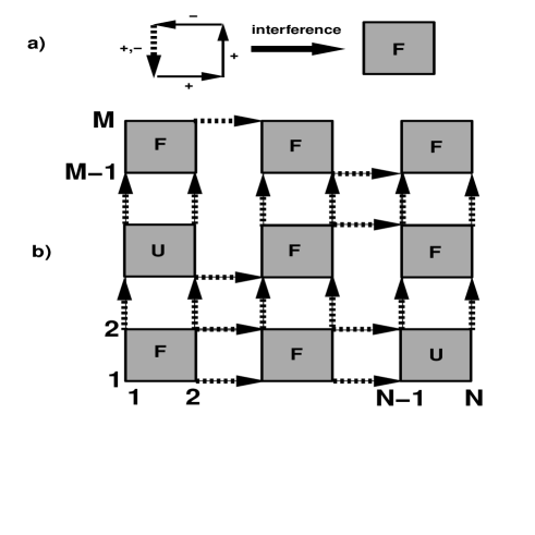
FIG. 3.: a) Preparation of a single plaquette by three $S$ operators (ferro (+), ferro, antiferro (-)) and closing with $\Omega$. This is followed by an interference transformation which erases the antiferromagnetic subspace, leaving in this case a frustrated (F) plaquette. b) A lattice with full density of prefabricated plaquettes (some unfrustrated – U), connected by $\Omega$ operators (dashed arrows), before measurement of the bonds. In this case all vertical bonds are present and the lattice is diluted in the horizontal bonds.

REFERENCES

- [1] P.W. Shor, in Proceedings of the 35th Annual Symposium on the Foundations of Computer Science, edited by S. Goldwasser (IEEE Computer Society, Los Alamitos, CA, 1994), p. 124.
- [2] A. Barenco, Contemp. Phys. 37, 375 (1996).
- [3] A. Ekert and R. Jozsa, Rev. Mod. Phys. 68, 733 (1996).
- [4] D.P. DiVincenzo, Science 270, 255 (1995).
- [5] W.H. Zurek, Physics Today 44 (10), 36 (1991).
- [6] In fact a quantum computer which is only allowed to use superposition, without interference, is equivalent in computational power to a classical probabilistic computer (D. Aharonov, private communication).
- [7] D.P. DiVincenzo, Phys. Rev. A 50, 1015 (1995).
- [8] T. Sleator and H. Weinfurter, Phys. Rev. Lett. 74, 4087 (1995).
- [9] S. Lloyd, Phys. Rev. Lett. 75, 346 (1995).
- [10] D. Deutsch, A. Barenco, and A. Ekert, Proc. Roy. Soc. London Ser. A 449, 669 (1995).
- [11] J.I. Cirac and P. Zoller, Phys. Rev. Lett. 74, 4091 (1995).
- [12] Q.A. Turchette, C.J. Hood, W. Lange, H. Mabuchi and H.J. Kimble, Phys. Rev. Lett. 75, 4710 (1995).
- [13] A. Barenco and A. Ekert, Acta Phys. Slovaca 45, 1 (1995).
- [14] M. Brune, P. Nussenzveig, F. Schmidt-Kaler, F. Bernardot, A. Maali, J.M. Raimond and S. Haroche, Phys. Rev. Lett. 72, 3339 (1994).
- [15] P.W. Shor, Phys. Rev. A 52, 2493 (1995).
- [16] A.M. Steane, Phys. Rev. Lett. 77, 793 (1996).
- [17] A.R. Calderbank and P.W. Shor, Phys. Rev. A 54, 1098 (1996).
- [18] A. Ekert and C. Macchiavello, Phys. Rev. Lett. 77, 2585 (1996).
- [19] R. Laflamme, C. Miquel, J.P. Paz and W.H. Zurek, Phys. Rev. Lett. 77, 198 (1996).
- [20] C.H. Bennett, D.P. DiVincenzo, J.A. Smolin and W.K. Wootters, Mixed State Entanglement and Quantum Error Correction, LANL preprint quant-ph/9604024, submitted to Phys. Rev. A.
- [21] D. Aharonov and M. Ben-Or, Fault tolerant quantum computation with constant error, LANL preprint quant-ph/9611025).
- [22] A. Peres, Error correction and symmetrization in quantum computers, LANL preprint quant-ph/9611046, to appear in Physica D (1997).
- [23] C.H. Bennett, E. Bernstein, G. Brassard and U.V. Vazirani, Strengths and Weaknesses of Quantum Computing, 1997, LANL preprint quant-ph/9701001, to appear in SIAM Journal on Computing.
- [24] R.P. Feynman, Int. J. Theor. Phys. 21, 467 (1982).
- [25] S. Lloyd, Science 273, 1073 (1996).
- [26] B.M. Boghosian and W. Taylor IV, A Quantum Lattice-Gas Model for the Many-Particle Schrödinger Equation in Dimensions, LANL preprint quant-ph/9604035.
- [27] B.M. Boghosian and W. Taylor IV, Simulating Quantum Mechanics on a Quantum Computer, LANL preprint quant-ph/9701019.
- [28] S. Wiesner, Simulations of Many-Body Quantum Systems by a Quantum Computer, LANL preprint quant-ph/9603028.
- [29] C. Zalka, Efficient Simulation of Quantum Systems by Quantum Computers, LANL preprint quant-ph/9603026, submitted to Phys. Rev. A.
- [30] D.A. Meyer, J. Stat. Phys. 85, 551 (1996).
- [31] R. Schak (unpublished).
- [32] H.E. Stanley, Introduction to Phase Transitions and Critical Phenomena (Oxford University Press, Oxford, 1971).
- [33] J.J. Binney, N.J. Dowrick, A.J. Fisher and M.E.J. Newman, The Theory of Critical Phenomena: An Introduction to the Renormalization Group (Clarendon Press, Oxford, 1992).
- [34] N. Metropolis, A. W. Rosenbluth, M.N. Rosenbluth, A.H. Teller and E. Teller , J. Chem. Phys. 21, 1087 (1953).
- [35] S.F. Edwards and P.W. Anderson, J. Phys. F 5, 965 (1975).
- [36] E. Ising, Z. der Physik 31, 253 (1925).
- [37] L. Onsager, Phys. Rev. 65, 117 (1944).
- [38] H.S. Green and C.A. Hurst, Order-Disorder Phenomena (Interscience Publishers, London, 1964).
- [39] R.H Swendsen and J.-S. Wang, Phys. Rev. Lett. 58, 86 (1987).
- [40] G. Toulouse, Commun. Phys. 2, 115 (1977).
- [41] S. Kirkpatrick, Phys. Rev. B 16, 4630 (1977).
- [42] M. Mezard, G. Parisi, and M.A. Virasoro, Spin Glass Theory and Beyond, World Scientific Lecture Notes in Physics (World Scientific, Singapore, 1987).
- [43] K. Binder and A.P. Young, Rev. Mod. Phys. 58, 801 (1986).
- [44] S. Kirkpatrick, C.D. Gelatt, Jr., and M.P. Vecchi, Science 220, 671 (1983).
- [45] F. Barahona, J. Phys. A 15, 3241 (1982).
- [46] G. Parisi, Physica A 140, 312 (1986).
- [47] Y. Fu and P.W. Anderson, J. Phys. A 19, 1605 (1986).
- [48] P.W. Anderson, Physica A 140, 405 (1986).
- [49] D. Kandel, R. Ben-Av and E. Domany, Phys. Rev. Lett. 65, 941 (1990).
- [50] The “” superscript indicates the ferromagnetic case.
- [51] should be understood as “S-plus-J” or “S-minus-J” – not “ to the power ”.
- [52] R. von Mises, Mathematical Theory of Probability and Statistics (Academic Press, New York, 1964).
- [53] Although one should keep in mind that the number of bits required for a desired accuracy of the computation must remain [1, 23].
- [54] This operator is still “valid”, since it can be decomposed into a product of two-qubit operators.
- [55] D.A. Lidar and O. Biham (unpublished).
- [56] Suppose, without loss of generality, that . Then: . For the other direction, take . This proves Eq.(100).
- [57] B.D. Hughes, Physica A 134, 443 (1986).
- [58] N.IA. Vilenkin and A.U. Klimyk, Representation of Lie groups and special functions (Kluwer Academic Publishers, Dordrecht, 1991), Vol. 2, p. 10.
- [59] G.K. Kostopoulos, Digital Engineering (John Wiley & Sons, New York, 1975).
- [60] Technically this is an induction on a finite set, since the lattice is finite. But this is not a problem, since once the entire lattice is covered the operation of closing a new bond is undefined.
- [61] R.J. Baxter, Exactly Solved Models in Statistical Mechanics (Academic, New York, 1982).
- [62] R.J. Baxter, Commun. Math. Phys. 88, 185 (1983).
- [63] V.V. Bazhanov and R.J. Baxter, J. Stat. Phys. 69, 453 (1992).
- [64] M. Suzuki, Phys. Rev. Lett. 28, 507 (1972).
- [65] H.Y. Huang, V. Popkov, and F.Y. Wu, LANL preprint cond-mat/9610184.
- [66] I. Morgenstern and K. Binder, Phys. Rev. B 22, 288 (1980).