Beyond Uncertainty:
the internal structure of electrons and photons

Abstract

The wave–structure of moving electrons is analyzed on a fundamental level by employing a modified de Broglie relation. Formalizing the wave–function $\psi$ in real notation yields internal energy components due to mass oscillations. The wave–features can then be referred to physical waves of discrete frequency $\nu$ and the classical dispersion relation $\lambda\,\nu=u$, complying with the classical wave equation. Including external potentials yields the Schrödinger equation, which, in this context, is arbitrary due to the internal energy components. It can be established that the uncertainty relations are an expression of this, fundamental, arbitrariness. Electrons and photons can be described by an identical formalism, providing formulations equivalent to the Maxwell equations. The wave equations of intrinsic particle properties are Lorentz invariant considering total energy of particles, although transformations into a moving reference frame lead to an increase of intrinsic potentials. Interactions of photons and electrons are treated extensively, the results achieved are equivalent to the results in quantum theory. Electrostatic interactions provide, a posteriori, a justification for the initial assumption of electron–wave stability: the stability of electron waves can be referred to vanishing intrinsic fields of interaction. The concept finally allows the conclusion that a significant correlation for a pair of spin particles in EPR–like measurements is likely to violate the uncertainty relations.

I Introduction

I would like to revive, from a new viewpoint, a somewhat old fashioned discussion, which recently seems to be all but extinct. As goes without saying, every contribution, correction, criticism or suggestion is greatly appreciated.

The discussion, which lasted for the major part of the early stages of atomic, nuclear and particle physics, as we know them today, dealt primarily with the scientific and logical implications of quantum theory. Again revived by David Bohm’s contribution, the “hidden variables”, it gradually began to loose on impact, until today any fundamental question in this respect seems to be considered a lack of scientific soundness.

From an epistemological point of view, the fact is not easily understood, since all the fundamental problems are still far from any solution. Second quantization, on the contrary, provides an even more problematic conception by its inherent infinity problems [1], which, till now, have not been solved in a satisfying way.

That all the original problems are still there, can be seen by a survey of late publications of Bohm [2], de Broglie [3], Dirac [4], or Schrödinger [5].

From the viewpoint of common sense the most profound reason of uneasiness with quantum theory, despite its indisputable successes, has been expressed by Richard Feynman: You see, my physics students don’t understand it either. That is, because I don’t understand it. Nobody does. [6]

That the discussion, mentioned above, is nevertheless non–existent, might have its origins therefore not so much in a satisfying status quo, but rather in a lack of alternative concepts. From an epistemological point of view a well working theory, despite all its conflicts with logical reasoning, is better than no theory. The discussion then leads to the question, why so far no promising concept has been put forth. Comparing with other sciences, the situation seems very unusual: seventy years of continuous research – from Schrödinger’s first publications [7] – have neither altered the principles of quantum theory, nor have they removed the axiomatic qualities of its fundamental statements. This situation basically leaves two possibilities: either to accept, that we cannot understand, i.e. that we have to believe, or to search for alternatives.

The attempts so far, to remove the axiomatic qualities of quantum theory, which can be summarized by the Copenhagen interpretation [9], mainly focussed on the statistical qualities attributed to fundamental physical events. It was thought, that a suitable theoretical framework could prove quantum events to be integral results of basically continuous processes.

The first of these attempts can be attributed to Erwin Schrödinger [7, 8]. His wave mechanics, now a fundamental part of quantum theory, does not allow for an interpretation of wave–functions as physical waves due to the contradiction a spreading wave–packet presents to mass conservation. On a fundamental level, the contradiction originates in the difference between phase velocity and group velocity of de Broglie waves [10]. Since Schrödinger’s equation is based on exactly these qualities of de Broglie waves, it cannot be retained without rejecting the interpretation of wave–functions as physical waves. The problem was solved by Born’s interpretation [11] of $|\psi|^{2}$ as a probability amplitude, an interpretation which constitutes an integral part of the Copenhagen interpretation.

This interpretation of the wave–function is not without its inherent problems, as Einstein, Podolksky and Rosen pointed out [12]. If quantum theory contained all the physical information about a spin–system, thus their line of reasoning, then information about a measurement process must be exchanged with a velocity faster than c, if spin conservation is to be retained. This leaves, as they point out, only two alternatives: either quantum theory contradicts the theory of relativity, or it does not contain all the information about the system: in this case, quantum theory is incomplete. The scientific controversy was subject to much discussion, but never conclusively solved. Recently, its implications have been extended by the phenomenon of ”interaction–free” measurements [13], based on a thought experiment by Renninger [14] and realized by a Mach–Zehnder interferometer. Interaction free measurements have different implications in a classical or quantum context: while a measurement without interaction in classical physics does not alter the system, it leads to a reduction of the wave function in quantum theory. According to the solution, proposed by Heisenberg (see ref.[14]) only the reduction of the wave–function constitutes physical reality: in this case the question is legitimate, why a wave function, obviously devoid of any physical meaning, plays such an important role in current theories.

David Bohm’s famous theory of ”hidden variables” [15] was a far more elaborate concept along the same lines. He tried to prove, that the formalism of quantum theory allows for a sub–layer of hidden variables, and that the framework therefore is, as Einstein suspected, incomplete. The modification was rejected due to the work of Bell, who devised a simple situation, where this assumption could be put to a test [16]. The ”Bell inequalities” proved that, within the framework of quantum theory, such an assumption leads to logical contradictions. The theory of hidden variables was therefore rejected.

The combined evidence of all these attempts allows the conclusion, that a modification of quantum theory within its fundamental axioms, yielding a framework of which the quantum aspect will be but a result, is not very promising. At best, it reproduces numerical results by a different mathematical structure, at worst, it not even accounts for basic experiments. There remain, therefore, three fundamental questions to be answered prior to any attempted modification of micro physics:

• On what theoretical or experimental basis could an alternative formulation be based?

• Which theoretical concept of physics, statistical, field–theory, or mechanics, shall be employed?

• What constitutes a successful alternative to current formulations ?

Experimental evidence exists, that moving electrons exhibit wave–like features. These qualities have been established beyond doubt by diffraction experiments of Davisson and Germer [17]. Quantum theory cannot directly access wave like qualities, because, as already mentioned, the periodic wave function needs to be subjected to a complicated evaluation process in order to extract its physical relevance. If the initial problems of wave dispersion and velocity can be overcome, the experimental result of wave characteristics of moving mass and its mathematical formalization may well constitute the foundation of a different theoretical conception. The only other experimental evidence at hand with equivalent significance, the quantum phenomena, do not as easily fit into a physical interpretation, since the basic obstacle, why discrete values should be the only ones measured, has to be removed: quantum phenomena are therefore more remote in terms of basic concepts.

Concerning the theoretical context, it has to be considered, that quantum theory originally started as a modification of mechanics. Most of the concepts of the theory are consequently still disguised mechanical concepts. Field theoretical results are therefore only achieved by a statistical superstructure: the mechanical basis then leads to a statistical formulation of field theories, which allows for particle interactions, but not for internal particle structures. Modifications of this methodology basically occur along two lines: either by a modification of interactions, which requires additional qualities of particles, or by postulating the existence of sub–particles. Physical progress then requires an ever refined toolkit of particles, sub–particles and interactions. From the viewpoint of epistemology, the problem inherent to this approach is the limited degree of freedom. Every modification requires a major change of particle properties, and since every new experiment provides data not yet accounted for, the development of physics becomes an ever increasing inventory of individual particles. The ”particle–zoo”, high energy physicists so frequently refer to, can, along these epistemological lines, be seen as a consequence of theoretical shortcomings.

Since the experimental basis – the wave characteristics and thus the internal structure of particles – suggest an approach based on field theory rather than mechanics, this essay will be based on field theory. If mechanical concepts are required, they always refer to continuous distributions of physical qualities, which yield discrete mass or charge values only by integration.

If one is to try an alternative route of theoretical development, it seems important, not to get carried away and extend a concept beyond its limits of proper application. To this end, a goal has to be defined as well as careful checks of experimental evidence. A theory, which does not allow for falsification, remains useless, the same applies to a new theory, which does not deviate from the current one by at least one significant result. That a new theory cannot – and should not – reproduce all results of an existing one, goes without saying. Personally, I think that the following results are sufficient to justify serious consideration of a new approach:

• The reproduction of fundamental results of early quantum theory

• The formalization of internal particle structures and the proof of physical significance of these structures

• A model of (hydrogen) atoms consistent with the formalism developed and consistent with experimental evidence

• The basics of a theory of particle–interaction due to intrinsic characteristics

• Provision of at least one significant deviation which allows for an experimentum crucis

The fundamental relations and concepts of this new approach have already been published or are in print in the Speculations in Science and Technology (Chapman and Hall, London) [18, 19]. The accounts given in this and follow–up papers are somewhat enhanced and thorougher versions, making use of the greater freedom of length. As already emphasized, any feedback is greatly appreciated and readers are welcomed to contact me directly via email at the email address: whofer@eapa04.iap.tuwien.ac.at

II Wave structure

To allow for internal characteristics of moving particles we base the following section on the experimental evidence of wave–features. Theoretically, the framework will be based on a suitable adaptation of the fundamental relations found by L. de Broglie. Originally, de Broglie’s formalization of waves [10] was based on the framework of Special Relativity, the amplitude of a ”de Broglie wave” given by:

$$\psi(x_{\mu})=\psi_{0}\exp\,-i\left(k^{\mu}x_{\mu}\right)$$ (1)

The variables are four–dimensional vectors, their components are described by the following relations:

$$x_{\mu}=(ct,-x,-y,-z)\qquad k^{\mu}=\frac{m\gamma}{\hbar}\left(c,u_{x},u_{y},u_{z}\right)$$ (2)

In a three dimensional and non–relativistic ($\gamma$ = 1) adaptation of the original equation (1) the amplitude can be expressed as a plane wave. This adaptation is quite common in quantum theory and therefore no deviation from the original framework:

$$\psi(\vec{x},t)=\psi_{0}\exp\,i\left(\frac{m\,\vec{u}}{\hbar}\vec{x}-\omega t\right)$$ (3)

The first major deviation from the traditional framework is the interpretation of $\psi(\vec{x},t)$ as a real function, as a physical wave. This conception is not compatible with quantum theory for the following reasons: as a moving particle cannot consist of a specific plane wave (particle mass in this case would be distributed over an infinite region of space), a moving particle in quantum theory must be formalized as a Fourier integral over partial waves. An application of Schrödinger’s equation then leads to the, above mentioned, spreading of the wave–packet, which contradicts experimental evidence. The interpretation of the wave–function as a physical entity, furthermore, contradicts Heisenberg’s uncertainty relation [20], because it implies the possibility of measurements below quantum level.

$$\psi(\vec{x},t)=\psi_{0}\sin\left(\frac{m\,\vec{u}}{\hbar}\vec{x}-\omega t\right)\qquad\psi_{0}\in\,R$$ (4)

The reason, that this–real–formalization of de Broglie remained so far unconsidered, is not only its inconsistency with quantum theory, but also a consequence of Planck’s relation: dispersion of de Broglie waves is described by two independent relations, which are widely confirmed in experiments. The first is the wavelength of de Broglie waves, established by diffraction experiments of Davisson and Germer [17], the second Planck’s energy relation [21]:

$$\lambda(\vec{p})=\frac{h}{|\vec{p}|}\qquad E(\omega)=\hbar\,\omega$$ (5)

If particle energy is classical kinetic or relativistic energy, the phase velocity of a de Broglie wave is not equivalent to particle velocity:

$$\hbar\omega=E\quad\Longrightarrow\quad c_{phase}=\frac{\omega}{k}=\left\{\frac{c^{2}}{u}\right\}_{rel}=\left\{\frac{u}{2}\right\}_{non-rel}$$ (6)

The deduction of phase velocity, leading to the contradiction in Eq. (6) is, contrary to a first impression, not self–evident. It contains, on thorougher analysis, a conjecture and a subsequent logical circle. Firstly, it is not self–evident, that on a micro–level energy of a particle is restricted to kinetic energy of inertial mass: assuming, that a particle is, basically, a mechanical entity without any internal energy component, cannot be inferred from experimental or theoretical results. It is therefore an assumption lacking a solid basis. Based on this conjecture is the following logical circle:

If energy is kinetic energy, phase velocity of a de Broglie wave is not equal to mechanical velocity of a particle. If phase velocity does not equal mechanical velocity, a free particle cannot consist of a single wave of specific frequency. If it does not consist of a single wave, then the wave–features of a particle must be formalized as a Fourier integral over infinitely many partial waves. In this case any partial wave cannot be interpreted as a physical wave. If the interpretation as a physical wave is not justified, then internal wave–features cannot be related to physical qualities. If they cannot be related to physical qualities, then internal processes must remain unconsidered. And if internal processes remain unconsidered, then energy of the particle is kinetic energy

Apart from the question, whether this assumption is necessary, which can only be answered a posteriori, it seems also legitimate to ask, whether it is the best possible assumption, especially in view of complications arising from fundamental particles formalized as Fourier integrals over infinitely many partial waves. From the viewpoint of simplicity, the concept is necessary, if no alternative exists, it is unnecessary complicated, if the same theoretical result – the wave features of single particles – can be obtained by a simpler formalism. To this aim alternatives have to be analyzed. A direct way of formalization would be based on two basic statements: (1) the experimental evidence of wave features, and (2) the assumption, that wave features must be reflected by physical qualities of particles, density for example. Mathematically, these statements are expressed by:

$$\psi(\vec{x},t)=\psi_{0}\sin\left(\frac{m\vec{u}}{\hbar}\vec{x}-\omega t\right)$$ (7)

$$\rho(\vec{x},t)=C\,\psi_{0}^{2}\sin^{2}\left(\frac{m\vec{u}}{\hbar}\vec{x}-\omega t\right)$$ (8)

In view of the dispersion relations Eq. 5 these relations seem contradictory: the standard evaluation procedure would, for a specific physical wave, lead to a difference between phase velocity and mechanical velocity in conflict with the energy principle.

A Kinetic and potential energy

This contradiction depends, though, on the principal conjecture, that a moving particle is equivalent to inertial mass, and that all its energy is contained in the – longitudinal – motion of an inertial mass $m$ with velocity $|\vec{u}|$. As soon as wave features are assumed to describe the physical nature of particle motion, this conjecture can no longer be sustained: energy of the particle will then be contained in its mass oscillations.

Since mass oscillations determine a periodic change of kinetic energy, the energy principle requires the existence of an intrinsic potential of particle motion, and averaging over kinetic and potential energy during particle motion then leads to a total energy of double the original kinetic value. Using this total energy for Planck’s relation satisfies the dispersion relation of a monochromatic plane wave: based on the intrinsic properties of physical waves any monochromatic plane particle wave then satisfies the wave equation. Averaging density of the particle wave over a full period we get initially:

$$\int_{0}^{\lambda}\rho(\vec{x},t=0)d|\vec{x}|=\frac{C}{2}\,\psi_{0}^{2}\lambda=:\bar{\rho}\,\lambda$$ (9)

$$\bar{\rho}=\frac{C}{2}\,\psi_{0}^{2}$$ (10)

And the kinetic energy of particle motion is therefore ($V_{P}$ denotes the volume of the particle):

$$W_{K}=V_{P}\,\frac{\bar{\rho}}{2}|\vec{u}|^{2}=\frac{m}{2}\,|\vec{u}|^{2}$$ (11)

Since kinetic energy is not constant but periodic, the result requires that an intrinsic potential exists, which yields an equivalent average of potential energy:

$$W_{P}=V_{P}\,\frac{\bar{\rho}}{2}|\vec{u}|^{2}=\frac{m}{2}\,|\vec{u}|^{2}$$ (12)

And total energy of the particle wave is then:

$$W_{T}=W_{K}+W_{P}=m\,|\vec{u}|^{2}=:\hbar\,\omega$$ (13)

Phase velocity of this particle wave equals, consistent with quantum theory, mechanical velocity of particle motion, although, contrary to quantum theory, no Fourier integral over partial waves is required. Therefore any monochromatic plane particle wave, consisting of oscillating mass and a complementary potential, describes motion of a free particle:

$$c_{ph}=\frac{\omega}{|\vec{k}|}=\lambda\,\nu=\frac{m\,|\vec{u}|^{2}}{m\,|\vec{u}|}=|\vec{u}|$$ (14)

From a theoretical point of view the existence of intrinsic potentials is a conjecture, it is more problematic than the original one based on inertial mass, since it implies the existence of physical variables not accounted for in the current framework of quantum theory. Relating $\hbar\omega$ to total energy of the particle is, in this respect, not problematic, since experimentally energy of a particle can only be estimated by its state of motion or wavelength: and the relation between particle velocity $\vec{u}$, wavelength $\lambda$, and frequency $\omega$ is retained.

B Wave equation

With the dispersion relation given by Eq. 14 the wave function $\psi(\vec{x},t)$ and density $\rho(\vec{x},t)$ of free particles comply with a wave equation:

$$\triangle\,\psi(\vec{x},t)-\frac{1}{c_{ph}^{2}}\frac{\partial^{2}\psi(\vec{x},t)}{\partial t^{2}}=0$$ (15)

$$\triangle\,\rho(\vec{x},t)-\frac{1}{c_{ph}^{2}}\frac{\partial^{2}\rho(\vec{x},t)}{\partial t^{2}}=0$$ (16)

The wave equations display intrinsic features of particle motion and possess, as will be seen in the following sections, the same dimensional level as electrodynamic formulations. The logical structure of physical statements is therefore modified: while in the standard procedure of quantum field theory the fundamental statements of quantum theory determine events on a micro level, and electromagnetic fields are logical superstructures, in the present context statements about the wave features of particles are different aspects of the same physical phenomena dealt within electrodynamics.

This parallel development of electrodynamics and quantum theory from the same root – the intrinsic wave features of particles – must be understood in a literal sense, because the potentials deduced from mass oscillations will be related to electromagnetic fields.

C Schrödinger equation

The Schrödinger equation, in this context, is an expression of mechanical features – i.e. potential and kinetic energy – of particle motion. From the viewpoint of physical waves it is not without a certain degree of arbitrariness. To derive the relation we proceed from the periodic wave function Eq. 14. Then the time differential is given by:

$$|\vec{u}|^{2}\,\triangle\psi=\frac{\partial^{2}\psi}{\partial t^{2}}=-\omega^{2}\,\psi$$ (17)

Kinetic energy $W_{K}$ of particle motion will therefore be:

$$W_{K}\psi=\frac{m}{2}\,|\vec{u}|^{2}\,\psi=\frac{\hbar}{2}\,\omega\,\psi$$ (18)

And substituting Eq. 17 into 18 we get for the kinetic energy of the particle:

$$\left(W_{K}+\frac{\hbar^{2}}{2m}\triangle\right)\psi=0$$ (19)

$$W_{K}=-\frac{\hbar^{2}}{2m}\triangle$$ (20)

If the total energy of a particle is equal to kinetic energy and a potential $V(\vec{r})$:

$$W_{T}=V(\vec{r})+W_{K}$$ (21)

then the wave equation in the presence of an external potential is described by:

$$\left(-\frac{\hbar^{2}}{2m}\triangle+V(\vec{r})\right)\psi=W_{T}\,\psi$$ (22)

The relation is equivalent to a time–free Schrödinger equation [7]. It is important to consider, that this (mechanical) formulation of the wave equation explicitly relates physical potentials to kinetic energy and thus the wave–length of a material wave (as a result of the Laplace operator acting on $\psi$) and that, therefore, in a region, where $V(\vec{r})$ takes successively different values, every kinetic energy and thus wave–length is generally possible.

Its interpretation in the context of material waves is not trivial, though. If the volume of a particle is finite, then wavelength and frequency become intrinsic variables of motion, which implies, due to energy conservation, that the wave function itself is a measure for the potential at an arbitrary point $\vec{r}$. If it is a measure for the physical conditions of the environment – i.e. the intensity of $V(\vec{r})$ –, then it must have physical relevance. But if it has physical relevance, then the EPR dilemma [12] will be fully confirmed, and the result will favor Einsteins’s interpretation of quantum theory: quantum theory cannot be complete under the condition that (1) particles do have finite dimensions, and (2) the Schrödinger equation is a correct description of the variations of particle waves in the presence of external fields. The only alternative, which leaves quantum theory intact, is the assumption of particles with zero volume: an assumption which leads, in the context of electrodynamics, to the equally awkward result of infinite energy of particles. The first major result of this essay can therefore be formulated as follows:

• The interpretation of particles as physical waves allows the conclusion, that quantum theory cannot be, in a logical sense, a complete theoretical description of micro physical systems.

There exists another problem usually hidden in the mathematical formalism of quantum theory. Let an external potential be given by $V(\vec{r})$. Transforming Eq. 22 into a moving coordinate system $\vec{r}\,^{\prime}$ described by:

$\displaystyle\vec{r}\,^{\prime}=\vec{r}-\vec{u}\,t$

we get the following equation:

$$\left(-\frac{\hbar^{2}}{2m}\triangle^{\prime}+V(\vec{r}\,^{\prime}+\vec{u}\,t)\right)\psi(\vec{r}\,^{\prime})=W_{T}\,\psi(\vec{r}\,^{\prime})$$ (23)

Since the variable $t$ in this case is undefined, the relation contains an element of arbitrariness. It is not conceivable, from this deduction, how a time–free Schrödinger equation could be derived: if the time–dependent part of $\psi$ is eliminated, the procedure is equivalent to a transformation into a moving coordinate system, but in this case the potential becomes a function of time. And if the wave equation is integrated in the system at rest, then the wave functions depend on time.

From a physical point of view, the reduction of the Schrödinger equation to its time–free form actually eliminates all the time–dependent interaction and adjustment processes bound to occur for every particle wave interacting with a changed environment. It may well be, that this disregard of development accounts for the commonly rather static concepts in quantum theory.

D Uncertainty Relations

Within the framework of material waves, the arbitrariness of the Schrödinger equation can be referred to the intrinsic potential of mass oscillations, not accounted for in quantum theory. And its consequence, as can equally be derived, is an uncertainty about the exact value of $\vec{k}$ of the wave function $\psi(\vec{k},\vec{r})$. The uncertainty of $\vec{k}$ together with the period of intrinsic potentials $\phi$ is then sufficient to derive Heisenberg’s uncertainty relations [20, 22]. To this aim we proceed from the Schrödinger equation in the moving frame of reference Eq. 23. Setting the upper and lower limits of the potential $V(\vec{r}^{\prime}+\vec{u}t)$ to:

$\displaystyle V_{1}=V(\vec{r}^{\prime}+\vec{u}t_{1})\quad V_{0}=V(\vec{r}^{\prime}+\vec{u}t_{0})$

and calculating the correlating $k$–vectors of the wave function $\psi(\vec{r}^{\prime},\vec{k})$:

$\displaystyle\psi(\vec{r}^{\prime},\vec{k}):=\psi_{0}e^{i\vec{k}\vec{r}^{\prime}}$

we get the following relation:

$$\hbar^{2}(\vec{k}_{1}^{2}-\vec{k}_{0}^{2})+2m(V_{0}-V_{1})=0$$ (24)

$$\vec{k}_{1}=\vec{k}_{1}(\vec{r}^{\prime},t)\quad\vec{k}_{0}=\vec{k}_{0}(\vec{r}^{\prime},t)$$ (25)

Evaluating the relation in a one–dimensional model and accounting for the – yet unknown – variation of the potential $V$ by:

$$V_{1}(\vec{r}^{\prime},t) = V(\vec{r}^{\prime})+\triangle V(t)\quad V_{0}(\vec{r}^{\prime},t)=V(\vec{r}^{\prime})-\triangle V(t)$$ (26)

$$k_{1}(\vec{r}^{\prime},t) = k(\vec{r}^{\prime})+\triangle k(t)\quad k_{0}(\vec{r}^{\prime},t)=k(\vec{r}^{\prime})-\triangle k(t)$$ (27)

the uncertainty $\triangle k$ due to the undefined variable t will be:

$$\hbar\triangle k(t)=\frac{m\,\triangle V(t)}{\hbar k}$$ (29)

If the uncertainty originates from the neglected intrinsic potential $W_{P}$ (see Eq. 12), the uncertainty of the applied potentials is described by:

$$\phi_{0}=mu^{2}=\triangle V$$ (30)

And therefore the uncertainty of $k$ can be referred to the value of $k$:

$$\hbar\triangle k=\frac{m\,\phi_{0}}{\hbar k}=mu=\hbar k$$ (31)

The uncertainty does not result from wave–features of particles, as Heisenberg’s initial interpretation suggested [22], nor is it an expression of a fundamental physical principle, as the Copenhagen interpretation would have it [9]. It is, on the contrary, an expression of the minimum error, inherent to any evaluation of the Schrödinger equation, resulting from the fundamental assumption in quantum theory, i.e. the interpretation of particles as inertial mass aggregations.

Since the distance between two potential maxima is given by (the value can deviate in two directions which yields total uncertainty of the $x$–coordinate):

$$\triangle x=\frac{\lambda}{2}=2(x(\phi_{0})-x(0))$$ (32)

the uncertainty may equally be written as:

$$\triangle k\triangle x\geq\frac{k\lambda}{2}\qquad\triangle p\triangle x\geq\frac{h}{2}$$ (33)

Heisenberg actually derived [22] the uncertainty relations $\triangle p\triangle q=\hbar$. The Fourier transform inherent to quantum theory suggests a correction of the constant Eq. 33 by a factor $(2\pi)^{-1}$. In this case the deduction yields exactly the same result as the canonical formulation of quantum theory [23]:

$$\triangle X_{i}\,\triangle P_{i}\geq\frac{\hbar}{2}$$

The minimum error due to intrinsic potentials is therefore equal to the uncertainty of quantum theory, and the logical relation between Schrödinger’s equation and the uncertainty relations is therefore a relation of reason and consequence: Because Schrödinger’s relation is not precise by the value of intrinsic potentials, the uncertainty relations must be generally valid. This is the second major result of the present essay:

• Because quantum theory neglects intrinsic characteristics of particle motion, the Schrödinger equation is generally not precise by a value described by Heisenberg’s uncertainty relations.

The result equally seems to settle the long–standing controversy between the empirical and the axiomatic interpretation of this important relation: it is not empirical, since it does not depend on any measurement process; but it is equally not a physical principle, because it is due to the fundamental assumptions of quantum theory. The solution to the problem of interpretation is therefore a somewhat wider frame of reference: although within the principles of quantum theory the relation is an axiom, it is nonetheless a result of fundamental theoretical shortcomings and not a physical principle.

E Summary

In the preceding section we could demonstrate, that quantum theory must not necessarily be a comprehensive representation of physical reality. It was shown, on the contrary, that the principal assumption of quantum theory, the assumption of inertial mass of particles, is a posteriori neither justified by the wave features of particles nor by the fundamental Planck and de Broglie relations. It is but one possible theoretical framework and, given the logical problems of a precise relation between measurements and reality arising from this concept, not even the best possible framework.

On an analytical level the establishment of fundamental relations of quantum theory within a different framework and their significance – that the uncertainty relations can also, and consistently, be interpreted as an expression of theoretical shortcomings due to a disregard of intrinsic properties – served to establish the limitations of the current theoretical standard. They also served to define the logical location of quantum theory and to determine the regions of interest, where research is commendable if a theory outside the current framework is taken into consideration.

From the viewpoint of theoretical synthesis we showed that the intrinsic properties of particles and their relations are a consequence of the experimental evidence of wave–features of particles. The de Broglie relations, in a non–relativistic formulation, provided the essential laws by which these intrinsic variables are described. They allowed to establish (1) periodic mass–oscillations within the particle, and (2) the existence of a periodic potential. These results were sufficient to deduce the fundamental relations of quantum theory and, at the same time, to show their inherent limitations. Apart from showing the significance of the periodic potentials – which will be done in the following sections – the first two requirements mentioned in the introduction are therefore fulfilled. Fundamental results of early quantum theory are reproduced (Schrödinger’s relation as well as the uncertainty relations, while single experiments will be treated in the following sections), and the intrinsic wave features of particles were shown to be of physical significance, which strongly supports Einstein’s view in the EPR paradox.

III Classical Electrodynamics

Classical electrodynamics is considered one of the most refined and powerful physical theories at hand. It served, during the last hundred years, ever again as a model for physical formalization, and its implications led to quite a few extensions of physical knowledge, not least Albert Einstein’s theory of Special Relativity [24]. A great deal of the fascination of classical electrodynamics results from its mathematical conciseness and brevity. The possibility to describe and account for most of the phenomena concerning interactions of charge by a set of basically four linear differential equations, the Maxwell equations [25], must either seem a lucky coincidence or an expression of a deeply rooted analogy in physical reality.

That classical electrodynamics cannot be referred to mechanical conceptions, has been proved during the scientific controversy about the existence of the ”Aether”. This proposed medium of electromagnetic fields was never detected, its existence, furthermore, would contradict the experimental results of Michelson and Morley [26]. From the theoretical side, the controversy was settled by Einstein’s theory of relativity. Since the correctness of Maxwell’s equations is established beyond doubt, it remains an epistemological problem, why no attempt to refer them to fundamental physical axioms has succeeded so far [27]. Summarizing the current situation in two statements: (1) Maxwell’s equations are correct, and (2) they cannot be referred to mechanical axioms, there exist equally two logical conclusions to the epistemological problem: (1’) Maxwell’s equations are themselves of an axiomatic nature, and (2’) The axioms, on which they are based, have not yet been detected.

Currently, the established opinion is (1’). Basically, one could leave it at this state and employ the relations as correct algorithms. From the viewpoint of macro physics, the procedure is justified by the wealth of experimental verifications at hand. The same does not apply, though, to an application of electrodynamics in micro physical models. Since the exact origin of the relations is obscure, it cannot be guaranteed, that they do not, in some way, preclude characteristics of physical systems, which contradict other assumptions. Obviously, there exist only two ways out of this logical dilemma: either it can be proved, that quantum theory is logically independent of electrodynamics – a proof, which never has been given –, or it can be established that electrodynamics itself is based on micro physical axioms: in this case the current procedure in QED [1] is logically insufficient. The logical conclusion to our epistemological problem would then be: (2”) The Maxwell relations are an expression of intrinsic characteristics of particles.

A The Maxwell equations

Based on the intrinsic wave characteristics of free particles, developed in the previous section, the verification of (2”) does not present an impossible problem. The Maxwell equations, in material wave theory, are an expression of longitudinal variations of intrinsic variables of particles in motion. From the wave equation for longitudinal momentum $\vec{p}$:

$$\nabla^{2}\,\vec{p}-\frac{1}{u^{2}}\frac{\partial^{2}\,\vec{p}}{\partial t^{2}}=0\quad\vec{p}=\rho\,\vec{u}\quad\vec{u}=\mbox{const}$$ (34)

And the equation of continuity for momentum $\vec{p}$ and density $\rho$:

$$\nabla\,\vec{p}+\frac{\partial\,\rho}{\partial t}=0$$ (35)

it follows within a micro volume, where particle velocity $\vec{u}$ is constant:

$$\nabla^{2}\,\vec{p} = -\nabla\,\frac{\partial\,\rho}{\partial t}-\nabla\times(\nabla\times\vec{p})$$ (36)

$$\frac{1}{u^{2}}\frac{\partial^{2}\,\vec{p}}{\partial t^{2}} = \frac{\partial}{\partial t}\left(\frac{\bar{\sigma}}{u^{2}}\frac{1}{\bar{\sigma}}\frac{\partial\,\vec{p}}{\partial t}\right)$$ (37)

The parameter $\bar{\sigma}$ is a dimensional constant employed to make mechanical units compatible with electromagnetic variables, its dimension is equal to density of charge.

Electric fields $\vec{E}$ and magnetic fields $\vec{B}$ are now defined in terms of momentum $\vec{p}$ and the potential $\phi(\vec{r},t)$ due to mass oscillations (see the previous section):

$$\vec{E} := -\nabla\,\frac{1}{\bar{\sigma}}\phi(\vec{r},t)+\frac{1}{\bar{\sigma}}\frac{\partial\,\vec{p}}{\partial t}$$ (38)

$$\vec{B} := -\frac{1}{\bar{\sigma}}\nabla\times\vec{p}$$ (39)

And substituting Eq. 36 into 34 we get, with the help of 38 and 39:

$$\frac{\partial}{\partial t}\,\nabla\left(\frac{1}{u^{2}}\,\phi+\rho\right)+\bar{\sigma}\left(\frac{1}{u^{2}}\frac{\partial\vec{E}}{\partial t}-\nabla\times\vec{B}\right)=0$$ (40)

And since the total intrinsic potential is a constant:

$$\phi(\vec{r},t)+\rho(\vec{r},t)\,u^{2}=\phi_{0}=\mbox{const}$$ (41)

The following relation holds in full generality within every micro volume:

$$\frac{1}{u^{2}}\frac{\partial\vec{E}}{\partial t}=\nabla\times\vec{B}$$ (42)

Rotation of Eq. 38 yields, but for a constant, Maxwell’s first equation:

$$\nabla\times\vec{E}=\frac{1}{\bar{\sigma}}\frac{\partial}{\partial t}\nabla\times\vec{p}=-\frac{\partial\vec{B}}{\partial t}$$ (43)

To deduce the inhomogeneous equation we additionally have to employ the source equations of electrodynamic theory and the definition of $\vec{H}$ fields:

$$\nabla(\epsilon\vec{E})=\nabla\vec{D}=\sigma\quad\nabla\vec{B}=0$$ (44)

$$\nabla J(\vec{r},t)=-\frac{\partial\sigma}{\partial t}$$ (45)

$$\vec{H}=\mu^{-1}\,\vec{B}$$ (46)

It is assumed that the material constants $\epsilon$ and $\mu$ also remain constant within the micro volume. Substituting into Eq. 42 and computing the source of 45, the sum yields:

$$\nabla\left(-\frac{1}{u^{2}}\frac{\partial\mu^{-1}\vec{E}}{\partial t}+\frac{\partial\vec{D}}{\partial t}+\vec{J}\right)=0$$ (47)

And if the constant of integration is zero, the result will be Maxwell’s inhomogeneous equation:

$$\vec{J}+\frac{\partial\vec{D}}{\partial t}=\nabla\times\vec{H}$$ (48)

Finally, by computing the time differentials of Eqs. 42 and 43, the wave equations for electromagnetic fields in a vacuum ($\sigma=0$) can be deduced:

$$\nabla^{2}\vec{E}-\frac{1}{u^{2}}\frac{\partial^{2}\vec{E}}{\partial t^{2}}=0$$ (49)

$$\nabla^{2}\vec{B}-\frac{1}{u^{2}}\frac{\partial^{2}\vec{B}}{\partial t^{2}}=0$$ (50)

The results indicate, that electrodynamics and quantum theory do have a common root, the intrinsic properties of moving particles. From the viewpoint of material waves they are therefore different aspects of the same physical phenomenon, the wave features of mass, which is the third major result of this essay:

• Electrodynamics and wave mechanics are theoretical concepts based on the same physical phenomena, the intrinsic features of moving particles.

Logically speaking, the result means, that a method, which employs quantum theory to calculate physical variables by way of observables, and which identifies these observables – measured variables – as field variables in electrodynamics cannot be correct.

B Energy relations

The energy principle of material waves can be identified as the classical Lorentz standard by a combination of the continuity equation and the definition of electric fields including intrinsic potentials. Since:

$$\nabla{\vec{p}}+\frac{\partial\rho}{\partial t}=0\qquad\bar{\sigma}{\vec{E}}=-\nabla\phi+\frac{\partial{\vec{p}}}{\partial t}$$ (51)

the wave equation for linear motion $\nabla\times\nabla\times{\vec{p}}=0$ leads to:

$$\nabla(\nabla{\vec{p}})+\frac{\partial}{\partial t}\nabla\rho=\frac{1}{u^{2}}\frac{\partial^{2}}{\partial t^{2}}{\vec{p}}+\frac{\partial}{\partial t}\nabla\rho$$ (52)

$$\Rightarrow\qquad\frac{\partial{\vec{p}}}{\partial t}+u^{2}\nabla\rho=const=:0$$ (53)

And for uniform motion $\bar{\sigma}{\vec{E}}=0$ the potential can be related to momentum ${\vec{p}}$ by:

$$\frac{1}{u^{2}}\frac{\partial\phi}{\partial t}-\nabla{\vec{p}}=0$$

Comparing with the expression in classical electrodynamics the vector potential $\vec{A}$, in classical electrodynamics an abstract conception, is proportional to momentum of particle motion:

$$\nabla{\vec{A}} +\frac{1}{c}\frac{\partial\phi}{\partial t}=0\qquad-\nabla{\vec{p}}+\frac{1}{u^{2}}\frac{\partial\phi}{\partial t}=0$$ (54)

$${u=c\atop\Rightarrow} \qquad{\vec{A}}=-c\,{\vec{p}}=:\frac{1}{\alpha}\,{\vec{p}}$$ (55)

C Photons

The wave–features of photons, or the representation of electromagnetic fields by wave–type field vectors, have long been the only aspect in consideration. The picture changed only after experimental research was directed towards the fundamental problems of interaction between matter and electromagnetic fields. Due to Planck’s result on black–body radiation and Einstein’s application of Planck’s formula to the problem of photo–electricity [28], the energy of photons gained special attention, since it was (1) proportional to frequency and not, as field theory proposed, intensity, and (2) the energy quantum $\hbar\omega$ could no longer be distributed locally, because the energy changes in interactions required an exchange of a full number $n\in N$ of energy quanta. In Einstein’s view the interaction suggested that energy of photons be distributed in single points within the electromagnetic fields of radiation.

According to the Copenhagen interpretation of quantum theory [9] the two theoretical aspects – wave–features and energy quanta – describe complementary facts of a complex physical reality not adaptable to any single theoretical framework. This interpretation, which focusses on the central notion of wave–particle–duality, states that all the qualities like polarization and interference, typical for a wave–type theory, have to be treated by electrodynamics, while energy and interaction phenomena must be seen from the viewpoint of quantum theory. The logical justification for retaining the duality, which is in itself a logical contradiction if wave–features and particle features were to prevail simultaneously, was seen by Jordan [29] and Heisenberg [30] in the impossibility of experiments – i.e. physical processes – where both aspects must simultaneously exist.

This justification is not undisputed. Renninger showed by a rather simple thought–experiment [31], that an interference measurement involving two separate light–paths does not allow for the probability–interpretation of electromagnetic field vectors, since the result of the measurement can be altered in a deterministic manner by the insertion of optical devices into a single light–path. The analysis of the experiment leads to the conclusion, that the wave–features must have physical significance, which again seems to confirm the EPR dilemma already quoted [12]. Based on this experiment Renninger deduced the following statement about the features of photons (translation by the author, emphasizing by Renninger):

Every light–quantum consists of an energy–particle, which is guided by a wave without energy

The important result, from our point of view, is the physical significance of wave–features. The energy particle, which Renninger refers to, is a direct result of Einstein’s interpretation of photo–electricity, which equally determines the interpretation of the guiding wave as energy–free. From the viewpoint of physical concepts, an energy–free physical wave is not all too convincing. If a region of space is altered by a propagating wave, thus the obvious objection, then it cannot be without a physical entity moving. But since all physical field–variables are, in some way, related to energy, a physical entity propagating without any propagation of energy seems contradictory.

On thorougher analysis the necessity to divide between two separate physical entities to account for energy as well as electromagnetic features of photons depends on the interpretation of the interaction process itself. Since (1) the quantum of energy is fully transferred, and (2) the transfer interval is well below the level of measurements, the energy must be contained in an insignificantly small volume. The alternative being, as Renninger pointed out, that the wave will be contracted with a velocity exceeding $c$ during every interaction process.

It is this interpretation of the interaction process, which will be changed by material wave theory. To understand the decisive modification, we present here – and without proof – a result on the interactions of electrons and photons, which will be derived later on.

Assuming that the interaction interval equals $n\,\tau,n\in N$, and setting $n$ for convenience equal to 1, an intrinsic model of particles and fields will have to consider energy density at a specific point within the particle. If total energy density is constant and $\phi_{0}$, then the time–derivative of energy density equals:

$$\frac{d\phi}{dt} = \frac{\phi_{0}}{\tau}=\frac{\rho u^{2}}{\tau}=\frac{1}{V_{ph}}\,h\nu^{2}$$ (56)

$$\frac{dE_{ph}}{dt} = V_{ph}\frac{d\phi_{0}}{dt}=h\nu^{2}$$ (57)

$$E_{ph} = \int_{0}^{\tau}dt\frac{dE_{ph}}{dt}=h\nu$$ (58)

In this way the traditional features of photons are retained, while the meaning of the term energy quantum is modified: the energy quantum transferred in an interaction process equals $h\nu$, regardless of the actual volume of the photon, and equally regardless of the exact duration of the interaction process. As long as the total density of energy $\phi_{0}$ is constant, the relation holds for every single point of the underlying field and therefore for the whole region of the physical wave corresponding to a photon.

Now let us consider a case, where the initial photon is, by some optical device, split into two. If one of the partial volumes – a half photon so to say – then interacts with matter, the process is described by:

$$\frac{d\phi}{dt} = \frac{\rho u^{2}}{\tau}=\frac{1}{2V_{ph}^{\prime}}\,h\nu^{2}$$ (59)

$$\frac{dE_{ph}^{\prime}}{dt} = V_{ph}^{\prime}\frac{d\phi_{0}}{dt}=\frac{1}{2}h\nu^{2}=\frac{1}{2}\frac{dE_{ph}}{dt}$$ (60)

$$E_{ph}^{\prime} = \int_{0}^{\tau}dt\frac{dE_{ph}^{\prime}}{dt}=\frac{1}{2}h\nu=\frac{1}{2}E_{ph}$$ (61)

The energy density transferred remains constant, but not total energy. The process therefore seems to be a confirmation of the principle, that all interactions occur in discrete energy quanta only, if discrete quantities of mass or charge are considered. Only, in short, if the general outlook on processes is a mechanical one. It is no contradiction with Einstein’s calculation on photo–electricity, to interpret it as an effect of energy densities and transfer rates. It only has to be considered, that the total volume affected by interactions will depend on the total volume of the – fractional – photon.

From this result it can be concluded, that the term energy quantum is not appropriate for the physical process of interaction: since the total energy transferred depends on (1) the frequency of radiation, and (2) the volume of the photon, total energy transferred is the product of energy density – proportional to frequency – and volume – which may be related to intensity. In an intrinsic formalism of interaction, furthermore, the total quantities transferred are only secondary, the more so, since electrodynamics already is a theory of intrinsic wave features, as deduced above.

In material wave theory photons are distributions of mass and energy, and the guiding wave possesses the same dimensions as the energy distribution, while the guiding wave as well as mass movement contribute alike to total energy of the photon. To derive the essential features of photons we use the fundamental wave equation of intrinsic particle momentum. The exact dimensions as well as the problems of photon boundaries are shown to be of no effect for the results achieved.

Denoting an, initially, abstract momentum of a photon by ${\vec{p}}$, we proceed from the wave equation in a vacuum given by:

$$\nabla^{2}\,{\vec{p}}-\frac{1}{c^{2}}\,\frac{\partial^{2}\,{\vec{p}}}{\partial\,t^{2}}=0$$ (62)

With the identity for the Laplace operator and the general relation between momentum ${\vec{p}}$ and vector potential ${\vec{A}}$ from Eq. ( 55):

$$\nabla^{2}\,{\vec{V}} = \nabla(\nabla\,{\vec{V}})-\nabla\times(\nabla\times{\vec{V}})$$ (63)

$${\vec{p}} = \alpha{\vec{A}}$$ (64)

$$\frac{1}{c}\frac{\partial\,{\vec{p}}}{\partial\,t} = \frac{\alpha}{c}\frac{\partial\,{\vec{A}}}{\partial\,t}\qquad\nabla\times{\vec{p}}=\alpha\,\nabla\times{\vec{A}}$$ (65)

the wave equation may be rewritten as:

$$\nabla(\nabla\,{\vec{p}})-\alpha\,\nabla\times{\vec{B}}-\frac{\alpha}{c}\left(\frac{1}{c}\frac{\partial^{2}\,{\vec{A}}}{\partial\,t^{2}}\right)=0$$ (66)

Using the solution for the homogeneous Maxwell relations (the following deduction employs, for convenience, Gaussian units):

$$\frac{1}{c}\frac{\partial\,{\vec{A}}}{\partial\,t}=-\nabla\,\phi({\vec{r}},t)-{\vec{E}}({\vec{r}},t)$$ (67)

the wave equation yields the following result:

$$\nabla \left(\nabla\,{\vec{p}}+\frac{\alpha}{c}\frac{\partial\,\phi}{\partial\,t}\right)-\alpha\,\underbrace{\left(\nabla\times{\vec{B}}-\frac{1}{c}\frac{\partial\,{\vec{E}}}{\partial\,t}\right)}_{=0}=$$ (68)

$$= \nabla\left(\nabla\,{\vec{p}}+\frac{\alpha}{c}\frac{\partial\,\phi}{\partial\,t}\right)=0$$ (69)

We choose the specific solution by setting the term in brackets equal to zero and get therefore:

$$\nabla\,{\vec{p}}+\frac{\alpha}{c}\frac{\partial\,\phi}{\partial\,t}=0$$ (70)

The equation can be solved by any wave packet consisting of plain waves and complementary potentials given by:

$${\vec{p}} = \sum_{i}p_{i}^{0}{\vec{e}}^{k_{i}}\sin^{2}({\vec{k}}_{i}{\vec{r}}-\omega_{i}t)$$ (71)

$$\phi = \sum_{i}\phi_{i}^{0}\cos^{2}({\vec{k}}_{i}{\vec{r}}-\omega_{i}t)$$ (72)

For a component ${\vec{p}}_{i},\phi_{i}$ of the wave packet the amplitudes must comply with:

$$\left(p_{i}^{0}k_{i}+\frac{\alpha\,\omega_{i}}{c}\,\phi_{i}^{0}\right)=0$$ (73)

Setting $\alpha$ equal to $-1/c$ and using the amplitudes of material waves as well as vacuum dispersion we recover Einstein’s energy relation  [32]:

$$p_{i}^{0}=\rho_{ph,i}^{0}\,c\qquad c=\frac{\omega_{i}}{k_{i}}$$ (74)

$$\phi_{i}^{0}=\rho_{ph,i}^{0}\,\frac{c^{2}\,ck_{i}}{\omega_{i}}=\rho_{ph,i}^{0}\,c^{2}$$ (75)

We define now a photon as any component of the wave packet. More specifically, we describe a photon by a plane material wave and its complementary electromagnetic potential.

$${\vec{p}}\,:=\,{\vec{p}}_{i}\,=\,\rho_{ph}^{0}\,c\,{\vec{e}}^{k}\sin^{2}({\vec{k}}{\vec{r}}-\omega t)$$ (76)

$$\phi\,:=\,\phi_{i}\,=\,\rho_{ph}^{0}\,c^{2}\,\cos^{2}({\vec{k}}{\vec{r}}-\omega t)$$ (77)

The energy density at a specific location of the photon is denoted by an electromagnetic potential and a potential due to the vector ${\vec{p}}$. If we identify ${\vec{p}}$ as a longitudinal material wave, its energy density at any arbitrary point, the total potential, is double its value in classical mechanics.

$$\phi_{k}({\vec{r}},t)={\vec{p}}\,c\,{\vec{e}}^{k}=\rho_{ph}^{0}\,c^{2}\,\sin^{2}({\vec{k}}{\vec{r}}-\omega t)$$ (78)

$$\phi_{e}({\vec{r}},t)=\phi({\vec{r}},t)=\rho_{ph}^{0}\,c^{2}\,\cos^{2}({\vec{k}}{\vec{r}}-\omega t)$$ (79)

Then the material aspect of a photon in motion is that of a material wave, while, due to additional electromagnetic characteristics, total energy density is constant and does not depend on location or time:

$$\phi_{ph}^{0}\,:=\phi_{k}+\phi_{e}=\rho_{ph}^{0}\,c^{2}$$ (80)

The electromagnetic potential must correlate with electromagnetic field vectors. Using electromagnetic potentials of a vacuum:

$$\phi_{e}=\frac{1}{8\pi}\left({\vec{E}}^{2}+{\vec{B}}^{2}\right)$$ (81)

and assuming for consistency with classical electrodynamics, that electromagnetic fields will be of transversal polarization, the transversal fields of a photon will be given by:

$$\frac{1}{8\pi}\left({\vec{E}}^{2}+{\vec{B}}^{2}\right) = \rho_{ph}^{0}\,c^{2}\,\cos^{2}({\vec{k}}{\vec{r}}-\omega t)$$ (82)

$${\vec{E}}({\vec{r}},t) = {\vec{E}}_{0}\,\cos({\vec{k}}{\vec{r}}-\omega t)$$ (83)

$${\vec{B}}({\vec{r}},t) = {\vec{B}}_{0}\,\cos({\vec{k}}{\vec{r}}-\omega t)$$ (84)

$${\vec{E}}_{0} = c\,\sqrt{4\,\pi\,\rho_{ph}^{0}}\,{\vec{e}}^{t}$$ (85)

$${\vec{B}}_{0} = c\,\sqrt{4\,\pi\,\rho_{ph}^{0}}\,({\bf e}^{k}\times{\vec{e}}^{t})$$ (86)

$${\vec{e}}^{k}{\vec{e}}^{t} = 0$$ (87)

Transversal electromagnetic fields of a wave packet are therefore described by:

$${\vec{E}} = c\,\sum_{i}\sqrt{4\,\pi\,\rho_{ph,i}^{0}}\,{\vec{e}}_{i}^{t}\cdot$$ (88)

$$\cdot \left(e^{i({\vec{k}}_{i}{\vec{r}}-\omega_{i}t)}+e^{-i({\vec{k}}_{i}{\vec{r}}-\omega_{i}t)}\right)$$ (89)

$${\vec{B}} = c\,\sum_{i}\sqrt{4\,\pi\,\rho_{ph,i}^{0}}\,({\vec{e}}^{k}\times{\vec{e}}^{t})\cdot$$ (90)

$$\cdot \left(e^{i({\vec{k}}_{i}{\vec{r}}-\omega_{i}t)}+e^{-i({\vec{k}}_{i}{\vec{r}}-\omega_{i}t)}\right)$$ (91)

The units of electromagnetic fields will be treated on a more fundamental basis in the following sections, presently they only signify a constant value of some suitable dimension.

D Special Relativity

In the section on electrodynamics of his famous publication Einstein [24] referred the universal validity of Maxwell’s equations to their Lorentz–invariance. Based on the theoretical framework of intrinsic features of variables, it is tempting to relate the Lorentz–invariance of Maxwell’s equations to the invariance of the wave equations under a Lorentz transformation. If it can be established, that the Lorentz transformation is also the transformation leaving intrinsic features of particles intact, then the kinematic section of the theory of relativity can also be seen as a necessary modification of mechanical concepts to account for electromagnetic phenomena.

As the Maxwell relations are not only valid for intrinsic features of photons but also electrons – which derives from their independence of particle velocity u – we proceed from the wave equation for the intrinsic momentum $\vec{p}$ of a particle with arbitrary velocity $u=u_{x}$ in a moving frame of reference S’ with $\vec{V}=V\vec{e}_{x}$ relative to a system S at rest. The wave equation in S’ then will be:

$$\triangle^{\prime}p_{x}^{\prime}-\frac{1}{u_{x}^{\prime 2}}\frac{\partial^{2}p_{x}^{\prime}}{\partial t^{\prime 2}}=0\qquad p_{x}^{\prime}=\rho^{\prime}u_{x}^{\prime}$$ (92)

With the standard Lorentz transformation:

$$x^{\prime\mu}=\Lambda^{\mu}_{\nu}x^{\nu}\qquad\Lambda^{\mu}_{\nu}=\left(\begin{array}[]{rrrr}\gamma&-\beta\gamma&0&0\\ -\beta\gamma&\gamma&0&0\\ 0&0&1&0\\ 0&0&0&1\end{array}\right)$$ (97)

The differentials in S’ are given by:

$$\triangle^{\prime}=\left(\frac{\partial x}{\partial x^{\prime}}\right)^{2}\triangle=(1-\beta^{2})\triangle$$ (98)

$$\frac{\partial^{2}}{\partial t^{\prime 2}}=\left(\frac{\partial t}{\partial t^{\prime}}\right)^{2}\frac{\partial^{2}}{\partial t^{2}}=(1-\beta^{2})\frac{\partial^{2}}{\partial t^{2}}$$ (99)

Density of mass and velocity in S’ are described by (transformation of velocities according to the Lorentz transformation, $\alpha$ presently undefined):

$$\rho^{\prime}=\alpha\cdot\rho\qquad u_{x}^{\prime}=\frac{u_{x}-V}{1-\frac{u_{x}V}{c^{2}}}$$ (100)

Then the transformation of the wave equations yields two wave equations for momentum $p_{x}$ and density $\rho$:

$$\triangle p_{x}-\frac{1}{u_{x}^{\prime 2}}\frac{\partial^{2}p_{x}}{\partial t^{2}}=0$$ (101)

$$\triangle\rho-\frac{1}{u_{x}^{\prime 2}}\frac{\partial^{2}\rho}{\partial t^{2}}=0$$ (102)

Energy measurements in the system S at rest must be measurements of the phase–velocity $c_{ph}$ of the particle waves. Since, according to the transformation, the measurement in S yields:

$$c_{ph}^{2}(S)=u_{x}^{\prime 2}$$ (103)

the total potential $\phi_{0}$, measured in S will be:

$$\frac{\phi_{0}(S)}{\rho_{S}}=u_{x}^{\prime 2}\quad\Rightarrow\quad\phi_{0}(S)=\frac{\rho_{S}}{\rho_{S^{\prime}}}\,\phi_{0}(S^{\prime})$$ (104)

And if density $\rho_{S^{\prime}}$ transforms according to a relativistic mass–effect with:

$$\rho_{S^{\prime}}=\gamma\,\rho_{S}$$ (105)

then the total intrinsic potential measured in the system S’ will be higher than the potential measured in S:

$$\phi_{0}(S^{\prime})=\gamma\phi_{0}(S)$$ (106)

But the total intrinsic energy of a particle with volume $V_{P}$ will not be affected, since the x–coordinate will be, again according to the Lorentz transformation, contracted:

$$V_{P}(S^{\prime}) = \frac{1}{\gamma}\,V_{P}(S)$$ (107)

$$E_{0}(S) = \phi_{0}(S)V_{P}(S)=\frac{1}{\gamma}\,\phi_{0}(S^{\prime})\,V_{P}(S)=$$ (108)

$$= \phi_{0}(S^{\prime})V_{P}(S^{\prime})=E_{0}(S^{\prime})$$ (109)

The interpretation of this result exhibits some interesting features of the Lorentz transformation applied to electrodynamic theory. It leaves the wave equations and their energy relations intact if, and only if energy quantities are evaluated, i.e. only in an integral evaluation of particle properties. In this case it seems therefore justified, to consider Special Relativity as a necessary adaptation of kinematic variables to the theory of electrodynamics. The same does not hold, though, for the intrinsic potentials of particle motion. Any transformation into a moving reference frame in this case leads to an increase of the total potential $\phi_{0}$, in the case of photons ($\gamma\rightarrow\infty$) the intrinsic potential then will be infinite. The essential result of this analysis of Special Relativity may be expressed by:

• The wave equations of intrinsic particle structures are Lorentz invariant only for an integral evaluation of energy. The total intrinsic potentials increase for every transformation into a moving frame of reference.

E Summary

That Maxwell’s relations can be referred to intrinsic characteristics of free particles, proves two assumptions: (1) The relations are themselves not of an axiomatic nature, contrary to current opinions they can be referred to a sublayer of still more fundamental axioms. (2) Quantum theory and electrodynamics are not logically independent, since both concepts are a formalization of wave features of particles.

The features of photons in material wave theory equally seem to fit into the framework of classical electrodynamics: electromagnetic field vectors are transversal, while the longitudinal component is purely kinetic. Both aspects together provide a model of photons, which is simultaneously an extension of electrodynamics (since the variables of motion exist in addition to the electromagnetic field–vectors), and an extension of quantum theory (since the electromagnetic fields are not originally included in the kinetic model of quantum theory).

Relativistic electrodynamics only provides Lorentz invariant formulations of intrinsic particle features, if energy quantities are evaluated. Since the intrinsic potentials depend on the reference frame of evaluation and increase by a transformation into a moving coordinate system, the theory suggests that the infinity problems, inherent to relativistic quantum fields, may be related to the logical structure of QED.

IV Electron photon interactions

A Magnetic properties of particles

While the definition of magnetic fields Eq. 39 allows to deduce the Maxwell equations and accounts for intrinsic properties of photons, it is incorrect, by a factor 2, if magnetostatic interactions of electrons are considered. The definitions, describing the relations between the kinetic variables $(\rho,\vec{u})$ and the magnetic field $(\vec{B})$, of photons and electrons correctly are written:

$$\vec{B}_{ph}(\vec{r},t)=-\frac{1}{\bar{\sigma}}\nabla\times\vec{p}_{ph}(\vec{r},t)=\vec{B}_{intr}$$ (110)

$$\vec{B}_{el}(\vec{r},t)=-\frac{1}{2\bar{\sigma}}\nabla\times\vec{p}_{el}(\vec{r},t)=\vec{B}_{ext}$$ (111)

The reason for this difference, which bears a superficial resemblance to the distinction between bosons (s = $\pm 1$) and fermions (s = $\pm\frac{1}{2}$), is that the two relations refer to different magnetic fields. On thorougher analysis, two different cases have to be considered: (1) The intrinsic magnetic fields, deriving from the kinetic properties of motion and oscillation, and (2) the external magnetic fields due to curvilinear motion of charge. While for photons the intrinsic electromagnetic fields have been known and dealt with in the framework of classical electrodynamics, for electrons these intrinsic fields can only be derived within material wave theory but not in quantum theory. And while the Maxwell relations as an expression of intrinsic features are valid for both types of particles, the magnetostatic properties of charge apply only for electrons. The correction arises therefore from the treatment of different physical processes, and is easily understood as a reminiscence to the historical origins of the separate theories.

It is tempting, at this stage, to refer the difference between fermions and bosons to the same historical origins, adopted for the concept of spin without further reflection. That the spin of particles can indeed be referred to magnetic fields, will be shown in section IV K.

B Static interactions

1 Magnetostatics

To account for magnetostatic interactions the definition of magnetic fields therefore has to be corrected.

In homogeneous magnetic fields ${\vec{B}}=B_{0}{\vec{e}}^{z}$ electron motion can be treated based on the changed definition of external magnetic fields Eq. (110):

$${\vec{B}}({\vec{r}},t) = -\frac{1}{2\bar{\sigma}}\nabla\times\rho({\vec{r}},t)\,{\vec{u}}({\vec{r}},t)$$ (112)

$$B_{0}{\vec{e}}^{z} = -\frac{\rho}{2\bar{\sigma}}\nabla\times{\vec{u}}+\frac{\vec{u}}{2\bar{\sigma}}\times\nabla\,\rho=\frac{\rho}{2\bar{\sigma}}\nabla\times\,{\vec{u}}$$ (113)

The sources of $\rho$ vanish, since:

$${\vec{k}}=\frac{m}{\hbar}\,{\vec{u}}\quad\Rightarrow\quad\nabla\rho=f^{\prime}({\vec{r}},t)\,{\vec{u}}$$ (114)

The solution is equivalent to the traditional one:

$${\vec{u}}=u_{0}\,{\vec{e}}^{z}+B_{0}\frac{e}{m}\,{\vec{e}}^{z}\times{\vec{r}}$$ (115)

2 Lorentz forces

Circular rotation in homogeneous magnetic fields is not subject to quantization, because the local component of de Broglie’s relation vanishes. Particle density $\rho(\vec{r},t)$ in any state of rotation is given by:

$$\rho(\vec{r},t)=\rho_{0}\sin^{2}(\vec{k}\vec{r}-\omega t)\quad\vec{k}\vec{r}=\frac{m}{\hbar}(\vec{\omega}\times\vec{r})\cdot\vec{r}=0$$ (116)

$$\rho=\rho(t)=\rho_{0}\sin^{2}(\omega t)$$ (117)

Then the relation between magnetic field $\vec{B}$ and angular velocity $\omega$ will be, with Eq. 110:

$$\vec{B}=-\frac{\rho(t)}{2\bar{\sigma}}\nabla\times(\vec{\omega}\times\vec{r})$$ (118)

And since $\vec{\omega}\perp\vec{r}$ it follows generally:

$$\vec{B}=\frac{\rho}{\bar{\sigma}}\,\vec{\omega}$$ (119)

Considering the classical formulation for Lorentz forces of charge in a magnetic field $\vec{B}$, we may write:

$$\vec{F}_{L}=\sigma(\vec{u}\times\vec{B})=-\rho\,\frac{\sigma}{\bar{\sigma}}\,\vec{\omega}\times(\vec{\omega}\times\vec{r})=-\rho\,\frac{\sigma}{\bar{\sigma}}\omega^{2}\vec{r}$$ (120)

Which reduces in the average $\sigma=\bar{\sigma}$ to:

$$\vec{F}_{L}=-\rho\omega^{2}\vec{r}$$ (121)

Additionally, it has to be considered that rotation of mass in the rotating coordinate system gives rise to centrifugal forces described by:

$$\vec{F}_{C}=\rho\omega^{2}\vec{r}$$ (122)

Then the rotation of charge is, in the rotating coordinate system, free of forces, it is therefore its inertial state of motion in a magnetic field $\vec{B}$:

$$\vec{F}=\vec{F}_{L}+\vec{F}_{C}=0$$ (123)

But as centrifugal forces are inertial forces arising from the curvilinear path of motion, the same must apply to Lorentz forces: a magnetic field determines rotation of charge, which experiences centrifugal and Lorentz forces. Which means, evidently, that Lorentz forces must be inertial forces.

3 Current

The framework developed so far has some interesting consequences in electrostatic problems. Defining a vector field ${\vec{j}}({\vec{r}},t)$ by:

$$\nabla\,{\vec{j}}({\vec{r}},t)\equiv-\frac{\partial\,\sigma}{\partial\,t}\qquad\sigma=\frac{e}{m}\,\rho$$ (124)

and using the equation of continuity, which is equally valid for electron charge distributions:

$$\frac{\partial\,\sigma}{\partial\,t}+\nabla\,\sigma{\vec{u}}=0$$ (125)

the vector field will be equivalent to:

$$\nabla({\vec{j}}-\sigma{\vec{u}})=0\quad\Rightarrow\quad{\vec{j}}=\sigma{\vec{u}}$$ (126)

Since momentum ${\vec{p}}$ can be expressed in terms of ${\vec{j}}$, the wave equation also applies:

$${\vec{p}}=\rho{\vec{u}}=\frac{m}{e}\sigma{\vec{u}}\quad\nabla^{2}\,{\vec{j}}-\frac{1}{u^{2}}\frac{\partial^{2}{\vec{j}}}{\partial\,t}=0$$ (127)

If static problems are considered, $\vec{j}$ will be independent of time, and using the definition of magnetic fields as well as (114), the statement can be rewritten in the following form:

$$\nabla\times{\vec{B}}=\frac{m}{2e\sigma}\nabla(\nabla{\vec{j}})$$ (128)

It is equivalent to Ampere’s law, if electrodynamic current density is defined by:

$${\vec{J}}({\vec{r}},t)\equiv\frac{mc}{8\pi e\sigma}\nabla(\nabla\sigma\,{\vec{u}})$$ (129)

In linear approximation, defining specific resistance $\Omega(\vec{r})$ by:

$${\vec{E}}=\Omega{\vec{J}}\qquad{\vec{E}}=-\nabla\phi_{ed}$$ (130)

and using the averages of density as well as neglecting boundary conditions, electromagnetic potentials inside a conductor will be due to sources of the electron wave vector $\vec{k}$:

$$\phi_{ed}=\frac{mc}{8\pi e}\nabla{\vec{u}}=\frac{\Omega c}{8\pi|e|}\nabla\hbar{\vec{k}}$$ (131)

Which means, otherwise, that the driving force of electrostatic current is the gradient of electron velocity.

C The system of physical units

A possible way to show, how the system of physical units is affected by this, basically field theoretical approach to particle motion and interaction, is the following: by modeling a framework of particle motion consistent with classical electrodynamics, and comparing the energy expressions derived with energy of electron waves of hydrogen atoms, the unit of current and the electromagnetic coupling constants will be defined in terms of motion, they become mechanical units. If we consider the complementary fields of an electron or photon, we may describe their features by a vector field $\vec{A}(\vec{r},t)$, which comprises, from an electrodynamic point of view, the dynamical situation:

$$\psi({\vec{r}},t)\,:=\,exp\,i({\vec{k}}{\vec{r}}-\omega t)\qquad{\vec{n}}\,:=\,\frac{\vec{E}}{|\vec{E}|}$$ (132)

$${\vec{A}}({\vec{r}},t):=\beta_{f}\frac{\vec{n}\psi}{e}$$ (133)

Then electromagnetic fields are, similar to the formulations in classical electrodynamics, given by:

$${\vec{E}}=-\alpha_{E}\frac{\partial{\vec{A}}}{\partial t}\qquad{\vec{B}}=+\alpha_{B}\nabla\times{\vec{A}}$$ (134)

The constants $\alpha$ have to be added for reasons of consistency, since the traditional coupling of electromagnetic fields and dynamical variables cannot be taken for granted. According to the definitions of ${\vec{E}}$ and ${\vec{B}}$ in the previous section, the $\alpha$ will only be equal to unity, if $[{\vec{A}}]$ is equal to $\left[\rho{\vec{u}}/\bar{\sigma}\right]$.

Based on these definitions and the wave equation, Maxwell’s equations were accounted. If, on the other hand, $[{\vec{A}}]$ is, like in classical electrodynamics, equal to energy density (see Eq. 65), then it equals ${\vec{p}}c$, which has the dimensions of energy density but the direction of momentum. For reasons of consistency of the framework with classical electrodynamics the constants have to be set to unity and the vector field shall be equal to momentum per unit charge. $\beta_{f}$ then must be dimensionally equal to mechanical momentum.

$$\alpha_{E}=\alpha_{B}=1\qquad\Rightarrow\qquad[\beta_{f}]=[p]=\left[\frac{kgm}{s}\right]$$

Energy of the electromagnetic complement in terms of electromagnetic fields has to be modified accordingly. Considering, that the time derivative of ${\vec{A}}$ equals:

$$\frac{\partial{\vec{A}}({\vec{r}},t)}{\partial t}=-i\omega{\vec{A}}({\vec{r}},t)\qquad{\vec{E}}^{2}({\vec{r}},t)=-\omega^{2}{\vec{A}}({\vec{r}},t)$$

And equally, that the energy of a particle is proportional to its frequency:

$$\phi\propto\omega\qquad\frac{\omega^{2}}{u^{2}}\propto\omega\quad\Rightarrow\quad\frac{1}{u^{2}}\,{\vec{E}}^{2}\propto\phi$$

Energy density of electromagnetic complements, based on this definition of ${\vec{A}}$ can be written:

$$\phi_{e}=\frac{1}{2}\,\left(\frac{1}{u^{2}}\,{\vec{E}}^{2}+{\vec{B}}^{2}\right)$$ (135)

The correct relation between frequency and energy is then accounted for, while the constant $\beta_{f}$ may be estimated from hydrogen ground states. Using the results of material wave theory for electron motion within a hydrogen atom  [19] and considering, that the amplitude of electromagnetic as well as kinetic energy must be double its kinetic value, $\beta_{f}$ is given by:

$$\left(k_{0}A_{0}\right)^{2} = 2M_{e}(\nu_{0}R_{0})^{2}\qquad k_{0}^{2}=\left(\frac{M_{e}(\nu_{0}R_{0})}{\hbar}\right)^{2}$$ (136)

$$A_{0}^{2} = \frac{2\hbar^{2}}{M_{e}}=\frac{\beta_{f}^{2}}{e^{2}}$$ (137)

$$\beta_{f} = e\hbar\sqrt{\frac{2}{M_{e}}}=2.50\times 10^{-38}\left[Am^{2}kg^{1/2}\right]$$ (138)

$$\hbar = \beta_{f}\sqrt{\frac{M_{e}}{2e^{2}}}$$ (139)

The unit Ampere in this case is no longer free for definition, but must be expressed in terms of dynamical units m, kg, s.

$$[A]=\left[\frac{kg^{1/2}}{ms}\right]$$ (140)

Especially interesting is the meaning of coupling constants in this context.

$$\left[{\bf\epsilon}^{-1}\right]=\left[\frac{m^{2}}{s^{2}}m^{3}\right]=\left[u^{2}\,V\right]=\left[Mu^{2}\,\frac{V}{M}\right]$$ (141)

$$\left[\mu\right]=\left[V\right]\qquad\left[\alpha_{f}\right]=\left[{\bf\epsilon}^{-1}\right]=\left[Mu^{2}\,\frac{V}{M}\right]$$ (142)

where $\alpha_{f}$ is Sommerfeld’s fine structure constant. The units signify, that the coupling constants actually describe the capacity of electron matter to store dynamical energy per unit mass: they give rise to the question, treated in the following sections, how quantum theory allows for energy or charge quantization. The field corresponding to electromagnetic fields $\vec{E}$ and $\vec{B}$ and in longitudinal direction will be defined by:

$$\vec{\pi}({\vec{r}},t)=-i\hbar\nabla\psi$$ (143)

It is not equal to intrinsic momentum, since it is harmonic in longitudinal direction. For the plane wave $\psi=exp\,i({\vec{k}r}-\omega t)$, the fields will be:

$${\vec{E}} = \beta_{f}\,{\vec{n}}\,\sin({\vec{k}\vec{r}}-\omega t)$$

$${\vec{B}} = \beta_{f}({\vec{k}}\times{\vec{n}})\sin({\vec{k}\vec{r}}-\omega t)$$

$$\vec{\pi} = \hbar{\vec{k}}\cos({\vec{k}\vec{r}}-\omega t)$$

D Dynamic interactions

On a more general basis we proceed from the Lagrangian of electron photon interaction in the presence of an external field $\phi$. The procedure is pretty standard: defining the Lagrange density of a particle in motion, including external potentials and a presumed photon, a variation with fixed endpoints allows to calculate photon energy density in terms of the external potential and kinetic potential of the particle, as well as accelerations of the particle due to the potential applied. So far the result is the traditional one. But using a Legendre transform for small velocity variations and calculating the Hamiltonian density will show, that the interaction Hamiltonian is equal to photon energy, which will allow, on a very general basis, to refer all electrostatic interactions to an exchange of photons. We define the Lagrangian by the total energy of the moving electron, and include total energy of a presumed photon:

$${\cal L}\,:=\,T-V=\rho_{el}^{0}{{\dot{x}}_{i}^{2}}+\rho_{ph}^{0}c^{2}-\sigma_{0}\phi$$ (144)

$$\rho_{el}^{0} = constant\quad\dot{x}_{i}^{2}=\dot{x}_{i}^{2}(\dot{x}_{i})$$

$$\rho_{ph}^{0} = \rho_{ph}^{0}(\dot{x}_{i})\quad\phi=\phi(x_{i})$$

Using the Hamiltonian principle for infinitesimal variations of the system with fixed endpoints:

$$\delta W=\delta\int\limits_{t_{1}}^{t_{2}}dt\int d^{3}x{\cal L}=$$ (145)

$$= \int\limits_{t_{1}}^{t_{2}}dt\int d^{3}x\left\{\left(\rho_{el}^{0}\frac{\partial\dot{x}_{i}^{2}}{\partial\dot{x}_{i}}+c^{2}\frac{\partial\rho_{ph}^{0}}{\partial\dot{x}_{i}}\right)\delta\dot{x}_{i}-\sigma_{el}^{0}\,\frac{\partial\phi}{\partial x_{i}}\,\delta x_{i}\right\}$$ (146)

taking into account that

$$\int\limits_{t_{1}}^{t_{2}}dt\rho_{el}^{0}\frac{\partial\dot{x}_{i}^{2}}{\partial\dot{x}_{i}}\delta\dot{x}_{i}=\rho_{el}^{0}\underbrace{\left[\frac{\partial\dot{x}_{i}^{2}}{\partial\dot{x}_{i}}\delta x_{i}\right]_{t_{1}}^{t_{2}}}_{=\,0}-\int\limits_{t_{1}}^{t_{2}}dt\frac{d}{dt}\left(\frac{\partial\dot{x}_{i}^{2}}{\partial\dot{x}_{i}}\right)\delta x_{i}$$

the integral may be rewritten to:

$$\int\limits_{t_{1}}^{t_{2}}dt\int d^{3}x\left\{\sigma_{el}^{0}\,\frac{\partial\phi}{\partial x_{i}}+\frac{d}{dt}\left(\rho_{el}^{0}\frac{\partial\dot{x}_{i}^{2}}{\partial\dot{x}_{i}}+c^{2}\frac{\partial\rho_{ph}^{0}}{\partial\dot{x}_{i}}\right)\right\}\delta x_{i}=0$$ (147)

Therefore the following statement is valid:

$$\rho_{ph}^{0}c^{2}=-\int dt\underbrace{\sigma_{el}^{0}\dot{x}_{i}\nabla\phi}_{=\,-{\vec{j}}_{0}{\vec{E}}\,=\,-\frac{\partial V}{\partial t}}-\rho_{el}^{0}\dot{x}_{i}^{2}=\,+\,V-\rho_{el}^{0}\dot{x}_{i}^{2}$$ (148)

The dynamic relation in the absence of a photon will be:

$$\rho_{el}^{0}\frac{d\dot{x}_{i}}{dt}=-\frac{\sigma_{el}^{0}}{2}\,\nabla\phi=-\bar{\sigma}_{el}\,\nabla\phi$$ (149)

The Legendre transform of the electron photon system in an external field yields:

$$\frac{\partial L}{\partial\dot{x}_{i}}=\frac{\partial V}{\partial\dot{x}_{i}}$$ (150)

For small variations of velocity the Hamiltonian of the system is given by:

$$H=\frac{\partial L}{\partial\dot{x}_{i}}\dot{x}_{i}-L=\sigma_{el}^{0}\enspace\phi$$ (151)

The result seems paradoxical in view of kinetic energy of the moving electron, which does not enter into the Hamiltonian. Assuming, that an inertial particle is accelerated in an external field, its energy density after interaction with this field would only be altered according to its alteration of location. The contradiction with the energy principle is only superficial, though. Since the particle will have been accelerated, its energy density must be changed. If this change does not affect its Hamiltonian, the only possible conclusion is, that photon energy has equally been changed, and that the energy acquired by acceleration has simultaneously been emitted by photon emission. The initial system was therefore over–determined, and the simultaneous existence of an external field and interaction photons is no physical solution to the interaction problem.

The process of electron acceleration then has to be interpreted as a process of simultaneous photon emission: the acquired kinetic energy is balanced by photon radiation. A different way to describe the same result, would be saying that electrostatic interactions are accomplished by an exchange of photons: the potential of electrostatic fields then is not so much a function of location than a history of interactions. This can be shown by calculating the Hamiltonian of electron photon interaction:

$$H_{0}=\rho_{el}^{0}\,\dot{x}_{i}^{2}+\sigma_{el}^{0}\phi\qquad H=\sigma_{el}^{0}\,\phi$$ (152)

$$H_{w}=H-H_{0}=-\rho_{el}^{0}\,\dot{x}_{i}^{2}=\rho_{ph}^{0}\,c^{2}$$ (153)

E Structural fields

Since material wave theory is based on the intrinsic features of particles, it has to account for a problem, usually treated rather sloppily in quantum theory. We refer to the problem of particle scattering.

If Einstein’s notion of energy as an intrinsic quality of motion is taken seriously - and the present paper seeks to accomplish the same for momentum: i.e. to establish momentum $\vec{p}$ as an intrinsic quality of particle motion - then a thorough analysis of scattering processes raises problems neither quantum theory nor electrodynamics are qualified to solve.

We assume two electrons of integral momenta ${\vec{P}}_{0}^{1}$ and ${\vec{P}}_{0}^{2}$ to interact; during this process their path will be changed due to electrostatic interactions

$$\nabla{\vec{E}}^{i}=\frac{\sigma^{i}}{\epsilon_{0}}\qquad\frac{\partial{\vec{P}}^{j}}{\partial t}=Q^{j}{\vec{E}}^{i}$$ (154)

as well as their velocity. The decisive question, in this context, is the change of internal structures given by:

$$\sigma^{i}\left({\vec{r}},t\right)=2\bar{\sigma}{\sin^{2}\left(\frac{{\vec{P}}^{i}}{\hbar}{\vec{r}}-\omega^{i}t\right)}$$ (155)

where $\omega^{i}$ as well as ${\vec{P}}^{i}$ are functions of time.

Electric and magnetic intensity ${\vec{E}}$ and ${\vec{B}}$, and their relations were shown to be consequences of the internal structure of any single electron, electrodynamics in its traditional form therefore provides no answer to the question, by what means the alteration of internal structure is brought about.

The argumentation of quantum theory in this respect is, strictly speaking, illegitimate, because it is not developed beyond the simple statement, that a specific momentum causes a specific wave packet. By what means this change is accomplished, remains unanswered.

From the viewpoint of field theory, the medium of transmission can only be a field, whatever its qualities may be, and this field, by way of physical interactions, must cause the internal restructuring of the second particle

From the definition of electric fields Eq. 38 and the equation of continuity for electron momentum and density, it may be concluded that (in a one–dimensional simplification):

$$\bar{\sigma}\vec{E}=:-\nabla\phi_{ext}=-\nabla\phi_{int}+\frac{\partial\vec{p}}{\partial t}$$ (156)

The time–derivative, including the equation of continuity, then yields:

$$\nabla\frac{\partial}{\partial t}\phi_{ext}=u^{2}\triangle\vec{p}-\frac{\partial^{2}\vec{p}}{\partial t}$$ (157)

Identifying the external potential as the potential of a photon:

$$\phi_{ext}=\rho_{ph}c^{2}\qquad\frac{\partial\phi_{ext}}{\partial t}=-c^{2}\nabla\vec{p}_{ph}$$ (158)

the source term of the electron wave equation for any of the two particles can be determined:

$$u^{2}\triangle\vec{p}-\frac{\partial^{2}\vec{p}}{\partial t}=-c^{2}\triangle\vec{p}_{ph}$$ (159)

As quantization arises from the interaction of single points within the considered region (see the following sections), conservation of electron momentum for the two particles and, consequently, for the two photons, must hold in a very general sense for an arbitrary location within the two photons. And using, again, the equation of continuity for intrinsic momenta and potentials of the photons, the sum of the two potentials must comply with:

$$\frac{\partial}{\partial t}\left(\phi_{ph}^{1}+\phi_{ph}^{2}\right)=0$$ (160)

If the constant of integration equals zero, the total field of the two photons will vanish for every external observer:

$$\phi_{ph}^{1}+\phi_{ph}^{2}=\mbox{constant}=0$$ (161)

A specific feature of a component $\phi_{ph}^{i}$ of the overall field will be, that it does not depend on the distance from its source $\nabla{\vec{p}}^{i}$:

$$\phi_{ph}^{i}\not=f(|{\vec{r}}-{\vec{r}}^{i}|)g^{i}$$ (162)

It is a consequence of (159), because if intensity would in some way depend on the distance $r$, linear momentum could not remain constant for the system of two particles.

If the external and static field $-\nabla\phi$ is the field of an interacting particle, then emission and absorption will be balanced. The traditional Hamiltonian, in this case, correctly describes dynamical variables of interaction, although only due to the - hidden - process of photon exchange. It is evident that neither emission, nor absorption of photons at this stage does show discrete energy levels: the alteration of velocity can be chosen arbitrarily small. The interesting question seems to be, how quantization fits into this picture of continuous processes.

F Electrodynamic fields and energy quantization

To understand this paradoxon, we consider the transfer of energy due to the infinitesimal interaction process. The differential of energy is given by:

$$d\,E=A\cdot\,dt\,\rho_{ph}^{0}\,c^{2}$$ (163)

A denotes the cross section of interaction. Setting $dt$ equal to one period $\tau$, and considering, that the energy transfer during this interval will be $\alpha\,E$, we get for the transfer rate:

$$\alpha\,\frac{d\,E}{dt}=\frac{A\,\lambda\,\rho_{ph}^{0}\,c^{2}}{dt}=\alpha\cdot\frac{V_{ph}\,\rho_{ph}^{0}\,c^{2}}{\tau}=\alpha\,\frac{h\,\nu}{\tau}$$ (164)

Since total energy density of the particle as well as the photon remains constant, the statement is generally valid. And therefore the transfer rate in interaction processes will be:

$$\frac{d\,E}{dt}=\frac{d}{dt}\,M\,{\vec{u}}^{2}=\hbar\cdot\frac{\omega}{\tau}=h\cdot\nu^{2}$$ (165)

The result was already quoted (see section III). And it was equally emphasized, that the term energy quantum is, from the point of view taken in material wave theory, not quite appropriate. The total value of energy transferred depends, in this context, on the region subject to interaction processes, and equally, as will be seen further on, on the duration of the emission process. The view taken in quantum theory is therefore only a good approximation: a thorougher concept, of which material wave theory in its present form is only the outline, will have to account for every possible variation in the interaction processes.

But even on this, limited, basis of understanding, Planck’s constant, commonly considered the fundamental value of energy quantization is the fundamental constant not of energy values, but of transfer rates in dynamic processes. Constant transfer rates furthermore have the consequence, that volume and mass values of photons or electrons become irrelevant: the basic relations for energy and dispersion remain valid regardless of actual quantities. Quantization then is, in short, a result of energy transfer and its characteristics.

• If intrinsic features of particles and their interactions are considered, quantization has to be interpreted as a result of energy transfer processes and their specific properties.

G Electrostatic fields and charge quantization

The photon interaction process leading to the acceleration of particles in an electrostatic field is accounted for by the field vector ${\vec{A}}_{L}({\vec{r}})$, of longitudinal orientation and including the effects of different field polarizations:

$$\int\limits_{S}d\Omega\,n_{i}n_{j}=\frac{4\pi}{3}\delta_{ij}\quad{\vec{A}}_{L}({\vec{r}})\equiv\frac{4\pi}{3}\frac{\beta_{f}}{e}\psi({\vec{r}}\,,{\vec{k}}\rightarrow 0)\,{\vec{e}}^{r}$$ (166)

Elementary charge e shall be the flow through a surface of the field ${\vec{A}}_{L}({\vec{r}})$ in unit time $t_{1}-t_{0}=1$ :

$$e\equiv\frac{d}{d\Omega}\,\int\limits_{t_{0}}^{t_{1}}dt\,\nabla\,{\vec{A}}_{L}({\vec{r}})$$ (167)

Integrating over a spherical surface with r = 1 and evaluating the time integral yields:

$$\int\limits_{V}d^{3}r^{\prime}e = \frac{4\pi}{3}e=\frac{d}{d\Omega}\int\limits_{t_{0}}^{t_{1}}dt\int\limits_{V}d^{3}r^{\prime}\nabla{\vec{A}}_{L}$$ (168)

$$= \int\limits_{t_{0}}^{t_{1}}dt\int\limits_{S}d^{2}{\vec{f}}\frac{d}{d\Omega}\,{\vec{A}}_{L}=(t_{1}-t_{0})\,{\vec{A}}_{L}$$ (169)

The result is consistent with the source relation of electrostatic fields, since (in SI units):

$$\nabla{\vec{D}} = \nabla\,\epsilon_{0}{\vec{E}}=\delta({\vec{r}})e$$

$$\frac{d}{dt}\oint\limits_{S}d^{2}{\vec{f}}\,{\vec{D}} = \underbrace{\oint\limits_{S}d^{2}{\vec{f}}\,\frac{d}{d\Omega}{\vec{A}}_{L}\delta({\vec{r}^{\prime}})}_{=\,0}-\frac{d}{d\Omega}\int d^{3}r^{\prime}\,{\vec{A}}_{L}\nabla\delta({\vec{r}^{\prime}})$$

$${\vec{D}}=-\frac{\frac{d}{d\Omega}\int\limits_{t_{0}}^{t_{1}}dt\,\nabla\,{\vec{A}}_{L}({\vec{r}})}{4\pi\,r^{2}}{\vec{e}}^{r}$$ (170)

And the flow in unit time per unit volume is then:

$$(t_{1}-t_{0})\,{\vec{A}}_{L}=\,{\vec{A}}_{L}=\frac{\beta_{f}}{e}\frac{4\pi}{3}=\frac{4\pi}{3}e$$ (171)

$$\beta_{f}=e^{2}\qquad e=\sqrt{\beta_{f}}$$ (172)

The calculation yields the numerically correct result. It is also dimensionally consistent, if it is considered, that it refers to unit volume and in unit time. The elementary quantum of charge is therefore not exactly a quantity of some physical variable, but, consistent with previous results, a measure for dynamical energy transfer rates per unit time. Charge quantization is the consequence of photon interaction processes and their specific energy transfer rates.

• The elementary quantum of electron charge derives from energy transfer rates in electrostatic interactions, which are an expression of the interaction process accomplished by photons.

H Planck’s constant and quantum theory

Using the result for $\beta_{f}$ in terms of e, Planck’s constant equally is not a fundamental constant but can be referred to dynamic interaction rates of particles and fields (dimensions again corrected):

$$\hbar = \beta_{f}\sqrt{\frac{M_{e}}{2e^{2}}}=e\sqrt{\frac{M_{e}}{2}}$$ (173)

$$\hbar = 1.081\times 10^{-34}Js$$ (174)

Comparing with the values for $\hbar$ based on CODATA recommendation for a consistent system of fundamental constants [33], the result deviates by about 2.5 %:

$$\hbar_{UIP}=1.054588\times 10^{-34}Js\qquad\triangle\hbar\approx 2.5\%$$ (175)

But considering, that the result was obtained by a completely different approach and, furthermore, that it is the first direct relation between the three fundamental constants $e,M_{e},\hbar$ without any additional parameter, the numerical value seems in acceptable accordance with current data.

If the relation holds, then the consequences for the framework of quantum theory are significant. Its essential conception, the interpretation of discrete frequency, mass and charge values as discrete quantities determining physical processes can, from this viewpoint, no longer be sustained. All processes analyzed so far, were found to be continuous in nature, and the appearance of discrete interaction quanta had to be referred to constant transfer rates applying to every single point of the underlying fields.

• On the basis of electron–photon interactions Planck’s constant in material wave theory only applies to interactions and transfer processes. A justification of discrete frequencies, mass or charge values from the viewpoint of allowed states cannot be given in material wave theory. The result indicates, that the formalism of quantum theory lacks justification if it refers discrete energy levels to isolated particles.

The result provides the logical reason for the deeply rooted epistemological problem of quantum theory expressed by Heisenberg (see ref. [14]): If quantization is only appropriate for interactions, i.e. measurement processes, then the results of quantum theory can only hold for actual measurement processes. But since the formalism of quantum theory is based on single eigenstates, meaning states of isolated particles, this logical structure is not accounted for by the mathematical foundations of quantum theory. While, therefore, the mathematical formalism suggests a validity beyond any actual measurement, it can only be applied to specific measurements. What it amounts to, in short, is a logical inconsistency in the fundamental statements of quantum theory.

I The problem of charge

The assumption of invariant charge, i.e. the conception, that charge remains invariant regardless of the interaction process or the surrounding, is not compatible with the results so far. If charge can only be determined by its photon interactions with other charge – a result of the previous sections – and if the term charge refers to the electromagnetic qualities of this interaction – as described by the change of kinetic variables of charged particles – then the charge of a particle must be referred to the dynamic qualities of interaction photons.

As the dynamic qualities of a photon (not accounting for transversal properties which will be treated in the next section) are completely determined by (1) its frequency $\nu$ and (2) its momentum ${\vec{p}}=\hbar{\vec{k}}$, the possible interactions of two particles of mass $m$ and charge $\pm$ e must be accomplished by a photon with linear momentum ${\vec{p}}$ described by (propagation assumed parallel to ${\vec{e}}_{x})$:

$${\vec{p}}={\vec{p}}_{0}\sin^{2}(\pm kx-\omega t)$$ (176)

The energy of the photon in every case equals $\hbar\omega$, both forms comply with the wave equation for linear intrinsic momentum and yield identical transversal fields, the difference, though, is that the form ${\vec{p}}_{0}\sin^{2}(-kx-\omega t)$ cannot be interpreted as a particle, because its momentum variable has the opposite direction of propagation.

• The interpretation of electrostatic interactions as an exchange of photons, proper to material wave theory, has the consequence, that (1) the properties of single charges can only be referred to interactions with the environment, (2) photons can only be interpreted as particles if two identical charges interact, and (3) electrostatic potentials depend on the possibility of photon exchanges.

While for two separate charges the third consequence is of no effect, it cannot be assumed a priori, that aggregations of charge typical for nuclear environments will provide a mode of photon interactions. But if atomic nuclei do not provide a mode of photon interaction between individual nuclear ”particles”, then electrostatic considerations do not apply to the problem of nuclear stability.

J Polarization

So far the vector characteristics of electromagnetic fields have not been accounted for. The problem of electron photon interaction in this case requires a closer scrutiny of the energy transfer process itself. Consistent with classical electrodynamics it may be postulated, that electromagnetic fields may be superimposed. In this case the vector field $\vec{A}$ of an electron and interacting photon is given by:

$${\vec{A}}={\vec{A}}_{el}+{\vec{A}}_{ph}$$ (177)

And consistent with the framework developed it may be stated, that total energy density at any location of the electron must be equal to:

$$\rho_{el}^{0}\,u^{2}=\frac{1}{2}\,\left(\frac{1}{u^{2}}{\vec{E}}_{0}^{2}+{\vec{B}}_{0}^{2}\right)$$ (178)

Using (135) and (136) the energy relation yields:

$$\hbar^{2}{\vec{k}}^{2}=\hbar^{2}{\vec{k}}_{el}^{2}+\hbar^{2}{\vec{k}}_{ph}^{2}+2\hbar^{2}{\vec{k}}_{el}{\vec{k}}_{ph}$$ (179)

$${\vec{k}}^{2}={\vec{k}}_{el}^{2}+{\vec{k}}_{ph}^{2}+2|{\vec{k}}_{el}||{\vec{k}}_{ph}|\cos\vartheta$$ (180)

$$\vartheta=\vartheta(\vec{E}_{el},E_{ph})$$ (181)

The energy is altered depending on the angle between electromagnetic field vectors of electron and interacting photon. The equation has the same structure as the energy relation in classical mechanics, it does not refer, though, to any longitudinal characteristic. Even if longitudinal vectors are parallel, the difference in transversal fields must account for energy deviations. Taking two identical $k$–vectors and assuming, that every angle of deviation is equally probable, then the $k$–vector after interaction will be in average:

$${\vec{k}}^{2}=2{\vec{k}}_{i}^{2}\left(1\pm\frac{2}{\pi}\right)$$ (182)

And if $2{\vec{k}}_{i}^{2}$ is considered as the undisturbed interaction energy, then the average deviations are given by:

$$\triangle W=\pm\frac{2}{\pi}\,W_{0}=\pm\frac{2}{\pi}\,\hbar\omega$$ (183)

To estimate the importance of polarizations consider two electrons with arbitrary initial velocities and different orientation of intrinsic electromagnetic fields to interact. Then the electromagnetic fields of the photons of interaction will show successively shifted angles and the kinetic characteristics of particle motion will be affected in a way not described by electrodynamics. It is this process, which must ultimately lead to a shift of scattering cross–sections already predicted and confirmed by quantum theory.

As a mathematical framework to calculate scattering processes on a dynamical basis – complicated by the fact that the standard scattering approximations are bound to fail, since no potential can be defined for the angular dependency of photon interaction – has not yet been developed, the exact changes compared to quantum theory cannot currently be exhibited.

K Particle ”spin”

David Bohm devised a gedankenexperiment to differ between the theory of hidden variables and quantum theory [34], which was based on the assumption, that the direction of spin is a true but hidden variable. As Bell formulated in his inequalities, the consequence of such an assumption leads to consequences, which should be, in principle, measurable [16]. Measurements of these consequences by Aspect seemed to confirm, that a local theory of hidden variables is contradictory [35]. Any theory, thus the result, which assumes hidden variables of this type, is contradicted by measurements.

This conclusion is not undisputed, as Thompson recently showed by the ”chaotic ball” model of this type of measurements [36]. The usual interpretation, the author concluded, which assumes quantum theory to be superior to local hidden variable theories, contains a biased interpretation of experimental data.

The theoretical framework of material waves, which can be seen as an extension of electrodynamics to intrinsic particle properties, is basically a local theory. Particle spin is a local variable, and the theory is therefore a realistic and local theory of ”hidden variables”, although, and this seems to be an important difference to Bohm’s concept, classical electrodynamics and quantum theory were shown to result from specific limitations. On these grounds the conflict of a measurement presumably excluding hidden variables in a local theory and a concept which explicitly goes beyond the limits of formalization of the quantum theory, on which evaluation of these measurements is based (like the current framework), can only be clarified by exclusion. If these measurements are also in the current framework valid within the limits of quantum theory, then the current framework must be ruled out, since it contradicts experimental evidence of a highly consistent and successful theory. But if, on the other hand, these measurements do not yield valid results within the framework of quantum theory, then this experiment is not conclusive, because its interpretation presupposes theoretical formulations which have been violated. In this case an alternative interpretation of the measurements is possible, which is based on a different theory. Although it cannot currently be determined what was actually measured in Aspect’s experiments, it can be excluded that the measured result was obtained within the limits of quantum theory. And since Bell’s inequalities, which provided the theoretical background of interpretation, are based on the axioms of quantum theory, the interpretation of these results is questionable. We will return to these results in later publications.

In the present framework spin is local and parallel to the polarization of the intrinsic magnetic field $\vec{B}$ which can be shown as follows:

The energy relations in classical electrodynamics yield, for a mass of magnetic moment $\vec{\mu}$ in a magnetic field $\vec{B}$, the following energy:

$$W=-\vec{\mu}\cdot\vec{B}$$ (184)

The following deduction is based on four assumptions: (1) The energy of an electron or photon is equal to the energy of the particle in quantum theory, (2) the magnetic field is the intrinsic (photon) or external (electron) magnetic field, (3) the frequency $\omega$ is also a frequency of rotation, and (4) the magnetic moment is described by the relations in quantum theory. With (1) the energy of photons (total energy) and electrons (only kinetic energy) will be:

$$W_{ph}=\hbar\omega\qquad W_{el}=\frac{1}{2}\hbar\omega$$ (185)

With (2) the magnetic fields of electrons and photons will be (see Eq. 112):

$$\vec{B}_{el} = -\frac{1}{2\bar{\sigma}}\nabla\times\vec{p}=\frac{\rho}{\bar{\sigma}}\vec{\omega}$$ (186)

$$\vec{B}_{ph} = -\frac{1}{\bar{\sigma}}\nabla\times\vec{p}=\frac{2\rho}{\bar{\sigma}}\vec{\omega}$$ (187)

And with (4) the magnetic moment will be ($g_{s}$ denotes the gyromagnetic ratio):

$$\vec{\mu}=g_{s}\frac{e}{2mc}\vec{s}$$ (188)

1 Bosons

Calculating the energy of interaction and considering, that the magnetic field in the current framework is $c$ times the magnetic field in classical electrodynamics (see Eq. 43), we get for the photon:

$$W_{ph}=\hbar\omega=g_{ph}\frac{e}{2m}\frac{2\rho}{\bar{\sigma}}\vec{\omega}\vec{s}_{ph}$$ (189)

With $\rho/\bar{\sigma}=m/e$, which follows from the definition of magnetic fields (see section IV C), the relation can only hold for constant $g_{ph}$ if:

$$\vec{s}_{ph}\parallel\vec{\omega}\quad\vec{s}_{ph}\cdot\vec{\omega}=s_{ph}\,\omega$$ (190)

$$\Rightarrow\qquad\hbar=g_{ph}s_{ph}$$ (191)

The energy relation of electrodynamics in this case is only consistent with the energy of photons of they possess intrinsic spin $\hbar$, a gyromagnetic ratio of 1, and if the direction of spin–polarization is equal to the direction of intrinsic magnetic fields. A consistent framework therefore requires (1) a localized spin, and (2) a spin $\hbar$ of bosons.

2 Fermions

The same calculation for the properties of electron spin yields the following result:

$$\vec{s}_{el}\parallel\vec{\omega}\quad\vec{s}_{el}\cdot\vec{\omega}=s_{el}\,\omega$$ (192)

$$\Rightarrow\qquad\hbar=g_{el}s_{el}$$ (193)

In principle the spin variable and the gyromagnetic ratio could be chosen like the values for photons. From the condition itself, the difference between bosons and fermions is not directly accessible. The difference can be accounted for, if the atomic model in quantum theory is considered: the theory of hydrogen fine structures by Uhlenbeck and Goudsmit [37] requires two energy levels symmetric to the undisturbed one, thus a general multiplicity of 2. The only solution, with this initial assumption, is a spin variable of $\hbar/2$ and a gyromagnetic ratio of 2. The direction of spin polarization is also for fermions equal to the direction of the magnetic field vector.

Generally the concept of spin seems questionable, because the frequency $\omega$ is not at all to be confused with rotation frequencies of a particle. Consider, for example, a photon in uniform motion $c$ along a flat space–time geometry. Its intrinsic magnetic field does not determine any state of rotation, nor does the energy of a photon result from the interaction of a photon magnetic moment with a magnetic field. From the given deduction of spin–properties of particles (and the deduction seems highly appropriate, considering the effect of spin operators in the framework of quantum theory) it seems, that the concept itself must be theoretically deficient.

L Bell’s inequalities

Let us consider, on this basis, the result of any realistic measurement of photon ”spin” in an EPR–like situation [36]. The first problem, we are confronted with, is the exact definition of the spin value. From the given deduction it seems evident, that the local direction of the spin vector is either parallel or antiparallel to the intrinsic magnetic field. Provided, we adopt the view of quantum theory for spin conservation of two photons, then spin–up would mean, that the vector is antiparallel to $\vec{B}$, spin–down means, it must be parallel. In this case we have two photons with an arbitrary angle $\vartheta$ of polarization in the state + 1 for photon one and -1 for photon two (see Fig. 1).

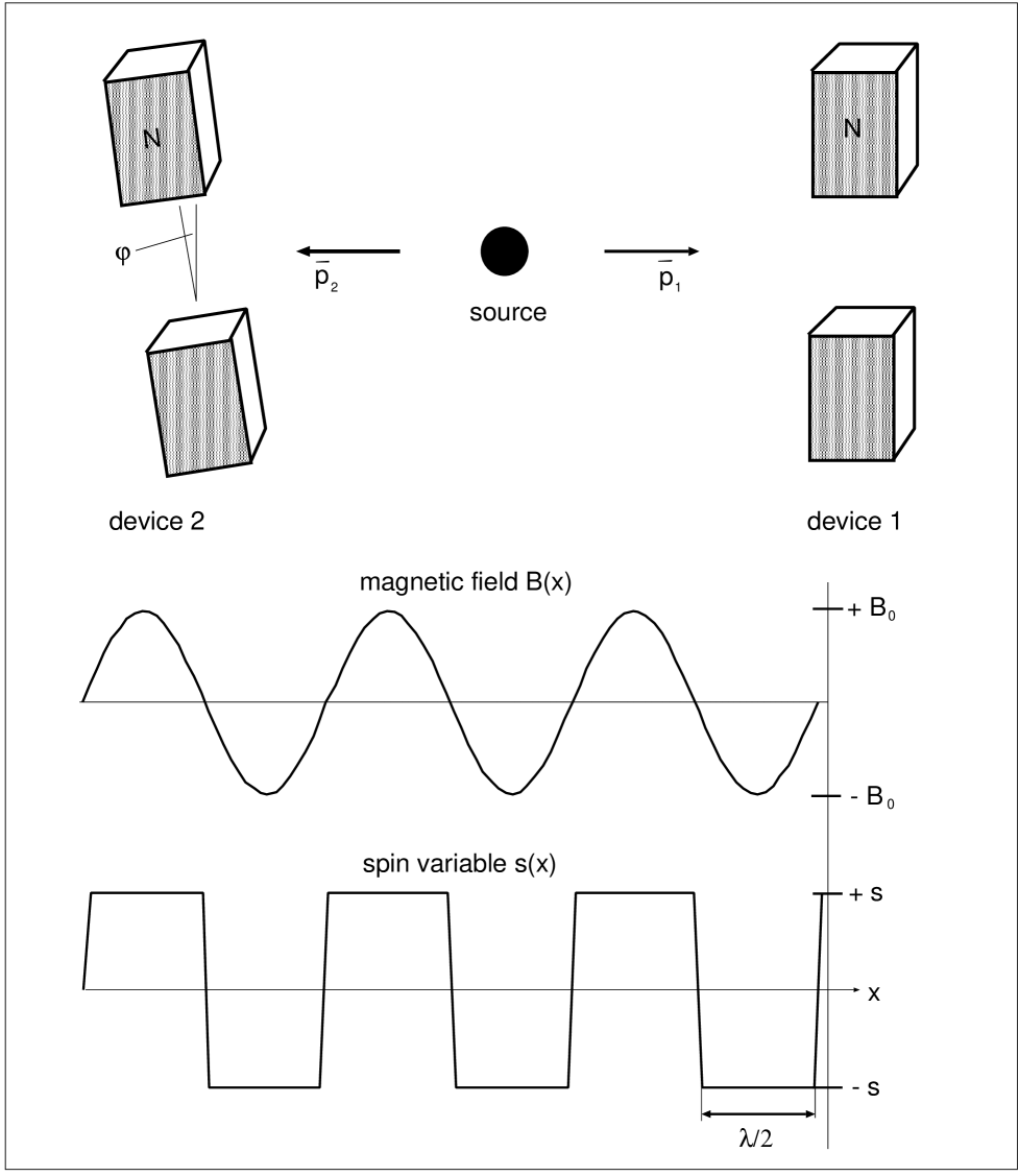
FIG. 1.: EPR measurement of spin variable. Two Stern–Gerlach devices (1,2) in different orientations used to determine the spin eigenvalues of the particles $\vec{p}_{1}$ and $\vec{p}_{2}$ from the source (top). The magnetic fields and spin variables depend on the position of measurement. Note that the spin variables are only constant in an interval shorter than $\lambda/2$ (bottom)

The second problem originates from the periodic features of the intrinsic magnetic field. Since the magnetic field vector is periodic with $\vec{B}=\vec{B}_{0}\cos(\vec{k}\vec{r}-\omega t)$, the spin variable cannot remain constant, but must oscillate from + 1 to - 1. This oscillation requires, that we define the exact moment of measurement to obtain any valid result on the state of either particle. If the photon path remains constant in measurements, this requirement is fulfilled, but if, like in Aspect’s measurements [35], the measuring apparatus has to be rotated to account for different angles of observation, the effect on measurements seems not easy to estimate. This problem therefore leads to a problem of experimental methods, which is hidden in the usual argumentation of quantum theory.

Provided, the problem can be accounted for, our next problem is more substantial. Since the spin variable oscillates, the measurement can only yield a definite result, if the variable is measured in the time–interval $t\leq\tau/2$, which requires, that the local resolution of the measuring apparatus is below $\triangle x\leq\lambda/2$. Now as demonstrated in the deduction of the uncertainty relations, this interval is equal to the lowest limit of local resolution in the framework of quantum theory. Thus we get the result, that a valid measurement of the spin–variable must have a local precision which is explicitly beyond the fundamental uncertainty in quantum theory. If, therefore, the measurements yield any correlation related to physical processes, then the fundamental axioms of quantum theory must be violated.

This result seems to turn the controversy about the EPR paradox into a new direction. It can be established, that the mathematical framework of quantum theory, describing the state of either particle by a superposition of the two possible states $\pm$ 1 is correct. But it can equally be established, that a significant correlation in spin–measurements is not, as Einstein suspected, a proof of hidden variables or a contradiction in terms of special relativity, but a proof of measurements below the fundamental level of uncertainty. If this sort of measurement is possible, then the uncertainty relations are violated.

• If EPR measurements are possible and yield a significant correlation for a pair of spin particles, then the uncertainty relations are violated.

M Compton scattering

In section III it was established, that electromagnetic radiation consists of two distinct intrinsic variables: (1) a longitudinal momentum, and (2) a transversal electromagnetic field, both variables depending on the frequency of radiation. In this section we found, that the change of energy density due to the adsorption of a photon result in motion of the absorbing electron, the energy increase given by:

$$\hbar\omega_{ph}=m_{el}u_{el}^{2}$$ (194)

If monochromatic x–rays therefore interact with free electrons , i.e. electrons with a velocity small compared to $\sqrt{\frac{\hbar\omega_{ph}}{m_{el}}}$, then the absorbing electrons should move in longitudinal direction with a velocity equal to:

$$u_{el}^{0}=\sqrt{\frac{\hbar\omega_{ph}}{m_{el}}}$$ (195)

If this electron is decelerated, then it will emit electromagnetic radiation with a frequency described by:

$$\frac{d\phi}{dt}=\frac{1}{V_{el}}h\nu^{2}$$ (196)

and, depending on the duration of the deceleration process, the radiation can possess arbitrarily low frequency. This primary emission therefore will not exhibit discrete frequency levels. But if secondary processes are considered, then the frequency change will depend on (1) the relative velocity between the source of radiation and the moving electron, and (2) the emission and absorption characteristics. Assuming, that the emission and absorption processes are symmetric in terms of duration, then the frequency of secondary emission will depend on the original frequency as well as the angle of emission. The model presented is therefore a simplification, and it cannot be excluded, that a precise and deterministic picture of the whole process will not yield a deviating result. But compared to the standard model in quantum theory [38], it is nevertheless an improvement, because it does not have to recur to mechanical concepts.

If the electron moves in longitudinal direction and with a velocity equal to $u_{el}^{0}$, the frequency $\nu_{S}$ of the source will be changed due to the electromagnetic Doppler effect. The secondary absorption process therefore has to account for a frequency $\nu_{S}^{\prime}$:

$$\nu_{S}^{\prime}=\nu_{S}\,\sqrt{\frac{1-\frac{u_{el}^{0}}{c}}{1+\frac{u_{el}^{0}}{c}}}\approx\nu_{S}\left(1-\frac{u_{el}^{0}}{c}\right)$$ (197)

An observer moving with the velocity $u_{el}^{0}$ of the electron will therefore measure changed frequencies and wavelengths of secondary emission. The wavelength $\lambda_{S}^{\prime}$ will be:

$$\lambda_{S}^{\prime}=\lambda_{S}\left(1+\frac{h}{mc}\frac{1}{\lambda_{S}}\right)=\lambda_{S}+\frac{h}{mc}$$ (198)

The second term, the shift of wavelength due to longitudinal motion of the electron relative to the source of radiation, is the Compton wavelength of an electron [39]. It is the general shift of wavelength for every electromagnetic field, and an expression of longitudinal motion.

$$\triangle\lambda\left(u_{el}^{0}\right)=\lambda_{C}=\frac{h}{mc}=\mbox{constant}$$ (199)

Additionally it has to be considered, that the reference frame of observation is the same as the reference frame of the original radiation, thus a second frequency shift depends on the angle of observation $\vartheta$. Measured from the direction of field propagation this additional shift will be:

$$u^{\prime}=u_{el}^{0}\cos{\vartheta}$$ (200)

And the overall shift of wavelength measured is therefore:

$$\triangle\lambda=\triangle\lambda\left(u_{el}^{0}\right)\left(1-\cos{\vartheta}\right)=\lambda_{C}\left(1-\cos{\vartheta}\right)$$ (201)

The result is equivalent to Compton’s measurements. Compton scattering, in our view, is therefore a result of (1) secondary absorption and emission processes, and of (2) successive Doppler shifts due to longitudinal motion of the emitting electrons. That classical electrodynamics does not provide a theoretical model for Compton scattering, can be understood as a consequence of neglecting longitudinal and kinetic features of photons. Since electromagnetic radiation in electrodynamics is interpreted from transversal properties alone (which are periodic), a uniform longitudinal motion due to absorption processes is not within its theoretical limits.

The possibility to account for quantum effects with the modified and still continuous model of electrons is strongly supporting, in our view, the validity of the unification of electrodynamics and quantum theory by formalizing the intrinsic features of particles.

V Conclusion

As it turns out, retrospectively, the theory of material waves removes the two fundamental problems, which made a physical interpretation (as opposed to the probability–interpretation [11]) of intrinsic wave properties impossible. (1) The contradiction between phase velocity and mechanical velocity of a particle wave is removed by the discovery of intrinsic potentials. (2) The problem of intrinsic Coulomb interactions is removed, because electrostatic interactions can be referred to an exchange of photons. A particle in uniform motion is therefore stable.

To exhibit the full range of logical and physical implications of the theory developed, we repeat the essential results of this essay on material waves, displayed throughout the preceding sections of this paper:

1. The interpretation of particles as physical waves allows the conclusion, that quantum theory cannot be, in a logical sense, a complete theoretical description of micro physical systems.

2. Because quantum theory neglects intrinsic characteristics of particle motion, the Schrödinger equation is generally not precise by a value described by Heisenberg’s uncertainty relations.

3. Electrodynamics and wave mechanics are theoretical concepts based on the same physical phenomena, the intrinsic features of moving particles.

4. The wave equations of intrinsic particle structures are Lorentz invariant only for an integral evaluation of energy. The total intrinsic potentials increase for every transformation into a moving frame of reference.

5. If intrinsic features of particles and their interactions are considered, quantization has to be interpreted as a result of energy transfer processes and their specific properties.

6. The elementary quantum of electron charge derives from energy transfer rates in electrostatic interactions, which are an expression of the interaction process accomplished by photons.

7. On the basis of electron–photon interactions Planck’s constant in material wave theory only applies to interactions and transfer processes. A justification of discrete frequencies, mass or charge values from the viewpoint of allowed states cannot be given. The result indicates, that the formalism of quantum theory lacks justification if it refers discrete energy levels to isolated particles.

8. The interpretation of electrostatic interactions as an exchange of photons, proper to material wave theory, has the consequence, that (1) the properties of single charges can only be referred to interactions with the environment, (2) photons can only be interpreted as particles if two identical charges interact, and (3) electrostatic potentials depend on the possibility of photon exchanges.

9. If EPR measurements are possible and yield a significant correlation for a pair of spin particles, then the uncertainty relations are violated.

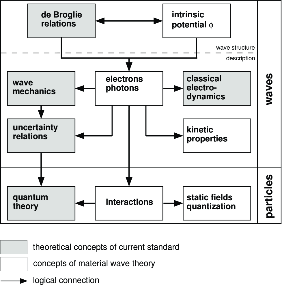
FIG. 2.: Logical structure of micro physics according to material wave theory. Classical electrodynamics and wave mechanics describe intrinsic features of particles, quantization arises from interactions.

The theoretical framework thus provides definite answers to the EPR paradox by rejecting the Copenhagen interpretation of quantum theory [9], because (1) quantum theory is not a complete account of micro physical systems, since the wave function possesses physical significance, and (2) the theory is logically inconsistent, since it is applicable only to interaction processes, while its mathematical formulation suggests the results to derive from properties of individual particles. Concerning Renninger’s objections on the quality of photons derived from thought experiments [31], it provides a model of photons where (1) the energy is homogeneously distributed over the whole region of electromagnetic fields, (2) the kinetic features of photons derive from a longitudinal component not accounted for in electrodynamics, and (3) the energy transfer in interactions applies for every single point of a given region, which yields the quantum effect of interaction.

VI Discussion

A General

It is difficult to estimate either the impact or the subsequent changes due to a concept, which completely deviates from the mainstream of current physics. The aim of establishing and, to a limited extent, interpreting a physical reality by an alternative framework was to provide a means, by which experimental results can be seen from at least two different points of view. The fundamental idea, it seems, is not very different from the conceptions of Einstein, Schrödinger, Bohm, or de Broglie (see the introduction), but the disregard of well established interpretations is considerably higher.

This was not, initially, intended. It only turned out, that a theoretical concept limited to only minor changes will neither provide a scientifically satisfying solution – since it still is based on some have to believe – nor does it really offer any new insight into micro physical processes. It was not intended to recover all the results of current quantum physics, not least, because it would surely require many lifetimes to succeed. But it was intended, and, so I think, accomplished rather successfully, to extend the theoretical framework of micro physics beyond the uncertainty relations and the we cannot know of quantum theory. Whether the result presented it the best possible way out of the dilemma arising from a physics of quantities – mechanics – confronted with a world of intensities – electrodynamics – cannot be currently estimated. To estimate the epistemological changes implied by the theoretical framework, Fig. 2 displays the logical structure of micro physics in material wave theory.

B Experimental

To estimate, whether the new theory contradicts any experimental evidence within its range of formalization, it has to be considered, that it provides a meta–theory combining the different frameworks of electrodynamics, quantum theory, and quantum electrodynamics in a single consistent framework.

From the viewpoint of electrodynamics, it will reproduce any result the current framework provides, because the basic relations are not changed, merely interpreted in terms of electron and photon propagation. Therefore an experiment, consistent with electrodynamics, will also be consistent with the new theory.

In quantum theory, the only statements additional to the original framework are beyond the level of experimental validity, defined by the uncertainty relations. Since quantum theory cannot, in principle, contain results beyond that level, every experiment within the framework of quantum theory must necessarily be reproduced. That applies to the results of wave mechanics, which yields the eigenvalues of physical processes, as well as to the results of operator calculations, if von Neumann’s proof of the equivalence of Schrödinger’s equation and the commutator relations is valid. The only result, which could in this respect disprove the theory, is the spreading of a wave packet: but as this experimental result was the reason, that a physical interpretation of wave functions had to be discarded, the theory also in this respect seems to stand on firm ground.

In quantum field theory, the same rule applies: the new theory only states, what is, in quantum theory, no part of a measurement result, therefore a contradiction cannot exist. If, on the other hand, results in quantum electrodynamics exist, which are not yet verified by the new theory, then it is rather a problem of further development, but not of a contradiction with existing measurements.

C Theoretical

Experimentally, the new theory cannot be disproved by existing measurements, because its statements at once verify the existing formulations and extend the framework of theoretical calculations. The same does not hold, though, for the verification of existing theoretical schemes of calculation by the new framework. Since the theory extends far beyond the level of current concepts, established theoretical results may well be subject to revision. The theory of material waves requires, that every valid solution of a microphysical problem can be referred to physical properties of particle waves. In cases, where the established theory provides a solution yielding, for example, correct eigenvalues but not wave functions which can be identified as physical waves, the result is, from this viewpoint, questionable. Essentially, this is not limiting nor diminishing the validity of current results, since it extends the framework of micro physics only to regions, which so far have remained unconsidered.

VII Outlook

From the five tasks defined in the introduction as our personal criterium for a promising new approach, three have been accomplished by this publication. But as quantum theory, historically, was invented due to the puzzling results in atomic physics, the whole concept as such would be useless without a theory of atoms compatible with the framework developed. This theory has partly been published already (see [19]), partly it is still in the making although the essential results have been derived. It will be the aim of the next paper published in the internet, to give a thorough and up to date account of a model of hydrogen atoms in terms of material waves.

REFERENCES

- [1] Schweber S. QED and the Men Who Made It, Princeton (1994)
- [2] Bohm D. Causality and Chance in Modern Physics, Princeton (1957)
- [3] de Broglie L. in his foreword to [2]
- [4] Dirac P.A.M. Eur. J. Phys. 5, 65 (1984)
- [5] Röseberg U. in Götschl J. (ed.) Erwin Schrödinger’s world view, Dordrecht (1992) p. 135
- [6] Feynman R. QED, Princeton (1988) p.9
- [7] Schrödinger, E. Ann. Physik 79, 361; 489 (1926)
- [8] Heisenberg W. “Remarks on the Origin of Uncertainty” in Price W. C. (ed.) The Uncertainty Principle and the Foundations of Quantum Mechanics, Wiley & Sons, New York (1977)
- [9] Bohr N. “Discussion with Einstein on Epistemological Problems in Atomic Physics”, in A. Einstein: Philosopher–Scientist, Schilpp P.A. (ed.), Harper and Row, New York (1959)
- [10] de Broglie L. Ann. Phys. 3, 22 (1925)
- [11] Born, M. Z. Physik 37, 863 (1926)
- [12] Einstein A., Rosen N., and Podolsky B. Phys. Rev. 47, 180 (1935)
- [13] Kwiat P., Weinfurter H., Herzog T., Zeilinger A., and Kasevich M.A. Phys. Rev. Lett. 74, 4763 (1995)
- [14] Renninger M. Zeitschr. f. Phys. 158, 417 (1960)
- [15] Bohm, D. Phys. Rev. 85, 166; 180 (1952)
- [16] Bell J.S. Physics 1, 195 (1964); see also his remarks on hidden variable theories in Rev. Mod. Phys. 38, 447 (1966)
- [17] Davisson C. and Germer L.H. Phys. Rev. 30, 705 (1927)
- [18] Hofer W. A. Internal energy of free particles: de Broglie waves in electrodynamics. Specs. Sci. Tech. 18, 157 (1995)
- [19] Hofer W. A. An inertial model of atoms: atomic spectra as a resonance problem. Specs. Sci. Tech., in print
- [20] Born M., Heisenberg W., and Jordan P. Z. Physik 35, 557 (1926)
- [21] Planck M. Ann. Physik 4, 553 (1901)
- [22] Heisenberg W. Z. Physik 43, 172 (1927)
- [23] Cohen–Tannoudji C., Diu B., and Laloe F. Quantum Mechanics, Wiley & Sons, New York (1977)
- [24] Einstein A. Ann. Physik 17, 891 (1905)
- [25] Sommerfeld A. Elektrodynamik, Akademische Verlagsgesellschaft, reprint Leipzig (1964)
- [26] Michelson, and Morley. Amer. J. Sci. 34, 333 (1887) ; Phil. Mag. 24, 449 (1887)
- [27] Jackson J. Classical Electrodynamics, Wiley & Sons, New York (1984)
- [28] Einstein A. Ann. Physik 17, 132 (1905)
- [29] Jordan P. Anschauliche Quantentheorie, Berlin (1936) p. 115
- [30] Heisenberg W. Die physikalischen Grundlagen der Quantentheorie, Leipzig (1941) p. 7 and 107
- [31] Renninger M. Z. Physik 136, 251 (1953)
- [32] A. Einstein. Ann. Physik 20, 627 (1906)
- [33] UIPAP document UIP 20. Physica A 93, 1 (1978)
- [34] Bohm D. Quantum Mechanics, Prentice–Hall, Eaglewood Cliffs (1951)
- [35] Aspect A. Trois tests experimenteaux des inegalites de Bell par mesure de correlation de polarisation de photons, Ph. D. thesis, Universite de Paris–Sud, Centre d’Orsay (1983)
- [36] Thompson C. H. Found. Phys. Lett. 9, 357 (1996)
- [37] Uhlenbeck G. E. and Goudsmit S. A. Naturwiss. 13, 953 (1925); and Nature 117, 264 (1925)
- [38] Debye, P. Phys. Zeitschr. 24, 161 (1923)
- [39] Compton, A. H. Phys. Rev. 22, 409 (1923)