A Framework for Quantum Search Heuristics

Abstract

A quantum algorithm for combinatorial search is presented that provides a simple framework for utilizing search heuristics. The algorithm is evaluated in a new case that is an unstructured version of the graph coloring problem. It performs significantly better than the direct use of quantum parallelism, on average, in cases corresponding to previously identified “phase transitions” in search difficulty. The conditions underlying this improvement are described. Much of the algorithm is independent of particular problem instances, making it suitable for implementation as a special purpose device.

1 Introduction

Quantum computers [1, 2, 7, 8, 10, 17, 9] use quantum parallelism, i.e., the ability to operate simultaneously on a superposition of many classical states, and interference among different computational paths. A measurement on a superposition gives a definite result, with probabilities determined by the amplitudes of the superposition. A successful algorithm is one that uses these capabilities to arrange for a large probability of a desired result, e.g., a solution to a search problem.

However, there are two major difficulties with quantum computers. First, they are difficult to implement [16]. Second, the physical restriction to unitary linear operations makes quantum computers difficult program effectively. An encouraging development with respect to the design of algorithms is a method for efficiently factoring integers [23], a problem that appears to be intractable for classical computers. Since this relies on specific properties of the factoring problem, the extent to which effective quantum algorithms can be developed for general combinatorial search remains an open question.

To help address this question empirically, it would be useful to have a simple framework for exploring the use of search heuristics with quantum algorithms. Specifically, such a framework should allow a variety of heuristic search methods to be programmed while automatically preserving a number of desirable properties that simplify potential hardware implementations. This could serve to bridge the gap between discussions of hardware, with the focus usually on bit-level operations, and abstract theoretical discussions, with the focus on Turing machines and general unitary operations.

There are a number of desirable properties such a framework should provide for a general quantum search algorithm. First, the number of computational steps required should be determined a priori. This avoids the question of when to make the final measurement, and could limit the difficulties of decoherence compared to running a program where the number of steps required can vary greatly from one problem instance to the next. Second, it is useful if much of the complexity of the algorithm can be made independent of the details of individual instances. This can facilitate implemention with a special purpose search device. Third, the framework should easily allow applying heuristics that incorporate additional knowledge about the structure of particular search problems, in a manner analogous to the heuristics used to dramatically improve many classical search strategies.

Another property is given by recent studies of the nature of classes of combinatorial search problems and relates to how methods are evaluated. Most theoretical analyses of search algorithms focus on worst case behavior. However, in practice it is often more important to examine the behavior of algorithms for typical or average search problems. Thus even if quantum computers are not applicable to all combinatorial search problems, they may still be useful for many instances encountered in practice. This is an important distinction since typical instances of search problems are often much easier to solve than is suggested by worst case analyses, though even typical costs often grow exponentially on classical machines.

In fact, the hard instances are not only rare but also concentrated near abrupt transitions in problem behavior analogous to physical phase transitions [5, 13, 12]. This result applies to many classical search methods that use problem structure to guide choices, but not to generate-and-test, where possible solutions are examined sequentially. Similarly, the most direct use of quantum parallelism for search, in which all states are simultaneously checked for consistency and then a measurement made, is equivalent to generate-and-test and does not exhibit the transition behavior. This limitation may apply to any search algorithm that uses quantum parallelism without also using interference [4]. Thus a check on whether a quantum algorithm is fully exploiting problem structure, through interference among different computational paths, is whether it exhibits the transition behavior. This is another useful property to incorporate in a general search framework.

In this paper, we briefly describe a previously proposed general search mechanism and discuss how it meets these criteria as well as some implementation issues. To examine its generality, its behavior is then evaluated empirically for a new problem ensemble, motivated by the NP-complete graph coloring problem. As with other previously studied problems, this shows a significant enhancement of probably to obtain a solution compared to the direct use of quantum parallelism and the transition behavior. We give a more detailed look at the underlying basis for this improvement to see how heuristics might be usefully applied. Finally, some open issues are presented.

2 A Quantum Search

Combinatorial search can be viewed as finding, from among $N$ given items, a set of size $L$ satisfying specified constraints. Such a set is a solution to the problem. The constraints, in turn, can be specified by nogoods, sets of items that are inconsistent. Because the supersets of a nogood are also nogood, sets of items can be viewed as forming a lattice structure consisting of levels from 0 to $N$. Level $i$ in this lattice contains all sets of size $i$, and these are linked to their supersets at the next level and subsets at the previous one. This lattice, describing the consistency relationships among sets, is the deep structure of the combinatorial search problem [24]. This structure for $N=4$ is shown in Fig. 1. Solutions are found among the sets at level $L$. Notationally, we denote the size of a set $s$ by $|s|$.

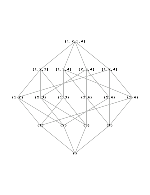
Figure 1: Structure of the set lattice for a problem with four items. The subsets of ${\left\{1,2,3,4\right\}}$ are grouped into levels by size and lines drawn between each set and its immediate supersets and subsets. The bottom of the lattice, level 0, represents the single set of size zero, the four points at level 1 represent the four singleton subsets, etc.

This abstract description of search is less commonly used than other representations, which are more compact and efficient for classical search algorithms. It is introduced here as a useful basis for quantum searches and because it applies to many search problems. These include constraint satisfaction problems (CSPs) [18] such as graph coloring and satisfiability. For example, in coloring an $n$-node graph with $c$ colors an item is a pair ${\left(\nu,\kappa\right)}$ consisting of a node $\nu$ in the graph and a color $\kappa$ for it. Thus there are $N=nc$ items and a solution consists of $L=n$ such items that give a unique color to each node and distinct colors to each pair of nodes in the graph that are linked by an edge. Each edge is a constraint which gives $c$ nogoods, each consisting of a pair of items with the same color for both of the nodes linked by that edge. This search problem is known to be NP-complete for a fixed $c$ (at least equal to 3) as $n$ grows. From this example, we see that an interesting scaling regime for combinatorial search is for the nogoods of the constraints to have a fixed, small size (e.g., at level 2 in the lattice for graph coloring) while the number of items and the size of solutions grows linearly with problem size.

There are many paths through the lattice from small sets to the larger sets at the solution level. For example, if $N=4$ and $L=2$, there are two paths from level zero to each set at level 2 in the lattice. E.g., the set ${\left\{1,2\right\}}$ is obtained via the paths $\emptyset{\rightarrow}{\left\{1\right\}}{\rightarrow}{\left\{1,2\right\}}$ and $\emptyset{\rightarrow}{\left\{2\right\}}{\rightarrow}{\left\{1,2\right\}}$. These multiple paths can be used to create interference with a quantum computer operating on a superposition of sets. One way to do this uses the fact that for search problems in NP it is relatively easy to test whether a particular set satisfies the given constraints. Thus, we can adjust the phase of the amplitudes along each path based on whether the associated set is consistent with the constraints. These phase adjustments attempt to create destructive interference among paths leading to nonsolutions and constructive interference for solutions. To the extent this is successful, amplitude will be concentrated into solution states, giving a relatively high probability to obtain a solution in the final measurement. A quantum computer with $N$ bits can simultaneously operate on superpositions of all $2^{N}$ subsets of ${\left\{1,\ldots,N\right\}}$. Thus we can start with a superposition consisting of small subsets, and move up one level at a time to the solution level, exploring all possible paths

Following this general concept, there are many possible mappings among these sets. A particularly simple method is to divide the mapping into two parts. The first is problem-independent and moves amplitude from sets of a given size to the next larger size. The second is an adjustment to the phases of the sets at the new level. A simple choice for the phase adjustment process is to change the sign of the amplitude of each inconsistent set encountered. While this is not always the optimal phase policy, it has the advantage of being easily computable since it operates independently on each set and, as shown below, is quite effective.

The mapping from one level to the next is a more complex quantum operation as it involves mixing the amplitude from different states. On the other hand, this mapping is independent of the details of individual problem instances which could simplify its implementation as a special purpose search device instead of a program operating on a universal quantum computer. It is this part of the algorithm that gives rise to interference effects by mixing the contribution from different paths through the lattice. The operation used here is motivated by breadth-first classical search where each consistent set is extended to each possible superset at the next level. Such a mapping is not unitary, though it is nearly so. Thus a simple choice for the quantum mapping is to use that unitary operator that is closest [11] to the mapping of sets equally to their supersets. The resulting matrix elements have a simple structure, depending only on the size of the intersection of the corresponding sets [14].

2.1 The Search Method

The search algorithm starts by evenly dividing amplitude among the goods at a low level of the lattice. For problems such as graph coloring where the constraint nogoods involve only two items at a time, a reasonable choice is to start at level 2, where the number of sets is proportional to $N^{2}$. Then for each level from 2 to $L-1$, we adjust the phases of the states depending on whether they are consistent and map to the next level. Let $\psi^{{\left(j\right)}}_{s}$ be the amplitude of the set $s$ at level $j$ after completing step $j-2$ of the algorithm. The initial condition is $\psi^{{\left(2\right)}}_{s}=1/\sqrt{N_{\rm goods}}$ if the set $s$ at level 2 is good, i.e., consistent with the constraints, and otherwise $\psi^{{\left(2\right)}}_{s}=0$. Here $N_{\rm goods}$ is the number of consistent sets at level 2.

Each step of the algorithm moves up one level giving

$${\psi^{{\left(j+1\right)}}_{r}=\sum_{k=0}^{j}a^{{\left(j\right)}}_{k}\sum_{{\left|r\cap s\right|}=k}\rho_{s}\psi^{{\left(j\right)}}_{s}}$$

(1)

where $a^{{\left(j\right)}}_{k}$ is the problem-independent matrix element mapping from sets $s$ of size $j$ to those $r$ of size $j+1$ that have $k$ elements in common with $s$, $\rho_{s}$ is the phase assigned to the set $s$ after testing whether it is nogood, and the inner sum is over all sets $s$ of size $j$ that have $k$ items in common with $r$. That is, $\rho_{s}=1$ when $s$ is a good, and otherwise $\rho_{s}=-1$.

After $L-2$ steps we measure the state, obtaining a single set. This set will be a solution with probability

$${P_{\rm soln}=\sum_{s}p{\left(s\right)}}$$

(2)

with the sum over solution sets and $p{\left(s\right)}={\left|\psi^{{\left(L\right)}}_{s}\right|}^{2}$ is the probability to obtain the set $s$ with the measurement of the final state.

2.2 Classical Simulation

The study of the average or typical behavior of search heuristics relies primarily on empirical evaluation. This is because the complicated conditional dependencies in search choices made by the heuristic often preclude a simple theoretical analysis, although phenomenological theories can give an approximate description of some generic behaviors [13, 15, 20]. Thus as a practical matter, the search framework described here should allow for empirical evaluation of various heuristic methods on existing classical computers.

Unfortunately, the exponential slowdown and growth in memory required for such a simulation severely limits the feasible size of the search problems. To see this, note that (1) consists of a matrix multiplication on a vector of size $N_{j}={N\choose j}$, equal to the number of sets at level $j$ of the lattice, to produce a new vector of size $N_{j+1}$. A direct evaluation of this mapping requires of order $N_{j}N_{j+1}$ multiplications. To reach the solution level at $L=O{\left(N\right)}$ requires mapping at relatively high levels in the lattice where $j=\eta N$ with $\eta$ constant. In this case $\ln N_{j}\sim Nh{\left(\eta\right)}$ where $h{\left(\eta\right)}=-\eta\ln\eta-{\left(1-\eta\right)}\ln{\left(1-\eta\right)}$, so the classical computation cost scales according to $e^{2h{\left(\eta\right)}N}$, which is $2^{2N}$ when $\eta=1/2$.

The cost of the classical simulation can be reduced substantially (though still growing exponentially) by exploiting the map’s simple structure with a recursive evaluation. This is done by expanding the map in (1) to include all $2^{N}$ sets of $N$ items and then writing (1) as

$${\psi^{{\left(j+1\right)}}_{r}}$$

(3)

where $x_{s}\equiv\rho_{s}\psi^{{\left(j\right)}}_{s}$ is the original state modified by the choice of phases for each set, which is nonzero only for sets of size $j$.

From the definition of $V_{rjk}$, it follows that

$${\sum_{{r^{\prime}\subset r}\atop{{\left|r^{\prime}\right|}={\left|r\right|}-1}}V_{r^{\prime}jk}={\left({\left|r\right|}-k\right)}V_{rjk}+{\left(k+1\right)}V_{rj,k+1}}$$

(4)

The sum in this expression is only over the ${\left|r\right|}$ subsets of $r$ of size ${\left|r\right|}-1$ and so can be rapidly computed for a given set $r$. From this relation, $V_{rj,k+1}$ can be determined easily given $V_{rjk}$ and the values for the subsets of $r$ with one element removed. Hence, from the values for $V_{rj0}$ we can readily determine the $V_{rjk}$ for $k>0$ iteratively starting from $r=\emptyset$ at the bottom of the lattice and moving up a level at a time until the values at level $j+1$ are determined.

To evaluate $V_{rj0}$ define the matrix $A$, of size $2^{N}\times 2^{N}$, with elements $A_{rs}$ equal to zero if ${\left|r\cap s\right|}>0$, i.e., the sets have an element in common, and one otherwise. Let $y_{r}=\sum_{s}A_{rs}x_{s}$. Because $x_{s}$ is zero unless the set $s$ is of size $j$, we have

$$V_{rj0}=y_{r}$$ (5)

The product $A{\bf x}$ can be computed recursively. To see this consider the sets ordered by the value of the integer with corresponding binary representation, e.g., the sets without item $N$ come before those with $N$. For example, the sets for $N=3$ are ordered as $\{\}$, $\{1\}$, $\{2\}$, $\{1,2\}$, $\{3\}$, $\{1,3\}$, $\{2,3\}$ and $\{1,2,3\}$. In this ordering, the matrix $A$ has the recursive decomposition

$${A={\left(\matrix{A^{\prime}&A^{\prime}\cr A^{\prime}&0\cr}\right)}}$$

(6)

where $A^{\prime}$ is the same matrix but defined on subsets of ${\left\{1,\ldots,N-1\right\}}$ and 0 is the matrix all of whose entries equal zero. We can then compute

$${A{\bf x}={\left({A^{\prime}{\bf x^{{\left(1\right)}}}+A^{\prime}{\bf x^{{\left(2\right)}}}}\atop{A^{\prime}{\bf x^{{\left(1\right)}}}}\right)}}$$

(7)

where ${\bf x^{{\left(1\right)}}}$ and ${\bf x^{{\left(2\right)}}}$ denote, respectively, the first and second halves of the vector x (i.e., corresponding to sets without $N$ and with $N$ respectively). Thus the cost to compute $A{\bf x}$ is $C{\left(N\right)}=2C{\left(N-1\right)}+O{\left(2^{N}\right)}$ resulting in an overall cost of order $N2^{N}$. While still exponential, this improves substantially on the cost for the direct evaluation at high levels of the lattice.

This calculation can be improved further in two ways. First, when computing y recursively store only the components for sets of size $j+1$ or smaller. The values for larger sets are never used. Second, there is no need to explicitly compute and store the $V_{rjk}$ values individually. This is because we are only interested in a particular linear combination of these values in (1) for sets $r$ of size $j+1$. Using (4) this can be determined from a linear combination of values for sets of size $j$, and so on down to the bottom of the lattice. The net result of this process means the map of (1) becomes a product of matrices, one for each step up the lattice, which in turn multiplies the vector $A{\bf x}$ computed recursively as described above.

The basic components of this computation, a recursive matrix combined with a simple relation to build up the required linear combinations, are not unique. Other possibilities are useful to keep in mind as they may differ in their sensitivity to errors and also suggest a variety of quantum implementations. For instance, instead of the matrix $A$ used above, defining $B_{rs}={\left(-1\right)}^{{\left|r\cap s\right|}}$ gives

$${B={\left(\matrix{B^{\prime}&B^{\prime}\cr B^{\prime}&-B^{\prime}\cr}\right)}}$$

(8)

which is unitary when normalized by dividing each element by $2^{N/2}$. Thus ${\bf z}=B{\bf x}$ also has a simple recursive evaluation. This can be used as the basis for computing the $V_{rjk}$ by noting that (5) can be replaced with $\sum_{k=0}^{j}{\left(-1\right)}^{k}V_{rjk}=z_{r}$. Furthermore, instead of building up the values from subsets with (4), an alternate relation is

$${\sum_{r^{\prime}}B_{rr^{\prime}}V_{r^{\prime}jk}=\sum_{l=0}^{j}V_{rjl}n_{lk{\left|r\right|}j}}$$

(9)

where the sum over $r^{\prime}$ includes all sets and $n_{lk\rho\sigma}=\sum_{m=0}^{\rho}{\left(-1\right)}^{m}n_{lk\rho\sigma;m}$ with

$${n_{lk\rho\sigma;m}=2^{N-\rho-\sigma+l}\sum_{x=0}^{l}{{\rho-l}\choose{m-x}}{{l}\choose{x}}{{\sigma-l}\choose{k-x}}}$$

(10)

counting the number of sets $r^{\prime}$ with overlap $k$ with $s$ and $m$ with $r$, given that $s$ and $r$ have overlap $l$ and sizes $\sigma$ and $\rho$ respectively. These relations involve somewhat more computational operations on a classical machine than the method described above. However, by avoiding use of the nonunitary mapping between each set and its subsets, it may provide a method whereby quantum computers could exploit the simple structure of the mapping.

3 Quantum Search Behavior

The behavior of this search algorithm was examined through a classical simulation. While these results are limited to small search problems, they nevertheless give an indication of how this algorithm can dramatically increase the probability to find solutions compared to the direct use of quantum parallelism. As a check on the numerical errors, the norm in the final state was 1 to within $10^{-10}$.

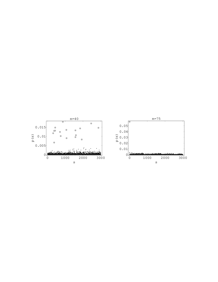
Figure 2: Probability in sets at the solution level for two instances of unstructured problems with $N=15$. On the left, the problem has $m=40$, with 17 solutions and $P_{\rm soln}=0.21$, on the right, $m=75$, with a single solution and $P_{\rm soln}=0.057$. The solutions are drawn as large gray points. The remaining sets are small black points.

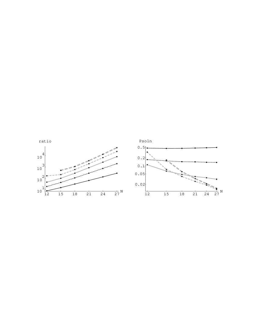
Figure 3: Scaling of the algorithm. The left plot shows the ratio of probability to find a solution, $P_{\rm soln}$, with the algorithm to that from random selection from among the solution level sets, for $L=N/3$ with prespecified solution for $\beta=m/N$ of 2 (solid), 3 (dashed), 4 (gray), 5 (dashed gray) and 6 (thick dashed gray). This is shown on a log-scale. The right plot shows the scaling of $P_{\rm soln}$ on a log-log plot. Each point is the average of 1000 problem instances (except only 100 were used for $N=27$). The points include error bars indicating the standard error of estimates of the mean, which in most cases are smaller than the size of the plotted points.

As an example of the average behavior we consider a simple class of unstructured problems corresponding to graph coloring with 3 colors. As described above, a graph with $n$ nodes has $N=3n$ variable-value pairs, and solutions consist of sets of $L=n=N/3$ of these items. The constraints in a graph coloring problem involve two items at a time. Thus to randomly generate an unstructured version of such a problem, we select $m$ distinct sets, each with two items, to be the nogoods specified by the constraints. There are ${N\choose 2}$ such sets to choose from. This random selection of problems ignores the detailed structure of the constraints for graph coloring, but gives a wider range of possible $m$ values for the small problems considered here.

Since the quantum algorithm is incomplete, i.e., it can find a solution but never determine that no solution exists, we consider only problems with a solution. Soluble problems are rare when there are many nogoods, so for simplicity we use a prespecified solution, i.e., before selecting the nogoods, a particular set of size $L$ is selected to be a solution. Then, the selection of $m$ nogoods is only from among those that are not subsets of this specified solution. This guarantees the problem has at least one solution. Qualitatively similar results are obtained by full random selection and then testing, via a complete classical search, that the problem has a solution.

Fig. 2 shows how the algorithm enhances the probability of finding a solution for two instances: one with few constraints and the other with many constraints. The sets are ordered according to the integer whose binary representation corresponds to including the items in the set [21]. In this case there are ${15\choose 5}=3003$ sets at the solution level, so a random selection would give a probability of about 0.0003 to each set, much less than given to solutions by this algorithm. Thus the various contributions to nonsolutions tend to cancel out among the many paths through the lattice.

3.1 Scaling

Fig. 2 shows the improvement over generate-and-test for two cases, but how well does the algorithm do over the ensemble of problems, and how does this behavior scale with increasing problem size? An appropriate choice of the scaling and method of generating problem instances is necessary for a study of average behavior so as to include a significant number of hard instances. In this respect, an interesting scaling regime is when the number of nogoods at level 2 grows linearly with the size of the problem $N$, so we define $\beta\equiv m/N$. This corresponds to graph coloring where the number of edges is proportional to the number of nodes, which has a high concentration of hard search cases [5].

For these problems, two views of the scaling behavior are shown in Fig. 3. First, the linear growth on the log plot indicates this algorithm improves exponentially compared to the direct use of quantum parallelism. This is another indication of the effectiveness of this simple algorithm at concentrating amplitude into solutions. The second plot in the figure shows the overall probability to find a solution, on a log-log plot, where linear behavior corresponds to a power law. Here the problem sizes feasible for classical simulation are too small to see the asymptotic behavior clearly. Nevertheless, it appears to do quite well for problems with few constraints. And for the remaining cases, a fit to a power law is closer than an exponential. We conclude that this algorithm improves greatly on direct use of quantum parallelism, but it is unclear whether that is enough to give polynomial rather than exponential decrease of $P_{\rm soln}$, on average.

3.2 Phase Transition

Another indication of the usefulness of this quantum search algorithm is its behavior as the number of constraints are changed for problems of a given size. This is shown in Fig. 4. Significantly, the figure shows this search algorithm also exhibits the transition behavior that was described above as occurring for many classical searches [5], i.e., hard instances are concentrated near a change from underconstrained to overconstrained problems. Furthermore, the expected number of trials needed to find a solution is essentially constant when there are relatively few constraints. This appears to correspond to a second phase transition predicted to occur among weakly constrained problems [13]. Thus the algorithm is using interference of paths to exploit problem structure in the same manner as sophisticated classical search methods are observed to do.

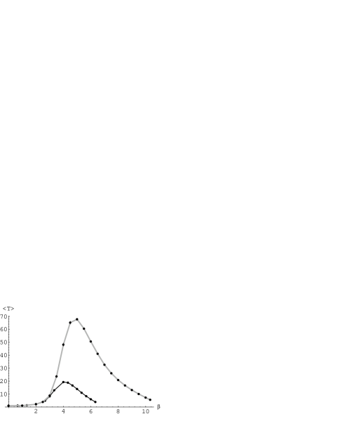
Figure 4: Average number of trials to find a solution, ${\left\langle T\right\rangle}=1/P_{\rm soln}$ as a function of $\beta$ for $N=15$ and 24 (black and gray curves, respectively). Each point is the average of 1000 problem instances, and includes error bars indicating the standard error of the mean, which in most cases are smaller than the size of the points.

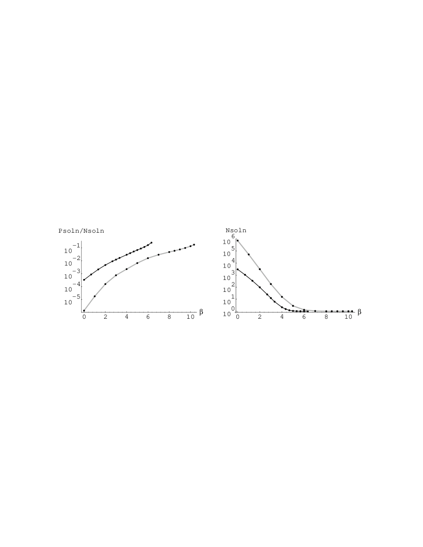
Figure 5: The underlying trade-off giving the transition behavior for $N=15$ and 24 (black and gray curves, respectively). The left plot shows the average probability in each solution set, $P_{\rm soln}/N_{\rm soln}$, as a function of $\beta$. The right plot shows the average number of solutions $N_{\rm soln}$. Both plots are on a log scale. Each point is the average of 1000 problem instances, and includes error bars indicating the standard error of the mean, which are smaller than the size of the points.

This can be understood from Fig. 5, showing how the average value for $p{\left(s\right)}$ among solutions compares with the expected number of solutions $N_{\rm soln}$ for problems with differing numbers of constraints. The average probability per solution grows as constraints are added. Thus the simple method of inverting phases at each nogood becomes increasingly effective as more nogoods are added to the lattice. However, this growth is initially overwhelmed by the even faster decrease in the number of solutions, leading to a smaller chance to find a solution, i.e., harder problems. Eventually the number of solutions stops decreasing so rapidly because the constraints have already eliminated most solutions. At this point the continued improvement in concentration of amplitude into the remaining solutions dominates, so problems get easier. Using such a figure to display the concentration of amplitude into solutions can also be useful for viewing the behavior of different choices for the phases introduced at inconsistent sets in the lattice, perhaps in conjunction with the use of heuristics.

Similar behaviors have also been seen for other problem ensembles [14]. These include cases corresponding to binary CSPs with two values per variable, i.e., $L=N/2$, and the NP-complete 3SAT problem where the constraint nogoods are sets of size 3. For these types of problems, slightly different ensembles can be produced through changes in the way problem instances are generated. Although all these empirical observations are limited to small problem sizes, they do suggest the search method applies generally to a wide range of problem ensembles.

4 Conclusion

The lattice structure provides a general framework for applying quantum computers to search problems. It has the advantage of an a priori specification of the required computational steps and provides many opportunities for using interference among the paths through the lattice to each set at the solution level. While unlikely to work as well as special purpose algorithms for particular search problems, this framework may provide a basis for high performance search, on average, over a wide range of problem types.

One important feature of this search framework is the ability to incorporate additional knowledge about the particular problem structure or other search heuristics. This is readily included as a modification to the choice of phases because any such choice is guaranteed to be a unitary operation and can operate independently on each state. Changes to the mapping from one level to the next are more complicated due to the requirement to maintain unitarity (as well as computational simplicity). Another way to incorporate heuristics is by changing the initial conditions. In the method reported here, initially all amplitude is in small consistent sets. The hope then is that this concentration in consistent sets is maintained as amplitude is moved up through the lattice. Instead, one could start with amplitude spread among all sets and try to arrange for it to be concentrated into consistent sets only by the time it reaches the solution level. In some cases, this is observed to increase the concentration into solutions.

As a possible extension to this algorithm, it would be interesting to see whether the nonsolution sets with relatively high probability could be useful also, e.g., as starting points for a local repair type of search [19]. If so, the benefits of this algorithm would be greater than indicated by its direct ability to produce solution sets. This may also suggest similar algorithms for the related optimization problems where the task is to find the best solution according to some metric, not just one consistent with the problem constraints.

There remain a number of important questions. First is the issue of implementation of the map from one level of the lattice to the next in terms of more elementary operations that are physically realizable. This could lead to the construction of special purpose search devices for the set manipulations used in the problem-independent mapping between levels of the lattice. Second, how are the results degraded by errors and decoherence, the major difficulties for the construction of quantum computers [16]? While there are some quantum approaches to error control [3, 22] and studies of decoherence in the context of factoring [6] it remains to be seen how these problems affect the framework presented here. Third, it would be useful to have a theory for asymptotic behavior for large $N$, even if only approximately in the spirit of mean-field theories of physics. This would give a better indication of the scaling behavior than the classical simulations, necessarily limited to small cases, and may also suggest better phase choices. Considering these questions may suggest simple modifications to the quantum map to improve its robustness and scaling. There thus remain many options to explore for using the deep structure of combinatorial search problems as the basis for general quantum search methods.

References

- [1] Benioff, P. (1982), “Quantum Mechanical Hamiltonian Models of Turing Machines”, J. Stat. Phys. 29, 515–546.
- [2] Bernstein, Ethan, and Umesh Vazirani (1993), “Quantum Complexity Theory”, In Proc. 25th ACM Symp. on Theory of Computation, 11–20.
- [3] Berthiaume, Andre, David Deutsch, and Richard Jozsa (1994), “The Stabilization of Quantum Computations”, In Proc. of the Workshop on Physics and Computation (PhysComp94), 60–62, Los Alamitos, CA, IEEE Press.
- [4] Cerny, Vladimir (1993), “Quantum Computers and Intractable (NP-complete) Computing Problems”, Physical Review A 48, 116–119.
- [5] Cheeseman, Peter, Bob Kanefsky, and William M. Taylor (1992), “Computational Complexity and Phase Transitions”, In Proc. of the Workshop on Physics and Computation (PhysComp92), 63–68, Los Alamitos, CA, IEEE Computer Society Press.
- [6] Chuang, I. L., R. Laflamme, P. W. Shor, and W. H. Zurek (1995), “Quantum Computers, Factoring and Decoherence”, Science 270, 1633–1635.
- [7] Deutsch, D. (1985), “Quantum Theory, the Church-Turing Principle and the Universal Quantum Computer”, Proc. R. Soc. London A 400, 97–117.
- [8] Deutsch, D. (1989), “Quantum Computational Networks”, Proc. R. Soc. Lond. A425, 73–90.
- [9] DiVincenzo, David P. (1995), “Quantum Computation”, Science 270, 255–261.
- [10] Feynman, R. P. (1986), “Quantum Mechanical Computers”, Foundations of Physics 16, 507–531.
- [11] Golub, G. H., and C. F. Van Loan (1983), Matrix Computations, John Hopkins University Press, Baltimore, MD.
- [12] Hogg, Tad (1994), “Phase Transitions in Constraint Satisfaction Search”, A World Wide Web page with URL ftp://parcftp.xerox.com/pub/dynamics/constraints.html.
- [13] Hogg, Tad (1994), “Statistical Mechanics of Combinatorial Search”, In Proc. of the Workshop on Physics and Computation (PhysComp94), 196–202, Los Alamitos, CA, IEEE Press.
- [14] Hogg, Tad (1996), “Quantum Computing and Phase Transitions in Combinatorial Search”, J. of Artificial Intelligence Research 4, 91–128, Available online at http://www.cs.washington.edu/research/jair/abstracts/hogg96a.html.
- [15] Kirkpatrick, Scott, and Bart Selman (1994), “Critical Behavior in the Satisfiability of Random Boolean Expressions”, Science 264, 1297–1301.
- [16] Landauer, Rolf (1994), “Is Quantum Mechanically Coherent Computation Useful?”, In Proc. of the Drexel-4 Symposium on Quantum Nonintegrability (Feng, D. H., and B-L. Hu, eds.), International Press.
- [17] Lloyd, Seth (1993), “A Potentially Realizable Quantum Computer”, Science 261, 1569–1571.
- [18] Mackworth, Alan (1992), “Constraint Satisfaction”, In Encyclopedia of Artificial Intelligence (Shapiro, S., ed.) 285–293.
- [19] Minton, Steven, Mark D. Johnston, Andrew B. Philips, and Philip Laird (1992), “Minimizing Conflicts: A Heuristic Repair Method for Constraint Satisfaction and Scheduling Problems”, Artificial Intelligence 58, 161–205.
- [20] Monasson, Remi, and Riccardo Zecchina (1996), “The Entropy of the K-Satisfiability Problem”, Phys. Rev. Lett., to appear.
- [21] Nijenhuis, A., and H. S. Wilf (1978), Combinatorial Algorithms for Computers and Calculators, Academic Press, New York, 2nd edition.
- [22] Shor, P. (1995), “Scheme for Reducing Decoherence in Quantum Computer Memory”, Physical Review A 52, 2493–2496.
- [23] Shor, Peter W. (November 1994), “Algorithms for Quantum Computation: Discrete Logarithms and Factoring”, In Proc. of the 35th Symposium on Foundations of Computer Science (Goldwasser, S., ed.), 124–134, IEEE Press.
- [24] Williams, Colin P., and Tad Hogg (1994), “Exploiting the Deep Structure of Constraint Problems”, Artificial Intelligence 70, 73–117.