Measuring quantum states:
an experimental setup for measuring the spatial density matrix

Abstract

To quantify the effect of decoherence in quantum measurements, it is desirable to measure not merely the square modulus of the spatial wavefunction, but the entire density matrix, whose phases carry information about momentum and how pure the state is. An experimental setup is presented which can measure the density matrix (or equivalently, the Wigner function) of a beam of identically prepared charged particles to an arbitrary accuracy, limited only by count statistics and detector resolution. The particles enter into an electric field causing simple harmonic oscillation in the transverse direction. This corresponds to rotating the Wigner function in phase space. With a slidable detector, the marginal distribution of the Wigner function can be measured from all angles. Thus the phase-space tomography formalism can be used to recover the Wigner function by the standard inversion of the Radon transform. By applying this technique to for instance double-slit experiments with various degrees of environment-induced decoherence, it should be possible to make our understanding of decoherence and apparent wave-function collapse less qualitative and more quantitative.

I INTRODUCTION

The problem of how to interpret measurement in quantum mechanics has caused intense debate ever since 1925, and shows little sign of abating. However, driven by experimental progress in for instance low-temperature physics and quantum optics, the debate is changing in character, becoming more quantitative than qualitative. The perennial question of whether the wavefunction of some given system evolves according to the Schrödinger equation or for all practical purposes collapses need no longer be discarded as mere metaphysics. Rather, it can often be answered experimentally (e.g. [1, 2]), and in some cases even answered by direct computations of the impact of the environment upon the system (e.g. [3, 4]), quantifying the apparent wave-function collapse known as decoherence [5, 6, 7, 8].

Our knowledge of the state of a quantum system is completely described by its density matrix $\rho$ [9]. It generalizes the wavefunction description by incorporating our lack of knowledge as to what pure state the system is actually in. To be be able to further refine our understanding of the measurement process, decoherence, etc., it is clearly desirable to be able to accurately measure this key quantity $\rho$, and several formal methods have been proposed for doing this [10, 11, 12, 13, 14]. Our apparatus is based on the technique known as “phase-space tomography” [15, 16, 17, 18] (also rediscoved independently by the author) which has been successfully applied to a number of cases involving measurements of the electromagnetic field [19, 20, 21, 22, 23, 24]. The purpose of this paper is to show how phase-space tomography can be applied to one of the most basic cases in quantum mechanics: the spatial density matrix of a charged particle.

II THE APPARATUS

The apparatus is illustrated in Figure 1. It consists of a slidable particle detector inside of a shielded box where an electric field makes the entering charged particles (which we will take to be electrons, for definiteness) feel a simple harmonic oscillator potential in the $x$-direction. Inside the box, the Coulomb potential is

$$\phi={V_{0}\over L^{2}}(y^{2}-x^{2}).$$ (1)

The box consists of a large number of metal plates, insulated from one another, and since $\nabla^{2}\phi=0$, this desired field configuration is readily arranged by fixing the potentials of these plates at the appropriate values as shown in the figure.

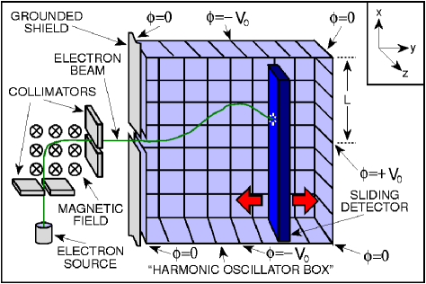
FIG. 1.: The density matrix measurement apparatus.

The Wigner phase space distribution $W$ of a 1D quantum particle is related to its density matrix $\rho$ by [25]

$$W(x,p)={1\over 2\pi}\int\rho\left(x-{u\over 2},x+{u\over 2}\right)e^{ipu}du,$$ (2)

i.e., essentially by an inverse Fourier transform in the off-diagonal direction followed by a $45^{\circ}$ rotation. Since the Hamiltonian for an electron inside our box is quadratic in positions and momenta, it is well-known [25, 26, 27] that the time-evolution of the phase space distribution $W$ is purely classical, given by the Liouville equation.

The motion is clearly independent in the $x-$, $y-$ and $z-$directions, corresponding to a harmonic oscillator, an upside down harmonic oscillator and a free particle, respectively. Since slower electrons will curve more in the magnetic field to the left of the box, it is easy to arrange for our electron beam to be highly monochromatic, with $\Delta p_{y}\ll\langle{p_{y}}\rangle$. In this limit, the marginal Wigner distribution for the $x-$direction will evolve as

$$W_{t}(x,p)=W_{0}(x\cos\theta-p\sin\theta,x\sin\theta+p\cos\theta),$$ (3)

where we have defined $\theta\equiv\omega t$ and

$$\omega\equiv\sqrt{2V_{0}|q_{e}|\over L^{2}m_{e}}.$$ (4)

We have chosen our units so that $m\omega=1$, to avoids cumbersome conversion factors between position and momentum. In other words, the time evolution simply corresponds to a clockwise rotation of the Wigner function, as shown in Figure 2.

III HOW IT WORKS

Defining $t=0$ as the time when a particle passes $y=0$ (the origin of coordinates is at the center of the box) and $p_{y0}$ as $\langle{p_{y}}\rangle$ at that time, we can make the identification

$$y=p_{y0}\sinh\theta,$$ (5)

since $\Delta p_{y}\ll\langle{p_{y}}\rangle$ at all times (particles with small $y$-momentum have been rejected by the collimators). When the slidable detector is positioned at $y$, it will thus detect the probability density

$$\rho(x)=\int W_{t}(x,p)dp,$$ (6)

where $t=\theta/\omega$ is given by equation (5). Substituting equation (3) into equation (6), we can rewrite the integral as

$$\rho(x)=\int\int\delta(\widehat{\bf n}\cdot{\bf r}-x)W_{0}({\bf r}),$$ (7)

where ${\bf r}\equiv(x,p)$ and $\widehat{\bf n}\equiv(\cos\theta,\sin\theta)$. We recognize the right hand side of equation (7) as the very definition of the Radon transform of $W_{0}$, conventionally denoted $\breve{W}_{0}(\widehat{\bf n},x)$. The Radon transform has a simple geometrical interpretation: $\breve{W}_{0}(\widehat{\bf n},x)$ is the marginal distribution of $W_{0}$ projected onto a line parallel to the vector $\widehat{\bf n}$. The two “shadows” shown in Figure 2 are the marginal distributions for $x$ and $p$, corresponding to $\theta=0$ and $\theta=\pi/2$, respectively. In X-ray tomography, one measures the integral of the integrated X-ray opacity through say a patient’s head, as seen from a large number of angles $\theta$, and then wishes to reconstruct the 2D cross section. We can do “phase space tomography” and obtain “X-ray images” of the Wigner function from different angles by sliding the detector (changing $\theta$).

FIG. 2.: How “phase-space tomography” works. Shifting the detector to the right corresponds to rotating the Wigner function as the arrow shows, so that the detector measures the marginal distribution seen from a different angle in phase space. The marginal position and momentum distributions (shaded) correspond to $\theta=0$ and $\theta=\pi/2$, respectively.

The Radon transform is closely related to the Fourier transform, and it can we shown that [28]

$$\int e^{irx}\breve{W}_{0}(\widehat{\bf n},x)dx=\widehat{W}_{0}(\widehat{\bf n}r),$$ (8)

where $\widehat{W}_{0}$ is the 2D Fourier transform of $W_{0}$. The Fourier transform of the Wigner function is often called the characteristic function, and substituting equation (7) into equation (8), we thus find that the characteristic function is given by simply

$$\widehat{W}_{0}(\widehat{\bf n}r)=\int e^{irx}\rho(x)dx=\widehat{\rho}^{*}(r).$$ (9)

In other words, when we Fourier transform the probability distribution measured by the detector, we obtain a radial strip of the characteristic function. Sliding the detector to a new location gives another radial strip, etc. When we have covered phase space densely enough with such strips, we perform a 2D inverse Fourier transform (with respect to $x$ and $p$ this time, not with respect to the radius $r=\sqrt{x^{2}+p^{2}}$) and obtain our desired Wigner function. Alternatively, we can compute the density matrix directly from $\widehat{W}$ as

$$\rho(x,x^{\prime})={1\over 2\pi}\int\widehat{W}(k,x^{\prime}-x)e^{i(x+x^{\prime})k/2}dk.$$ (10)

Figure 2 shows the Wigner function corresponding to a pure state where the wavefunction is the sum of two Gaussians separated by 10 standard deviations, a very crude model of the state of an electron after passing through a double slit. When the detector is at the center of the box, at $y=\theta=0$, it would measure the double-humped marginal distribution for $x$ shown. Moving to the right in the box, the Wigner function rotates, the two humps start overlapping, and interference fringes begin to appear on the detector, finally giving the marginal distribution for $p$ (also shown in Figure 2) when $\theta=\pi/2$. Destroying the coherence of the electrons (the purity of the quantum state) would correspond to removing the oscillatory center of the Wigner function in the figure[8]. Thus no fringes would appear as we moved the detector, and the two Gaussians would merely add incoherently when they overlapped at $\theta=\pi/2$.

IV REAL WORLD ISSUES

A How to chose the voltage

Let us rewrite equation (5) as

$$y=\left({\sinh\theta\over\sinh\theta_{max}}\right)L,$$ (11)

where $\theta_{max}\equiv\sinh^{-1}[(2V_{0}|q_{e}|m_{e})^{1/2}/p_{y0}]$. To be able to “X-ray” the Wigner function from all angles $-\pi/2\leq\theta\leq\pi/2$, we clearly want $\theta_{max}\geq\pi/2$. On the other hand, it is not feasible to make $\theta_{max}$ much larger than this, since the required voltage $V_{0}$ eventually grows exponentially with $\theta_{max}$. We therefore suggest chosing $\theta_{max}$ only slightly larger than $\pi/2$, to allow for the finite thickness off the detector and room for optional double slits etc. on the left hand side. This produces classical trajectories such as

$$x{\mathrel{\hbox to0.0pt{\lower 3.0pt\hbox{$\mathchar 536\relax$}\hss}\raise 2.0pt\hbox{$\propto$}}}\cos\>\sinh^{-1}\left[2.3{y\over L}\right],$$ (12)

the beam curve in Figure 1, and means that $V_{0}$ will be about five times the potential that initially accelerated the incident electrons.

B Overcoming the resolution

If the detector registers $N$ hits, we must smooth the measured $\rho$ on the scale of their mean separation $2L/N$ to suppress Poisson shot noise. We thus define the spatial resolution $\Delta x$ as either $2L/N$ or the intrinsic resolution of the detector, whichever is larger. The $\widehat{W}$ that we measure will thus be near the true $\widehat{W}$ within a circle of radius $\sim 1/\Delta x$ but tend to zero at larger radii. This means that its Fourier transform, the Wigner function, will have a resolution of order $\Delta x$. (Recall that the $x-p$ conversion factor is $m_{e}\omega$, so the momentum resolution $\Delta p=m_{e}\omega\Delta x.$) Features on smaller scales will be washed out, and it is well-known that smearing the Wigner function tends to decrease the purity of a state, much in the same way as decoherence does. In other words, to be able to measure quantum effects with our device, not merely classical-looking mixed states, it is crucial that interference fringes be present on a scale exceeding our resolution. We can arrange this in a variety of ways, corresponding to various known ways of demonstrating visible electron interference patterns, and placing the corresponding contraptions to the left of the harmonic oscillator box. We might for instance place a crystal near the entrance of the box, whose electron diffraction pattern could be readily detectable. Alternatively, we could replace it by a microfabricated double slit magnified by electrostatic cylinder lenses, as is done in the famous electron version of Young’s double-slit experiment [29]. Also, the single opening in the box can of course be replaced by many well-separated openings, as long as they are small enough to leave the interior field approximately of the form given in equation (1).

C Other constraints

The main additional constraint is that we must ensure that the Schrödinger time evolution of equation (3) is indeed valid inside the box. Firstly, this clearly requires that the electrons evolve as an isolated system, for instance that the vacuum in the box be hard enough that the effect of air molecules can be neglected. Secondly, the electrons must only “feel” the potential of equation (1), i.e., stay inside the box. A problem of this type would of course immediately be noticed, as counts near the edge of the detector.

What number $n$ of different detector locations should we use? We saw that $\widehat{W}$ is accurately measured out to a radius $1/\Delta x$. Since each radial strip is a Fourier transform $\widehat{\rho}$, the radial resolution will be limited by the inverse length of the detector, $1/2L$. Since the resolution in the angular direction at the radius $1/\Delta x$ is just $2\pi/n\Delta x$, and for economy we want the two resolutions to be roughly equal, we should choose $n$ and $\Delta x$ such that $n\sim L/\Delta x$, i.e., so that the number of $y$-values at which we measure roughly equals the number of resolution elements on the detector.

V DISCUSSION

We have presented a method for measuring the 1D spatial density matrix (equivalently, the Wigner function) of a beam of identically prepared charged particles. Specifically, we measure the Wigner function that describes the ensemble of particles when they are at $y=0$, half way through the box. Some clarifications are in order here:

• The Wigner function at another $y$-coordinate is obtained by simply rotating the measured Wigner function by the appropriate amount.

• The reader may feel uneasy about the fact that our measurement technique assumes the validity of the Schrödinger equation. However, this per se is not that different from say measuring the velocity of a classical object, which requires position measurements at two different times and the assumption that Newton’s law of motion is valid during the interval.

• By the very definition of the density matrix, we can never measure it for a single particle, merely for an ensemble.

• The condition “identically prepared” is in a sense fulfilled by definition: if the particles in the ensemble are in fact not all in the same state, but we are unaware of this, this lack of knowledge will merely be reflected in the density matrix we measure.

The implementation of phase-space tomography presented here can obviously be generalized in a number of ways. For instance, it may be feasible to measure $\rho$ for neutral particles (discussed by [20, 21]) by replacing the box by a Stern-Gerlach type apparatus coupling to the spin, or by an electric field whose gradient couples to the dipole moment of the particles, in such a way as to produce harmonic motion in the $x$-direction. Indeed, it is easy to show that our Radon transform approach can be applied even without any external force field, for free particle time evolution. In this case, however, we never obtain quite all radial strips of $\widehat{W}$, since the Wigner function will not rotate but shear, and $\theta=\pm\pi/2$ will correspond to $t=\pm\infty$. More general stationary and time-varying potentials can of course also be used — the advantage of our quadratic potential was merely that the resulting inversion problem was linear and easy to solve.

As to the types of beams for which $\rho$ can be measured, the variations are of course many as well, employing various combinations of the above-mentioned diffracting crystals, double slits, electrostatic and magnetic lenses, etc., and adding various sources of decoherence.

In summary, it is hoped that this rather versatile technique can help us continue the trend mentioned in the introduction, and make our understanding of decoherence, quantum measurement and apparent wavefunction collapse less qualitative and more quantitative.

N.B. The latest version of this paper and related work is available from
h t t p://www.sns.ias.edu/$\tilde{~{}}$max/radon.html
(faster from the US) and from
h t t p://www.mpa-garching.mpg.de/$\tilde{~{}}$max/radon.html
(faster from Europe). Note that figure 1 will print in color if your printer supports it.

REFERENCES

- [1] P. R. Tapster, J. G. Rarity & P. C. M. Owens, Phys. Rev. Lett., 73, 1923 (1994).
- [2] P. G. Kwiat, A. M. Steinberg & R. Y. Chiao, Phys. Rev. A, 45, 7729 (1992).
- [3] E. Joos and H. D. Zeh, Z. Phys. B, 59, 223 (1985).
- [4] M. Tegmark, Found. Phys. Lett., 6, 571, (1993).
- [5] H. D. Zeh, Found. Phys., 1, 69, (1970).
- [6] W. H. Zurek, Phys. Rev. D, 24, 1516, (1981).
- [7] W. H. Zurek, Phys. Rev. D, 26, 1862, (1982).
- [8] W. H. Zurek, Phys. Today, 44 (10), 36, (1991).
- [9] J. v. Neumann, Matematische Grundlagen der Quantenmechanik (Springer, 1932).
- [10] U. Fano, Rev. Mod. Phys., 20, 74, (1957).
- [11] W. Galc, E. Guth & G. T. Trammell, Phys. Rev., 165, 1334, (1968).
- [12] J. L. Park & W. Band, Found. Phys., 1, 211, (1971).
- [13] A. Royer, Phys. Rev. Lett., 55, 2745, (1985).
- [14] A. Royer, Found. Phys., 19, 3, (1989).
- [15] J. Bertrand & P. Bertrand, Found. Phys., 17, 397 (1987).
- [16] K. Vogel & H. Risken, Phys. Rev. A, 40, 2847 (1989).
- [17] U. Leonhardt, Phys. Rev. Lett., 74, 4101 (1995).
- [18] O. Steurnagel & J. A. Vaccaro, Phys. Rev. Lett., 75, 3201 (1995).
- [19] D. T. Smithey, M. Beck, M. G. Raymer & A. Faridiani, Phys. Rev. Lett., 79, 1244 (1993).
- [20] M. G. Raymer, M. Beck & D. F. McAlister, Phys. Rev. Lett.. 72, 1137 (1994).
- [21] U. Janicke & M. Wilkens, J. Mod. Opt., 42, 2183 (1995).
- [22] M. Freyberger & A. M. Herkommer, Phys. Rev. Lett., 72, 1952 (1994).
- [23] S. Wallentowitz & W. Vogel, Phys. Rev. Lett., 75, 3201 (1994).
- [24] T. J. Dunn. I. A. Walmsley & S. Mukamel, Phys. Rev. Lett., 74, 884 (1995).
- [25] E. P. Wigner, Phys. Rev., 40, 749, (1932).
- [26] M. Hillery et al, Phys. Rep., 106, 121, (1984).
- [27] Y. S. Kim & M. E. Noz, Phase Space Picture of Quantum Mechanics: Group Theoretical Approach (World Scientific, Singapore, 1991).
- [28] I. M. Gel’fand et al, Generalized Functions, Vol. 5 (Academic Press, New York, 1966).
- [29] C. Jönsson, Z. Phys, 161, 454, (1961).