Time-of-arrival in quantum mechanics

Abstract

We study the problem of computing the probability for the time-of-arrival of a quantum particle at a given spatial position. We consider a solution to this problem based on the spectral decomposition of the particle’s (Heisenberg) state into the eigenstates of a suitable operator, which we denote as the “time-of-arrival” operator. We discuss the general properties of this operator. We construct the operator explicitly in the simple case of a free nonrelativistic particle, and compare the probabilities it yields with the ones estimated indirectly in terms of the flux of the Schrödinger current. We derive a well defined uncertainty relation between time-of-arrival and energy; this result shows that the well known arguments against the existence of such a relation can be circumvented. Finally, we define a “time-representation” of the quantum mechanics of a free particle, in which the time-of-arrival is diagonal. Our results suggest that, contrary to what is commonly assumed, quantum mechanics exhibits a hidden equivalence between independent (time) and dependent (position) variables, analogous to the one revealed by the parametrized formalism in classical mechanics.

I Introduction

Consider the following experimental arrangement. A particle moves in one dimension, along the $x$ axis. A detector is placed in the position $x=X$. Let $T$ be the time at which the particle is detected, which we denote as the “time-of-arrival” of the particle at $X$. Can we predict $T$ from the knowledge of the initial state of the particle?

In classical mechanics, the answer is simple. Let $x(t;x_{0},p_{0})$ be the general solution of the equations of motion corresponding to initial position and momentum $x_{0}$ and $p_{0}$ at $t=0$. We obtain the time-of-arrival $T$ as follows. We invert the function $x=x(t;x_{0},p_{0})$ with respect to $t$, obtaining the function $t(x;x_{0},p_{0})$. The time of arrival $T$ at $X$ of a particle with initial data $x_{0}$ and $p_{0}$ is then

$$T=t(X;x_{0},p_{0}).$$ (1)

Two remarks are in order. First, if $t(x;x_{0},p_{0})$ is multivalued, we are only interested in its lowest value, since the particle is detected the first time it gets to $X$. Second, for certain values of $x_{0}$ and $p_{0}$, it may happen that $X$ is outside the range of the function $x(t;x_{0},p_{0})$. This indicates that the detector in $X$ will never detect a particle with that initial state. The time-of- arrival is a physical variable that –in a sense– can take two kinds of values: either a real number $T\in{\rm I}\!{\rm R}$, or the value: “$T$ = never”. Notice that in the latter case, the quantity $T$ formally computed from (1) turns out to be complex. Thus, a complex $T$ from (1) (for given $X;x_{0},p_{0}$) means that the particle with initial data $x_{0},p_{0}$ is never detected at $X$.

In quantum mechanics, the problem is surprisingly harder. In this case the time of arrival can be determined only probabilistically. Let $\pi(T)$ be the probability density that the particle is detected at time $T$. Namely, let

$$\int_{T_{1}}^{T_{2}}\pi(T)dT$$ (2)

be the probability that the particle is detected between the time $T_{1}$ and the time $T_{2}$. How can we compute $\pi(T)$ from the quantum state, e.g. from the particle’s wave function $\psi(x)$ at $t=0$?

To the best of our knowledge, this question has not received a complete treatment in the standard literature on quantum mechanics. The problem of computing the time of detection of a particle is usually treated in very indirect manners. For instance, the probability (in time) of detecting a decay product – say a particle escaping the potential of a nucleus– can be obtained from the time evolution of the probability that the particle is still within the confining potential. Alternatively, one can treat the detector that measures the time-of-arrival quantum-mechanically, and compute the probabilities for the positions of the detector pointer at a later time; in this way one can trade a meaurement of the time-of-arrival for a measurement of position at a late fixed time. In the fifties, Wigner considered the problem of relating the energy derivative of the wave function’s phase shift to the scattering delay of a particle [1]. This approach, later developed by Smith [2] and others (see for instance Gurjoy and Coon [3]) gives the average delay, but fails to provide the full probability distribution of the time of arrival. (Smith’s paper begins with: “It is surprising that the current apparatus of quantum mechanics does not include a simple representation for so eminently observable a quantity as the lifetime of metastable entities.”) In the seventies, Piron discussed the problem in a conference proceeding [4], sketching ideas related to the ones developed here. Ideas related to the ones presented here were explored in ref. [5], but in this case too only the average time-of-arrival was obtained, and not its full probability distribution. Kumar [6] studied the quantum first passage problem in a path integral approach, but did not obtain a positive probability density. The problem has been studied in the framework of Hartle’s generalized quantum mechanics [7] by using sum over histories methods. Various attempts in this direction and discussions of difficulties can be found in Ref. [8]. See also the recent paper ref. [9] for a discussion of the problem and for references; in particular, ref. [9] discusses the difficulties one has to face in trying to compute sequences of times-of-arrival – an important problem which, however, we do not address here. As stressed by Hartle in [9], generalized quantum mechanics generalizes “usual quantum mechanics”; here, on the other hand, we are interested in the question whether $\pi(T)$ can be computed within the mathematical framework of conventional Hamiltonian  quantum mechanics.

We see two reasons of interest for discussing the problem of computing time-of-arrival in quantum mechanics. First, it is a well posed problem in simple quantum theory, and there must be a solution. Echoing Smith [2], we do not expect that quantum mechanics could fail to predict a probability distribution that can be experimentally measured by simply placing a detector at a fixed position and noting the time at which it “clicks”. The problem is not just academic: it is related to the problem of computing the full probability distribution (as opposed to the expectation value) for the tunnelling time through a potential barrier. This problem has relevance, for instance, in computing rates of chemical reactions (see, for example, Kumar [6]). Second, the problem bears directly on the interpretation of quantum theories without Newtonian time [14, 15] and thus on quantum gravity; we shall briefly comment on this issue in closing.

This paper is the first of a sequence of two. Here we develop a general theory for the time-of-arrival operator, and study the free nonrelativistic particle case in detail. In a companion paper [10], we investigate a technique for the explicit construction of the time-of-arrival operator in more general cases, we extent our formalism to parametrized systems, and we study some less trivial models: a particle in an exponential potential and a cosmological model.

In the next section we give a general argument, based on the superposition principle, for the existence of an operator $\hat{T}$ (the time-of-arrival operator) such that $\pi(T)$ can be obtained from the spectral decomposition of $\psi(x)$ in eigenstates of $\hat{T}$, in the usual manner in which probability distribution are obtained in quantum theory. $\hat{T}$ has peculiar properties that distinguish it from conventional quantum observables. We give a general argument based on the correspondence principle indicating that $\hat{T}$ can be expressed in terms of position and momentum operators by the inverse of the classical equations of motion, eq. (1). This does not suffice in fixing the operator, since factor-ordering ambiguities can be serious. The problem of the actual construction of the operator $\hat{T}$ in more general systems will be addressed in [10]. In Section 3 we study an explicit form of the operator in the case of a free nonrelativistic particle. We diagonalize the operator, providing a general expression for the time-of-arrival probability density $\pi(T)$. In particular, we calculate $\pi(T)$ explicitly for a Gaussian wave packet. In section 4 we discuss some consequences of our construction. We notice that the existence of the operator implies that the quantum mechanics of a free particle can be expressed in a “time-representation” basis. We derive time–energy uncertainty relations. We conclude in section 5 with a general comment on the equivalence between time and position variables suggested by our results.

In the Appendix, we study whether the probability distribution we computed is reasonable, by comparing it with the one estimated indirectly using the Schrödinger current. We find that the two agree within second order in the deBroglie wavelength of the particle. The probability computed from the Schrödinger current cannot be physically correct to all orders because it is not positive definite; whether or not the probability distribution computed with $\hat{T}$ is physically correct to all orders is a question that can, perhaps, be decided experimentally.

II Time-of-arrival: general theory

A The incomplete spectral family $P(T)$

Consider the quantum analog of the experimental situation sketched at the beginning of the paper: a particle is in an initial state $\psi$ at $t=0$, and a particle detector is placed at $x=X$. Let $T$ be the time at which the particle is detected. Let $\pi_{\psi}(T)dT$ be the probability that the particle is detected between times $T$ and $T+dT$. Let $\psi$ and $\phi$ be two quantum states such that both $\pi_{\psi}(T)$ and $\pi_{\phi}(T)$ have support in the interval $I=(T,T+\Delta T)$. Consider the state formed as the linear combination $a\psi+b\phi$ (where $a$ and $b$ are any two complex numbers with $|a|^{2}+|b|^{2}=1$).

According to the superposition principle, if a measurable quantity has a definite value $\lambda_{\psi}$ when the system is in the state $\psi$ and value $\lambda_{\phi}$ when the system is in the state $\phi$, then a measurement of such a quantity in the state $a\psi+b\phi$ will yield either $\lambda_{\psi}$, or $\lambda_{\phi}$ (with respective probabilities $|a|^{2}$ and $|b|^{2}$) [11]. If we assume the general validity of the superposition principle, we must then expect that the probability distribution $\pi_{a\psi+b\phi}(T)$ will have support in the interval $(T,T+\Delta T)$ as well. Therefore, the states $\psi$ such that $\pi_{\psi}(T)$ has support on a given interval $I=(T,T+\Delta T)$ form a linear subspace of the state space. We can therefore define a projection operator $P_{I}$ as the projector on such a subspace.

The superposition principle could fail for the time-of-arrival. However, we would be surprised if it did. Notice that the question can (probably easily) be decided experimentally. Perhaps an experiment testing the validity of the superposition principle in this contest could have some interest. Here, we assume that the principle holds, and thus the projectors $P_{T,T+\Delta T}$ are well defined.

By their very definition, the projectors satisfy $P_{I}P_{J}=P_{J}$ if the interval $J$ is contained in the interval $I$, and $P_{I}P_{J}=0$ if the two intervals are disjoint. The operators $P_{I}$ can therefore be written in terms of a family of (spectral) projectors $P(T)$ as

$$P_{T,T+\Delta T}=\int_{T}^{T+\Delta T}P(T^{\prime})dT^{\prime}.$$ (3)

The (spectral) family $P(T)$ contains all the information needed to compute $\pi(T)$. Indeed, from the definition given, and using again the superposition principle, we have easily

$$\pi_{\psi}(T)=\left\langle\,\psi\,\right|P(T)\left|\,\psi\,\right\rangle.$$ (4)

Thus the probability distribution $\pi(T)$ can be obtained in terms of the spectral family $P(T)$, in the same way in which all probability distributions are obtained in quantum mechanics. Indeed, recall that if $\hat{A}$ is the self-adjoint quantum operator corresponding to the observable quantity $A$, then the probability distribution $\pi_{\psi}(A)$ of measuring the value $A$ on the state $\psi$ is $\left\langle\,\psi\,\right|P(A)\left|\,\psi\,\right\rangle$, where $P(A)$ is the spectral family associated to $\hat{A}$, namely

$$\hat{A}=\int A\ P(A)\ dA.$$ (5)

B The operators $\hat{T}$ and $\hat{\bf P}$

One may be immediately tempted to define a “time-of-arrival operator” in analogy with (5) as

$$\hat{T}=\int_{-\infty}^{+\infty}TP(T)dT$$ (6)

so that an eigenstate of this operator with eigenvalue $T$ would be a (generalized) state detected precisely at time $T$. However, there is an important difference from usual self-adjoint quantum mechanical observables that must be addressed before doing so. If $P(A)$ is the spectral family of a self-adjoint operator $\hat{A}$, then

$$\int_{-\infty}^{+\infty}P(A)\ dA=\hat{1},$$ (7)

where $\hat{1}$ is the identity operator. On the other hand, define $\hat{\bf P}$ by

$$\hat{\bf P}:=\int_{-\infty}^{+\infty}P(T)\ dT;$$ (8)

there is no reason for $\hat{\bf P}$ to be the identity. If it is not, we say that the spectral family $P(T)$ is “incomplete”.

Incompleteness occurs because it is not true that any state is certainly detected at some time. Most likely, there are states that are never detected, given that such states exist in the classical theory as well. Thus, $\hat{\bf P}$ projects on the subspace ${\cal H}_{\rm detected}$ formed by the states in which the particle is detected at some time at $X$, and $(\hat{1}-\hat{\bf P})$ is the projector on the subspace ${\cal H}_{\rm never\,detected}$ of states in which the particle is never detected at $X$. The fact that those two classes of states form orthogonal linear subspaces follows from the superposition principle again.

Thus, $\hat{T}$ is properly defined by (6) on ${\cal H}_{\rm detected}$ only. If we define the time-of-arrival operator by (6) on the entire state space, then we have the awkward consequence that the states in the range of $P(T=0)$ and the ones in ${\cal H}_{\rm never\,detected}$ are both annihilated by $\hat{T}$. Namely $\hat{T}$ does not distinguish the states in which the particle is detected at $T=0$ from the ones in which it is never detected.

The full information that we need in order to compute $\pi(T)$ is contained in the incomplete spectral family $P(T)$, or, equivalently, in the two mutually commuting operators $\hat{\bf P}$, and $\hat{T}$, where $\hat{T}$ is a self-adjoint operator on the Hilbert space ${\cal H}_{\rm detected}=Range(\hat{\bf P}(x))$.

Notice that

$$\langle\hat{T}\rangle_{\psi}=\frac{\left\langle\,\psi\,\right|\hat{\bf P}\hat{T}(x)\hat{\bf P}\left|\,\psi\,\right\rangle}{\left\langle\,\psi\,\right|\hat{\bf P}\left|\,\psi\,\right\rangle}$$ (9)

is the expected time-of-arrival in those states that are detected at all, and is thus a conditional expectation value.

As defined in (6), $\hat{T}$ annihilates all states in ${\cal H}_{\rm never\ detected}$. It is useful to replace this definition by fixing the following convention for the action of $\hat{T}$ on ${\cal H}_{\rm never\ detected}$. We define $\hat{T}$ on the entire  state space, by mimicking what happens in classical mechanics: we choose (arbitrarily, at this stage) a (diagonalizable) action of $\hat{T}$ on ${\cal H}_{\rm never\ detected}$ with a complex (non-real) spectrum, with the understanding that any complex eigenvalue be interpreted as “the particle is never detected”. If we use this convention, the operator $\hat{T}$ is not self-adjoint, but it still has a complete and orthogonal basis of eigenstates. The reason for such a convention (which we postulate from now on) will be given below; its utility will be particularly clear in [10].

C Partial characterization of $\hat{T}$ from its classical limit

In the previous section we have argued on general grounds that a time-of-arrival operator $\hat{T}$ giving the time-of-arrival probability distribution should exist. How can we construct the operator $\hat{T}(x)$, from the knowledge of the dynamics of the system? Let us work in the Heisenberg picture. The quantum theory is defined by the Heisenberg state space, in which states do not evolve. Let $\psi$ be a Heisenberg state. The elementary operators are Heisenberg position operator $\hat{x}_{0}$ and the momentum operator $\hat{p}_{0}$, representing position and momentum at $t=0$. Since all operators can be constructed in terms of $\hat{x}_{0}$ and $\hat{p}_{0}$, we expect to be able to express $\hat{T}$ as an operator function of $\hat{x}_{0}$ and $\hat{p}_{0}$. A key requirement on $\hat{T}$ is that it yield the correct results in the classical limit (Bohr’s correspondence principle). If so, the dependence of $\hat{T}$ on $\hat{x}_{0}$ and $\hat{p}_{0}$ should reduce to the classical dependence of $T$ on $x_{0}$ and $p_{0}$ in the classical limit. This indicates that the dependence of the operator $\hat{T}$ on $\hat{x}_{0}$ and $\hat{p}_{0}$ is given by some ordering of the function (1), which, we recall, was obtained by inverting the solutions $x(t;x_{0},p_{0})$ of the classical equations of motion. Thus, we should have that

$$\hat{T}=t(X;\hat{x}_{0},\hat{p}_{0})$$ (10)

where an ordering has to be chosen. The $c$-number $X$, we recall, is the position of the detector. Notice at this point the usefulness of the convention that complex eigenvalues represent non-detection: this can go through naturally in the classical limit. Eq. (10) does not suffice in general for characterizing $\hat{T}$ uniquely, because the correct physical ordering of the operator function can be highly non-trivial. In the companion paper [10], we investigate a technique for constructing the operator $\hat{T}(X)$ and fixing the ordering ambiguities.

In order to emphasize the dependence of the time-of-arrival operator $\hat{T}$ on the position $X$ of the detector, we will, from now on, write the operator as $\hat{T}(X)$. Analogously, we will denote the spectral family of projectors associated to $\hat{T}(X)$ as $P(T;X)$, and the probability distribution of the time-of-arrival at $X$ as $\pi(T;X)$.

The construction above can be easily generalized to a systems with $n$ degrees of freedom. A classical state of such a system is described by a point in the $2n-$dimensional phase space $\Gamma$, with coordinates $\{z^{i},i=1\cdots 2n\}$. The dynamics is generated by the Hamiltonian $H(z^{i})$. The Hamilton equations of motion are $dz^{i}(t)/dt=\{z^{i},H\}$. The general solutions to these equations can be written as

$$z^{i}(t)=z^{i}(z^{i}_{0},t),\>i=1\cdots 2n,$$ (11)

where $z^{i}_{0}$ are $2n$ independent integration constants. In particular, we may choose as integration constants $z_{0}^{i}$ the values of $z^{i}$ at $t=0$, $z^{i}(0)$. The above equations enable us to compute the state of the system at any time $t$. We are interested in the time-of-arrival of the particle at a given value of one  of the phase space coordinates, say $z^{1}$. (Since the coordinates $z^{i}$ are arbitrary, $z^{1}$ can be any combination of dynamical variables.) To compute the time-of-arrival $T(Z)$ at $z^{1}=Z$, we solve the 1st equation of the system (11)

$$z^{1}(z^{i}_{0},t)=Z$$ (12)

with respect to $t$, obtaining $t(Z;z^{i}_{0})$. The time-of-arrival $T(Z)$ is then given by

$$T(Z)=t(Z;z^{i}_{0}).$$ (13)

Now, in the quantum theory, the constants of motion $Z^{i}_{0}$ correspond to Heisenberg operators $\hat{z}_{0}^{i}$. Eq. (10) is immediately generalized by “quantizing” (13) as

$$\hat{T}(Z)=t(Z;\hat{z}_{0}^{i}).$$ (14)

where, again, the operator $\hat{T}(Z)$ is given only up to the ordering.

Before concluding this section, we add an important comment on the seemingly puzzling case $T<0$, namely when the detection time is earlier  than $t=0$. In the classical case, the particle can be detected without being disturbed, but not so in quantum mechanics; therefore one might wonder about the meaning of a detection at $T<0$ for a particle that has a certain state at time $t=0$. The difficulty is avoided by choosing the definition of “state” appropriate to the present context. Consider the classical case first. $x_{0}$ and $p_{0}$ fix a unique solution of the equations of motion. This solution could be characterized by the values of $x$ and $p$ at any other time, or any two constants of the motion. The definition of “time-of-arrival” that avoids the problem of detection-before-preparation is the following. We are interested in the arrival time of a particle which is moving according to the (unique) solution of the equations of motion characterized by the fact that at $t=0$ the particle is at $x_{0}$ and $p_{0}$ if not disturbed. Analogously, in quantum mechanics $T$ is the time-of-arrival of a particle that at an earlier time $t$ (arbitrarily in the past) was in the (Schrödinger) state $\psi(t)$ uniquely characterized by the fact that, if not disturbed, it would evolve to the state $\psi(0)$ at $t=0$. In the last section we shall describe a general way of dealing with this situation.

To summarize: In this section we have put forward two physical hypotheses:

• The probability for the time-of-arrival $\pi(T;X)$ –an experimentally measurable quantity– can be computed by

  $$\pi_{\psi}(T;X)=\left\langle\,\psi\,\right|P(T;X)\left|\,\psi\,\right\rangle,$$ (15)

  where $P(T;X)$ are the projectors on the real component of the spectrum of a diagonalizable operator $\hat{T}(X)$. The states in the span of the non-real component of the spectrum of $\hat{T}(X)$ are never detected at $X$.

• The operator $\hat{T}(X)$ is given by a suitable choice of ordering from the equation

  $$\hat{T}(X)=t(X;\hat{x}_{0},\hat{p}_{0})$$ (16)

  or, in general, Equation (14).

The first hypothesis is motivated by our confidence in the general validity of the superposition principle. The second hypothesis is motivated by our confidence in the correspondence principle. In the next section we investigate some of the implications of these hypotheses and we illustrate the construction and the use of the operator $\hat{T}(X)$ in a simple case. More interesting models, with a non trivial $\hat{\bf P}$ operator, will be presented in the companion paper [10].

III Time-of-arrival of a free particle

Consider a nonrelativistic free particle in one dimension. Dynamics is generated by the Hamiltonian $H:=p^{2}/2m$. The solutions of the classical equations of motion are

$$x(t;x_{0},p_{0})={p_{0}\over m}\ t+x_{0}$$ (17)

The inversion of these yields the time at which a particle that at $t=0$ has initial position and momentum $x_{0},p_{0}$ is detected at the position $X$ (as in equation (1))

$$T(X)=t(X;x_{0},p_{0})={m(X-x_{0})\over p_{0}}.$$ (18)

Notice that up to problems at the point $p_{0}=0$ (problems with which we shall deal extensively later) the particle is always detected. In particular, $T(X)$ is never complex. This simplifies the setting greatly, since we may disregard the complications arising from the existence of (finite) regions of phase space in which the particle is not detected.

Let us consider the usual quantum theory of a free particle. We work in the Heisenberg picture. We have Heisenberg (non-evolving) states $\psi$, and time dependent Heisenberg position and momentum operators $\hat{x}(t),\hat{p}(t)$, expressed in terms of $\hat{x}_{0}$ and $\hat{p}_{0}$. Following the ideas of the previous section, we explore the hypothesis that the quantum probability distribution $\pi(T;X)$ of the time-of-arrival at $X$ of the particle can be computed in terms of an operator $\hat{T}(X)$ defined by a suitable ordering of the (formal) operator function

$$\hat{T}(X)={m(X-\hat{x}_{0})\over\hat{p}_{0}}.$$ (19)

Notice that the Heisenberg position operator is

$$\hat{x}(t):=e^{i\hat{H}t/\hbar}\hat{x}_{0}e^{-i\hat{H}t/\hbar}={\hat{p}_{0}\over m}\ t+\hat{x}_{0};$$ (20)

to be compared with (17): Thought rarely emphasized, classical and quantum dynamics are generically related by the equation

$$\hat{x}(t)=x(t;\hat{x}_{0},\hat{p}_{0})$$ (21)

where the RHS is an operator function corresponding to an ordering of the solution $x(t;x_{0},p_{0})$ of the classical equations of motion. In general, equation (21) is of scarce use for solving the quantum dynamics, since the associated ordering problem is serious; but in simple cases such as the free particle, we see from (20) that the natural ordering suffices.

We explore here the possibility that in the case of a free particle a natural ordering suffices for the time-of-arrival operator as well. Namely, we study the choice of a symmetric ordering for the operator (19). We thus define, tentatively,

$$\hat{T}(X):={mX\over\hat{p}_{0}}-m{1\over\sqrt{\hat{p}_{0}}}\hat{x}_{0}{1\over\sqrt{\hat{p}_{0}}}.$$ (22)

In order to study this operator, let us choose a concrete representation for the Hilbert space, namely a basis. It is convenient to use the momentum basis that diagonalizes $\hat{p}_{0}$, because this basis makes the definition of ${1\over\sqrt{\hat{p}_{0}}}$ simpler. Thus, we work in the Heisenberg-picture momentum basis. The states are represented as functions $\psi(k)\in L^{2}({\rm I}\!{\rm R})$, and the elementary operators $\hat{x}_{0}$ and $\hat{p}_{0}$ are given by

$$\hat{x}_{0}\circ\psi(k)=i\frac{d}{dk}\psi(k)\qquad\mbox{and}\qquad\hat{p}_{0}\circ\psi(k)=\hbar k\ \psi(k).$$ (23)

In terms of the above operators, we have, for example, the Heisenberg position operator (20)

$$\hat{x}(t)={\hbar k\over m}\ t+i{d\over dk}.$$ (24)

In this representation, the operator $\hat{T}(X)$ given in (22) is

$$\hat{T}(X)\circ\psi(k)=\left[-i\frac{m}{\hbar}\frac{1}{\sqrt{k}}\frac{d}{dk}\frac{1}{\sqrt{k}}+\frac{m}{\hbar}\frac{X}{k}\right]\psi(k).$$ (25)

(We always take the principal value of the square root: $\sqrt{k}=i\sqrt{|k|}$ for $k<0$.)

Notice that the $1-$parameter family of operators $\hat{T}(X)$ can be generated unitarily via translations

$$\hat{T}(X)=e^{-ikX}\hat{T}(0)e^{ikX}.$$ (26)

Therefore it is sufficient to study the operator $\hat{T}(0)$, namely we do not loose generality by assuming the detector to be at the origin. We thus put $X=0$ from now on, and drop the explicit $X$ dependence

$$\hat{T}:=\hat{T}(0)=-i\frac{m}{\hbar}\frac{1}{\sqrt{k}}\frac{d}{dk}\frac{1}{\sqrt{k}}.$$ (27)

We will be interested in the operators corresponding to other positions of the detector later on.

In the momentum representation, the eigenvalue equation for $\hat{T}$

$$\hat{T}\left|\,T\,\right\rangle=T\left|\,T\,\right\rangle,$$ (28)

becomes

$$\hat{T}\circ g_{T}(k)\equiv\left[-i\frac{m}{\hbar}\frac{1}{\sqrt{k}}\frac{d}{dk}\frac{1}{\sqrt{k}}\right]g_{T}(k)=T\ g_{T}(k).$$ (29)

where we have introduced the notation

$$g_{T}(k)\equiv\langle\,k\,|\,T\,\rangle$$ (30)

for the momentum representation of the eigenstate of $\hat{T}$. The eigenvalue equation is easily solved (in each half of the real line ($k\neq 0)$) by

$$g_{T}(k)=\left(\alpha_{+}\,\theta(k)+\alpha_{-}\,\theta(-k)\right)\sqrt{\frac{\hbar}{2\pi m}}\sqrt{k}\exp\left(\frac{i\hbar Tk^{2}}{2m}\right),$$ (31)

where $\theta(k)$ is the characteristic function of the positive half of the real line, and $\alpha_{\pm}$ are constants independent of $k$. In order to fix the relation between $\alpha_{+}$ and $\alpha_{-}$, let us act on $g_{T}(k)$ by $\hat{T}$. A simple calculation shows

$$\hat{T}\circ g_{T}(k)=T\cdot g_{T}(k)-i\sqrt{\frac{m}{2\pi\hbar}}\,\frac{\delta(k)}{\sqrt{|k|}}\>(\alpha_{+}+i\alpha_{-}).$$ (32)

Thus, in order to satisfy the eigenvalue equation, it is necessary that

$$\alpha_{-}=i\alpha_{+}.$$ (33)

At this point, we encounter a difficulty. The operator we have constructed does not have a basis of orthogonal eigenstates. This pathology destroys the possibility of giving $\hat{T}$ the interpretation we want. In the next subsection we show that the eigenstates of $\hat{T}$ are not orthogonal and we discuss a way out from this difficulty.

A Difficulties with $\hat{T}$ and a regulation

A simple calculation shows that for any two eigenstates of $\hat{T}$ with eigenvalues $T$ and $T^{\prime}$

$$\langle\,T\,|\,T^{\prime}\,\rangle\equiv\int_{-\infty}^{\infty}dk\>\overline{g_{T}(k)}g_{T^{\prime}}(k)=\frac{\hbar}{2\pi m}\int_{0}^{\infty}dk^{2}\>e^{\frac{i\hbar}{2m}k^{2}(T^{\prime}-T)}=\delta(T-T^{\prime})-\frac{i}{\pi(T-T^{\prime})}.$$ (34)

The eigenstates fail to be orthogonal. One can also see that $\hat{T}$ as defined above has no self-adjoint extensions by noticing that its deficiency indices are unequal.

This difficulty stalled us for sometime, and various attempts to circumvent the problem failed. A way out was then suggested by Marolf [12]. The idea is to seek an operator that in the classical limit would not reproduce the time-of-arrival exactly, but would rather reproduce a quantity arbitrary close to the time-of-arrival. Namely, we want to approximate the time-of-arrival with a different quantity, free from pathologies. It is easy to trace the above pathology to the singular behavior of $1/k$ at $k=0$. Even classically, a state with $k=0$ is physically disturbing: either the particle is never detected or the particle may stably sit over the detector. Therefore, we seek a small modification of (18) such that no divergences occur at $p_{0}=0$. The modified time-of-arrival can perhaps be interpreted as the outcome of a measurement by an apparatus arbitrarily similar to a perfect detector, but which does not allow the particle to stand still.

Let us introduce an arbitrary small positive number $\epsilon$. Consider a 1–parameter family of real bounded continuous odd functions ${f_{\epsilon}}(k)$ which approach $1/k$ pointwise. More precisely, we require

$${f_{\epsilon}}(k) = {1\over k}\qquad{\rm for}\qquad|k|>\epsilon$$ (36)

$$\mbox{and nonzero for all}\quad k\neq 0.$$

For instance, we may choose

$${f_{\epsilon}}(k) = {1\over k}\qquad\ \ \ {\rm for}\qquad|k|>\epsilon,$$ (37)

$${f_{\epsilon}}(k) = \epsilon^{-2}k\qquad{\rm for}\qquad|k|<\epsilon.$$ (38)

Using this, we define the regulated time-of-arrival operator as

$$\hat{T}_{\epsilon}=-i\frac{m}{\hbar}\sqrt{f_{\epsilon}(k)}\frac{d}{dk}\sqrt{f_{\epsilon}(k)},$$ (39)

to be compared with the unregulated operator (25). Notice that on any state with support on $|k|>\epsilon$ the operators $\hat{T}_{\epsilon}$ and $\hat{T}$ are equal. Their action differs only on the component of a state with arbitrary low momentum. As we shall see, the probability distribution for the time-of-arrival $\pi(T)$ computed from $\hat{T}_{\epsilon}$ will turn out to be independent of $\epsilon$ for states with support away from $k=0$ –reinforcing the credibility of the regulation procedure we are using.

Let us study the operator $\hat{T}_{\epsilon}$. A key point is that $\hat{T}_{\epsilon}$ commutes with $\Theta(k)=sgn(k)=\frac{k}{|k|}$. Thus, we can choose a basis of solutions of the eigenvalue equation for $\hat{T}_{\epsilon}$ formed by functions of $k$ which have support on positive or negative $k$ only. Now $\hat{T}_{\epsilon}$ is a linear differential operator and since $f_{\epsilon}(k)\rightarrow 0$ as $k\rightarrow 0$, there is no continuity condition on its eigenstates at $k=0$. These two related properties lead to a degeneracy in the spectrum. For each eigenvalue $T$, there are two eigenstates, which we choose as having support in the $k>0,k<0$ regions respectively. Namely

$$\hat{T}_{\epsilon}\left|\,T,+\,\right\rangle_{\epsilon} = T\left|\,T,+\,\right\rangle_{\epsilon},$$ (40)

$$\hat{T}_{\epsilon}\left|\,T,-\,\right\rangle_{\epsilon} = T\left|\,T,-\,\right\rangle_{\epsilon},$$ (41)

where

$$\langle\,k\,|\,T,+\,\rangle_{\epsilon}= 0 \ \ \ {\rm for}\ k<0,$$ (42)

$$\langle\,k\,|\,T,-\,\rangle_{\epsilon}= 0 \ \ \ {\rm for}\ k>0.$$ (43)

We introduce the notation

$${{}_{\epsilon}g}^{\pm}_{T}(k)\equiv\langle\,k\,|\,T,\pm\,\rangle_{\epsilon}$$ (44)

for the momentum representation of the eigenstates of $\hat{T}_{\epsilon}$. A simple calculation shows that these are

$${{}_{\epsilon}g}^{\pm}_{T}(k)=\theta(\pm k)\sqrt{\frac{\hbar}{2\pi m}}\frac{1}{\sqrt{{f_{\epsilon}}}}\exp\left(i\frac{\hbar T}{m}\int_{\pm\epsilon}^{k}dk^{\prime}({f_{\epsilon}}(k^{\prime}))^{-1}\right).$$ (45)

Explicitly, for $|k|\geq\epsilon$ we have

$${{}_{\epsilon}g}^{\pm}_{T}(k)=\theta(\pm k)\sqrt{\frac{\hbar}{2\pi m}}\sqrt{k}\exp\left(\frac{i\hbar T}{2m}(k^{2}-\epsilon^{2})\right).$$ (46)

In order to derive various properties of these eigenstates, it is convenient to introduce new coordinates on the right and left halves of the real line, as follows.

$$Z^{\pm}(k)=\int_{\pm\epsilon}^{k}dk^{\prime}\frac{1}{{f_{\epsilon}}(k^{\prime})}.$$ (47)

In the region $|k|>\epsilon$, $Z^{\pm}(k)=(k^{2}-\epsilon^{2})/2$. In what follows, we do not need the specific form of $Z^{\pm}$ in the region $|k|<0$. Note first that in each half, the Jacobian of the coordinate transformation is non-vanishing $\forall k\neq 0$, and thus, the new coordinates are strictly monotonic. At the points $|k|=\epsilon$, $Z^{\pm}(k=\pm\epsilon)=0$ respectively. Furthermore, since $|{f_{\epsilon}}(k)|\rightarrow 0$ rapidly enough as $|k|\rightarrow 0$, we see that both $Z^{\pm}\in(-\infty,\infty)$. In terms of these coordinates, the eigenstates are

$${{}_{\epsilon}g}_{T}^{\pm}(Z^{\pm})=\sqrt{\frac{\hbar}{2\pi m}}\frac{1}{\sqrt{{f_{\epsilon}}(k(Z^{\pm}))}}e^{i\frac{\hbar}{m}T\cdot Z^{\pm}}$$ (48)

and the Hermitian inner product between two states $\psi,\phi$ is

$$\langle\,\psi\,|\,\phi\,\rangle=\sum_{\eta=+,-}\int_{-\infty}^{\infty}dZ^{\eta}{f_{\epsilon}}(k(Z^{\eta}))\overline{\psi(k(Z^{\eta}))}\phi(k(Z^{\eta})),$$ (49)

From (48,49), the orthogonality of the eigenstates is manifest:

$${}_{\epsilon}\!\langle\,T,\eta\,|\,T^{\prime},\eta^{\prime}\,\rangle_{\epsilon}=\delta_{\eta,\eta^{\prime}}\delta(T-T^{\prime}).$$ (50)

In the new coordinates, completeness too is manifest. We can get the same result in the $k$-representation with a little work:

$$\sum_{\eta=+,-}\int_{-\infty}^{\infty}dT\langle\,k\,|\,T,\eta\,\rangle_{\epsilon}\>{}_{\epsilon}\!\langle\,T,\eta\,|\,k^{\prime}\,\rangle = \frac{\hbar}{2\pi m}\sum_{\eta}\int_{-\infty}^{\infty}dT\frac{1}{\sqrt{{f_{\epsilon}}(k)}}\frac{1}{\overline{\sqrt{{f_{\epsilon}}(k^{\prime})}}}e^{i\frac{\hbar}{m}T(Z^{\eta}(k)-Z^{\eta}(k^{\prime}))}$$ (51)

$$= \sum_{\eta}\frac{\delta(Z^{\eta}(k)-Z^{\eta}(k^{\prime}))}{\sqrt{{f_{\epsilon}}(k)}\overline{\sqrt{{f_{\epsilon}}(k^{\prime})}}}=\sum_{\eta}\frac{\delta(k-k^{\prime})\theta(\eta k)}{|\partial Z^{\eta}/\partial k|\>\sqrt{{f_{\epsilon}}(k)}\overline{\sqrt{{f_{\epsilon}}(k^{\prime})}}}$$ (52)

$$= \delta(k-k^{\prime}).$$ (53)

Since it has a complete orthogonal basis of (generalized) eigenstates with real eigenvalues, $\hat{T}_{\epsilon}$ is self-adjoint.

B Time-of-arrival probability density

Following the general theory of section 2, if the particle is in the Heisenberg state $\psi(k)$, the probability density $\pi(T)$ of the time-of-arrival is the modulus square of the projection of the state on the $T$-eigenstates of the time-of-arrival operator. Since these are doubly degenerate, we have in the present case

$$\pi(T)=|{}_{\epsilon}\langle\,T,+\,|\,\psi\,\rangle|^{2}+|{}_{\epsilon}\langle\,T,-\,|\,\psi\,\rangle|^{2}.$$ (54)

If we assume that the support of $\psi(k)$ does not contain (an arbitrary small finite region $|k|<\delta$ around) the origin, we can choose $\epsilon<\delta$ and, using the explicit form (46) of the eigenstates, we obtain the following expression for $\pi(T)$

$$\pi(T)=\frac{\hbar}{2\pi m}\left(\left|\int_{0}^{\infty}dk\sqrt{k}\exp\left(\frac{iT\hbar(k^{2}-\epsilon^{2})}{2m}\right)\psi(k)\right|^{2}+\left|\int^{0}_{-\infty}dk\sqrt{k}\exp\left(\frac{iT\hbar(k^{2}-\epsilon^{2})}{2m}\right)\psi(k)\right|^{2}\right).$$ (55)

Notice that the $\epsilon$ dependence gives only a phase that disappears when we take the absolute value squared. Namely

$$\pi(T)=\frac{\hbar}{2\pi m}\left(\left|\int_{0}^{\infty}dk\sqrt{k}\exp\left(\frac{iT\hbar k^{2}}{2m}\right)\psi(k)\right|^{2}+\left|\int^{0}_{-\infty}dk\sqrt{k}\exp\left(\frac{iT\hbar k^{2}}{2m}\right)\psi(k)\right|^{2}\right).$$ (56)

We thus have the result that for the states that do not include an amplitude for zero velocity, the time-of-arrival probability distribution computed (with $\epsilon$ sufficiently small) with the regulated operator $\hat{T}_{\epsilon}(x)$ is independent from $\epsilon$.

The two terms in (56) correspond to the left and right moving component of the state. Therefore, we have immediately that the probability $\pi^{+}(T)$ (and $\pi^{-}(T)$) that the particle is detected in $X=0$ while moving in the positive (or negative) direction is

$$\pi^{\pm}(T)=\frac{\hbar}{2\pi m}\left|\int_{0}^{\pm\infty}dk\sqrt{k}\exp\left(\frac{iT\hbar k^{2}}{2m}\right)\psi(k)\right|^{2}.$$ (57)

Finally, the result generalizes immediately to the case in which the detector is not placed in the origin, but rather in an arbitrary position $X$. The eigenstates of the operator $\hat{T}_{\epsilon}(X)$

$$\hat{T}_{\epsilon}(X)\left|\,T,\pm;X\,\right\rangle_{\epsilon}=T\left|\,T,\pm;X\,\right\rangle_{\epsilon}$$ (58)

are obtained using the unitary translation operator

$$\left|\,T,\pm;X\,\right\rangle_{\epsilon}=e^{-{i\over\hbar}\hat{p}X}\left|\,T,\pm\,\right\rangle_{\epsilon}.$$ (59)

yielding

$${{}_{\epsilon}g}^{\pm}_{T;X}(k)=\langle\,k\,|\,T,\pm;X\,\rangle_{\epsilon}=e^{-ikX}{{}_{\epsilon}g}^{\pm}_{T}(k).$$ (60)

The projectors considered in section 2 are given by

$$P(T;X)=\left|\,T,+;X\,\right\rangle{}_{\epsilon}\,{}_{\epsilon}\!\left\langle\,T,+;X\,\right|+\left|\,T,-;X\,\right\rangle{}_{\epsilon}\,{}_{\epsilon}\!\left\langle\,T,-;X\,\right|.$$ (61)

The probability density of being detected at time $T$ by a detector in $X$ that detects particles traveling with positive (negative) velocity is

$$\pi^{\pm}(T;X)=\frac{\hbar}{2\pi m}\left|\int_{0}^{\pm\infty}dk\sqrt{k}\exp\left(\frac{iT\hbar k^{2}}{2m}-ikX\right)\psi(k)\right|^{2}.$$ (62)

Equation (62) represents our final result for the probability distribution of the time-of-arrival at $X$ of a free quantum particle.

C Time-of-arrival of a Gaussian wave packet

As an example of an application of the above result, we compute the probability distribution for the time-of-arrival of a Gaussian wave packet. Consider a Gaussian wavepacket localized about a point (say) to the left of the origin at time $t=0$, and moving (say) to the right. In the standard Schrödinger-picture position representation, let this wave packet be given by the following normalized solution of the Schrödinger equation

$$\psi(x,t)=\left(\frac{\delta^{2}}{2\pi}\right)^{\frac{1}{4}}\frac{e^{-k_{0}^{2}\delta^{2}}}{\sqrt{\delta^{2}+\frac{it\hbar}{2m}}}\exp\left(\frac{(2\delta^{2}k_{0}+i(x-x_{0}))^{2}}{4\delta^{2}+2i\hbar t/m}\right).$$ (63)

Expectation values are as follows

$$\left\langle p(t)\right\rangle=\hbar k_{0} \left\langle\Delta p(t)\right\rangle=\frac{\hbar}{2\delta}$$ and (64)

$$\left\langle x(t)\right\rangle=x_{0}+\hbar k_{0}t/m \left\langle\Delta x(t)\right\rangle=\delta\sqrt{1+\frac{t^{2}\hbar^{2}}{4\delta^{4}m^{2}}}.$$ and (65)

If we choose $|x_{0}|>>\delta$, $|k_{0}|\delta>>1$, $x_{0}<0$ and $k_{0}>0$, this state represents a particle well localized to the left of the origin and with a well-defined positive momentum at time $t=0$. In the Heisenberg-picture momentum representation (23), this state is given by

$$\psi(k)=\left(\frac{2\delta^{2}}{\pi}\right)^{\frac{1}{4}}\exp\left(-(k-k_{0})^{2}\delta^{2}-ikx_{0}\right).$$ (66)

The envelope of this wave function is a Gaussian of width $1/\delta$ centered at $k_{0}$.

Using the theory developed, we can compute the projection of this state on the eigenstates of the time-of-arrival operator. We assume here that $\epsilon$ can be taken arbitrarily close to $0$. (See [13] for the relevant integrals). We obtain

$${}_{\epsilon}\langle\,T,+;X\,|\,\psi\,\rangle = \sqrt{\frac{\hbar}{m}}\left(\frac{\delta^{2}}{2^{5}\pi^{3}}\right)^{1/4}e^{-\delta^{2}k_{0}^{2}}\>\Gamma(5/4)\times$$ (68)

$$\left(\delta^{2}+\frac{i\hbar T}{2m}\right)^{-5/4}\left\{\left((2\delta^{2}k_{0}+i(X-x_{0}))\cdot\Phi\left[\frac{5}{4},\frac{3}{2},\frac{(2\delta^{2}k_{0}+i(X-x_{0}))^{2}}{4\delta^{2}+2i\hbar T/m}\right]\right.\right.$$

$$+\sqrt{\pi\left(\delta^{2}+\frac{i\hbar T}{2m}\right)} \times \left.\left.\exp\left(\frac{(2\delta^{2}k_{0}+i(X-x_{0}))^{2}}{4\delta^{2}+2i\hbar T/m}\right)\cdot{\cal L}\left[\frac{1}{4},-\frac{1}{2},-\frac{(2\delta^{2}k_{0}+i(X-x_{0}))^{2}}{4\delta^{2}+2i\hbar T/m}\right]\right)\right\},$$ (69)

$${}_{\epsilon}\langle\,T,-;X\,|\,\psi\,\rangle = \sqrt{\frac{\hbar}{m}}\left(\frac{\delta^{2}}{2^{5}\pi^{3}}\right)^{1/4}e^{-\delta^{2}k_{0}^{2}}\>\Gamma(5/4)(-i)\times$$ (72)

$$\left(\delta^{2}+\frac{i\hbar T}{2m}\right)^{-5/4}\left\{\left(-(2\delta^{2}k_{0}+i(X-x_{0}))\cdot\Phi\left[\frac{5}{4},\frac{3}{2},\frac{(2\delta^{2}k_{0}+i(X-x_{0}))^{2}}{4\delta^{2}+2i\hbar T/m}\right]\right.\right.$$

$$+\sqrt{\pi\left(\delta^{2}+\frac{i\hbar T}{2m}\right)} \times \left.\left.\exp\left(\frac{(2\delta^{2}k_{0}+i(X-x_{0}))^{2}}{4\delta^{2}+2i\hbar T/m}\right)\cdot{\cal L}\left[\frac{1}{4},-\frac{1}{2},-\frac{(2\delta^{2}k_{0}+i(X-x_{0}))^{2}}{4\delta^{2}+2i\hbar T/m}\right]\right)\right\},$$ (73)

where we have ignored the components in $|k|<\epsilon$, since $\epsilon$ can be taken arbitrarily small. ($\Phi[n,m;z]={}_{1}F_{1}[n;m;z]$ is the Kummer confluent hypergeometric function, ${\cal L}[n,a;z]={\cal L}_{n}^{a}(z)$ is the $n$th generalized Laguerre polynomial and $\Gamma(n)$ is the Euler gamma function.) The probability distribution is then given by (54). The expression above for the probability distribution of the time of arrival of a Gaussian wave packet is a bit heavy; in order to unravel its content, we have expanded it in powers of small quantities in the Appendix A, and we have plotted the total probability density $\pi(T)$ at various detector positions $X$ in Figure 1 (choosing a Gaussian state (63) with $x_{0}=-5,k_{0}=20,\delta=.5,\hbar=m=1$). To begin with, the term corresponding to negative velocities is exponentially small; indeed, it derives from the scalar product of a Gaussian wave packet concentrated around a positive $k$ with a function having support on $k<0$.

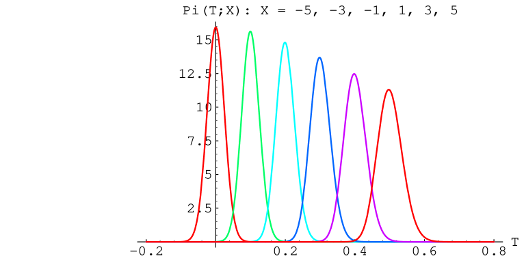
FIG. 1.: Time-of-arrival probability densities $\pi(T;X)$, plotted at the detector positions $X=-5,-3,-1,1,3,5\>$.

The total detection probability density at time $T$ for the detector in position $X$ is a function (more precisely, it is a density in $T$) on the $T-X$ plane. This function is concentrated around the classical trajectory of the particle $X=x_{0}+p_{0}T/m$, with a (quantum) spread in $T$ that increases with the spread of the wave packet, namely with the distance of the detector from the initial state.

In Appendix A, we compare our result with the probability density obtained indirectly using the Shrödinger probability density. We find good agreement within second order in the deBroglie wavelength of the particle, and we discuss the order of the discrepancies. Thus, our result is reasonable to leading order. Whether or not it is physically correct to all orders is a question that can perhaps be decided experimentally. A discrepancy with an experimental result may indicate an incorrect ordering of the time-of-arrival operator, or a more general difficulty with our approach.

IV Discussion

A Time representation

Anytime we have a self-adjoint operator in quantum mechanics, we may define a representation that diagonalises this operator. Namely, we may choose the eigenbasis of the operator as our working basis on the theory’s Hilbert space. Nothing prevents us from doing so with the operators $\hat{T}_{\epsilon}(X)$ as well. Let us therefore introduce a “time-of-arrival representation”, or, for short, a “time-representation”. We fix an $\epsilon$ and define

$$\psi^{\pm}_{\epsilon}(T,X):={}_{\epsilon}\langle\,T,\pm;X\,|\,\psi\,\rangle=\int dk\ \overline{{{}_{\epsilon}g}_{T;X}^{\pm}(k)}\ \psi(k).$$ (75)

Clearly, we can do quantum mechanics in the $\psi^{\pm}_{\epsilon}(T,X)$ representation, as well as we do quantum mechanics in the position, momentum, or energy representations. Since the eigenstates ${{}_{\epsilon}g}_{T,X}^{+}(k)$ have support on positive $k$, we must interpret $\psi^{+}_{\epsilon}(T,X)$ as the amplitude for the particle to be detected by a detector placed at $X$ in an infinitesimal neighborhood of $T$ coming from the left, and $\psi^{-}_{\epsilon}(T,X)$ as the amplitude to be detected at $X$ in a neighborhood of $T$ coming from the right.

What is the relation between the $\psi^{\pm}_{\epsilon}(T,X)$ amplitude and the conventional Schrödinger wave function $\psi(x,t)$? Notice that the first is defined by $\psi^{\pm}_{\epsilon}(T,X)={}_{\epsilon}\langle\,T,\pm;X\,|\,\psi\,\rangle$, where $\left|\,T,\pm;X\,\right\rangle{}_{\epsilon}$ is an eigenstate of $T_{\epsilon}(X)$ with eigenvalue $T$; while the second can be viewed as defined by $\psi(x,t)=\langle\,x;t\,|\,\psi\,\rangle$, where $\left|\,x;t\,\right\rangle$ is the eigenstate of the operator $\hat{x}(t)$ with eigenvalue $x$. At first sight, the two seem to be related to the same quantity (up to the $\epsilon$ and the distinction between the two directions of the velocity): they both refer to probabilities of being detected at some space-point and at some time. However, this naive observation is very misleading. The quantity $|\psi(x,t)|^{2}dx$ is the probability in space that the particle happens to be between the positions $x$ and $x+dx$ at time $t$, as opposed to being elsewhere  at time $t$. Whereas, the quantity $|\psi^{\pm}(T,X)|^{2}dT$ is the probability in time that the particle happens to arrive between times $T$ and $T+dT$ at the position $X$, as opposed to reaching $X$ at some other time . The two bases $\left|\,T,\pm;X\,\right\rangle{}_{\epsilon}$ and $\left|\,x;t\,\right\rangle$ are two well defined (generalized one-parameter families of) bases in the Hilbert space, but they are distinct.

In particular, the two bases $\left|\,T,\pm;X\,\right\rangle{}_{\epsilon}$ and $\left|\,x;t\,\right\rangle$ have distinct dimensions, because $|\psi(x,t)|^{2}\ dx$ and $|\psi^{\pm}(T,X)|^{2}\ dT$ must both be dimensionless probabilities. Thus, the transformation factor between $\left|\,T,\pm;X\,\right\rangle$ and $\left|\,x;t\,\right\rangle$ has the dimension of the square root of a velocity. Indeed, let us write the two (generalized) states explicitly in the Heisenberg momentum representation. Restricting ourselves to $k>0$ and taking $\epsilon$ to zero for simplicity, we have from (46)

$$\langle\,k\,|\,T,+;X\,\rangle{}_{\epsilon}=\sqrt{\frac{\hbar}{2\pi}}\sqrt{{k\over m}}\exp\left(\frac{i\hbar T}{2m}k^{2}-ikX\right),$$ (76)

while, as it is well known,

$$\langle\,k\,|\,x,t\,\rangle=\sqrt{\frac{\hbar}{2\pi}}\exp\left(\frac{i\hbar t}{2m}k^{2}-ikx\right).$$ (77)

Therefore, taking $x=X$ and $t=T$ we have

$$\langle\,k\,|\,T,+;X\,\rangle{}_{\epsilon}=\sqrt{{k\over m}}\ \langle\,k\,|\,x,t\,\rangle.$$ (78)

A physical understanding of the curious $\sqrt{{k\over m}}$ factor that characterizes the eigenstates of the time-of-arrival operator can be obtained as follows. Consider a well localized wave packet travelling with velocity $v=k_{0}/m$. We have approximately $|\psi^{\pm}(T,X)|^{2}\approx v\ |\psi(x,t)|^{2}$. Now, consider the $x-t$ plane. The wave function $\psi(x,t)$ is significantly different from zero on a band around the classical trajectory. The classical trajectory is a straight line with a slope given by the velocity $v$. The ratio between a vertical and an horizontal section of the band is therefore precisely $v$. Thus, in order to have both total probabilities normalized to 1 when integrating along a $t$ = constant, or a $x$ = constant line, the probability density in space and the probability density in time must be related by a factor $v$.

In Figure 2 we have plotted the usual Schrödinger probability density in $x$ – $\pi(x;t)=|\psi(x,t)|^{2}$ – at various times, for the same state used for Figure 1.

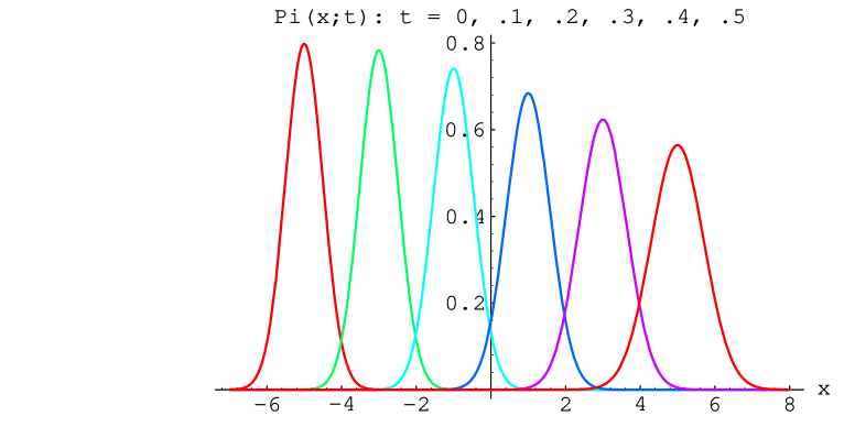
FIG. 2.: Schrödinger probability densities $\pi(x;t)$ for position, plotted at the times $t=0,.1,.2,.3,.4,.5\>$.

The time-of-arrival probability densities are $v=k_{0}/m$ times as large as the Schrödinger densities for values of $X=x$ and $T=t$ near the classical trajectory.

B Time-energy uncertainty relation

Position-momentum uncertainty relations are of wide use in quantum mechanics, and can be cleanly derived from the formalism on very general grounds. The commutation relations $[\hat{x},\hat{p}]=-i\hbar\hat{1}$ imply $\Delta x\Delta p>2h$. Time-energy uncertainty relations are of wide use as well (e.g. between the width of a spectral line and the lifetime), but their general derivation is notoriously tricky. If one tries to reproduce the position-momentum derivation for the time-energy case by assuming the existence of an operator $\hat{T}$ such that

$$[\hat{T},\hat{H}]=-i\hbar\hat{1}$$ (79)

from which

$$\Delta T\Delta E>2h$$ (80)

would follow, then one would clash against a well known non-existence theorem for $\hat{T}$. The theorem states that the commutation relations $[\hat{A},\hat{B}]=-i\hbar\hat{1}$ between two self-adjoint operators $\hat{A}$ and $\hat{B}$ implies that the spectrum of both operators is the real line. However, the spectrum of the Hamiltonian is bounded from below in all reasonable systems. Ergo  a time operator $\hat{T}$ satisfying (79) does not exist.

This theorem might have been the reason for which a time-of-arrival operator has virtually never been considered in quantum mechanics. In fact, it is often stated that time cannot be an operator in quantum mechanics, with the above theorem as a proof. Here, we show how one can rigorously derive time-energy uncertainty relations for a quantum particle, and how the existence of $\hat{T}_{\epsilon}$ circumvents the theorem.

The commutation relations between $\hat{T}_{\epsilon}$ and the Hamiltonian are easy to compute. In the momentum representation we have

$$[\hat{T}_{\epsilon},\hat{H}]=-i\hbar\hat{1}-i\hbar h_{\epsilon}(k),$$ (81)

where

$$h_{\epsilon}(k)=1-kf_{\epsilon}(k).$$ (82)

The function $h_{\epsilon}(k)$ is bounded (by $\epsilon^{2}$, if we chose $f_{\epsilon}(k)$ as in (37), which we do here for simplicity) and has support on the small interval $|k|<\epsilon$. For the particle in the state $\psi(k)$ the following uncertainty relations follow

$$\Delta T_{\epsilon}\Delta E>2h-4\pi\epsilon^{2}\int_{-\epsilon}^{+\epsilon}dk\ |\psi(k)|^{2}>2h-4\pi\epsilon^{2}.$$ (83)

By chosing $\epsilon$ sufficiently small, we obtain an uncertainty relation that approaches (80) to any desired precision.

C On the definition of state in quantum mechanics

Finally, let us return to the problem we briefly discussed at the end of section 2, which is the interpretation of the time-of-arrival $T$ when $T<0$, namely when detection time is earlier than the time $t=0$ at which the initial state is given. We have suggested that in this case the correct interpretation of $T$ is the following. $T$ is the detection time for a state that arbitrarily in the past was in a state that would have evolved to the $t=0$ initial state if undisturbed. A cleaner way of dealing with the general situation, is to make use of a fully time-independent notion of “state” and a fully time-independent version of phase space and quantum state space. This can be done as follows. Consider first classical mechanics. Let us denote a single solution of the equation of motion as a “physical history” of the system. (A physical history should not be confused with the histories considered in sum-over-histories theories: a “physical history” here is a history satisfying the equations of motion.) Let $\Gamma_{s}$ be the space of these physical histories. A point in $\Gamma_{s}$ represents an entire evolution of the system. $\Gamma_{s}$ can be coordinatized by the 2$n$ integration constants $z^{i}$. We ask for the time-of-arrival at $x$ of a system following one of the motions in $\Gamma_{s}$. This time-of-arrival is given by (13). The key to the matter is that there is no need to choose a time in order to specify a physical history.

In quantum mechanics we can define the Hilbert space ${\cal H}_{S}$ of the solutions, of the Schrödinger equation. A vector in $H_{S}$ represents an entire (quantum) motion of the system, without reference to any particular time. The conventional Heisenberg operators are defined on ${\cal H}_{S}$. The operator (14) is properly defined on ${\cal H}_{S}$. We may choose to represent the vectors in ${\cal H}_{S}$ by means of the value that the Schrödinger state would take (if undisturbed) at $t=0$; therefore it makes sense to define $\hat{T}$ as a function of the operators $x_{0}$ and $p_{0}$ which are defined on the states at $t=0$.

In this regard, it is interesting to notice that the original definition of the “Heisenberg picture Hilbert space” given by Dirac in the first edition of “Principles of Quantum Mechanics” is the definition of ${\cal H}_{S}$ given above [11]. It is only later that the “Heisenberg picture Hilbert space” came to be mostly identified with the state space at a fixed time (both interpretations of ${\cal H}_{S}$ can be found in the literature). A crucial advantage of using the definition of ${\cal H}_{S}$ given here is that this definition can be extended to systems without Newtonian time at all [14, 16]. We will exploit this point of view in [10].

V Conclusions: $x\leftrightarrow t$ equivalence in quantum theory

Let us summarize our results. We have considered the problem of computing the time-of-arrival $T$ of a quantum particle at a position $X$. Relying on the general validity of the superposition principle, we have argued that the probability distribution for $T$ can be obtained by means of an operator $\hat{T}$. This operator is, in general, not self-adjoint. However, it admits an orthogonal basis of eigenstates. The eigenstates with real eigenvalues correspond to (generalized) states for which the detection time is sharp. The eigenstates with complex eigenvalues correspond to states that are never detected.

The time-of-arrival operator is partially characterized by its classical limit, which fixes its dependence on the position and momenta operators, up to ordering. We have considered the simple case of a nonrelativistic free particle, using a tentative natural ordering. A regulation procedure allows us to to find a self-adjoint time-of-arrival operator (there is no non-detection in this case), and we have studied the probabilities the operator yields. We showed that the regulated time-of-arrival operator can be used to derive time–energy uncertainty relations, circumventing a well-known nonexistence theorem, and that it yields a well-defined “time representation” for the system.

For more general systems, the classical limit is not likely to be sufficient for constructing the operator. In a forthcoming companion paper [10] we investigate a general technique for constructing the time-of-arrival operator in general cases. We will study in detail the particle in an exponential potential, where the $\hat{\bf P}$ operator is non-trivial. We will also investigate parametrized systems and theories without a Newtonian time, arguing that the ideas presented here may be relevant for the interpretations of quantum gravity.

We close with a general comment on the significance of the result obtained. In classical mechanics there is a hidden equivalence between the independent time variable $t$ and the dependent dynamical variables –the position $x$ in the present case. This equivalence is made manifest by expressing the theory in parametrized form, namely by representing the evolution in terms of the functions $t(\tau)$ and $x(\tau)$ of an arbitrary parameter $\tau$. In more elegant and general mathematical terms, there are formulations of mechanics, e.g. the presymplectic formulation, in which the distinction between dependent and independent variables is inessential; see for instance Arnold’s classic text [17]. A parametrized representation is commonplace in special relativity (where $T$ is called $x^{0}$) since it allows manifest Lorentz covariance.

It is commonly stated that this equivalence between independent (time) and dependent variables is lost is quantum mechanics. The arguments in support of this claim are common in the quantum gravity literature and take various forms. For instance, it is said that the wave function must be normalized by integrating in $x$ and cannot be normalized by integrating in $t$. Or it is said that probabilities are always probabilities of different outcomes happening at the same time, never at the same position. It is our impression that these claims are misleading. The mistake is to assume that the $x\leftrightarrow t$ equivalence has to be realized as an equivalence in the arguments of the Schrödinger wave function $\psi(x,t)$.

The conventional formulation of quantum mechanics in terms of the Schrödinger wave function $\psi(x,t)$ has already  broken the $x\leftrightarrow t$ equivalence. Indeed, it is a formulation tailored to answer the (experimental) question: “What is the probability of the particle being here now, as opposed to that of being elsewhere now?”. The corresponding representation diagonalises the Heisenberg operators $\hat{x}(t)$. It is the experimental question considered, and the related choice of basis, that breaks the $x\leftrightarrow t$ equivalence. Quantum mechanics allows us to consider the following question as well: “What is the probability of the particle getting here now as opposed to getting here elsewhen?”. In order to answer this question, one is led naturally to the $\psi^{\pm}(T,X)$ representation in which the role of position and time are to a large extent interchanged. In particular, the wave function is normalized in time and probabilities of events at the same position are considered.

To avoid misunderstandings, let us make clear that we certainly do not claim that space and time have the same nature, nor that their role in the quantum mechanics of a particle is exactly the same. What we suggest is that the common arguments that $x$ and $t$ can be treated on equal footing in classical mechanics, but not in quantum mechanics, might loose force under closer scrutiny. Contrary to the above arguments, our analysis has revealed an underlying hidden equivalence between “dependent” and “independent” variables in the quantum theory of a free particle.

Acknowledgments

We thank Ed Gurjoy and Ted Newman for useful discussions. We are particularly grateful to Don Marolf for the suggestion of the way to regulate the time-of-arrival operator and to Jim Hartle and Jonathan Halliwel for stressing the importance of the problem and for helpful discussions and correspondence.

A Is the computed probability density reasonable ?

Let us now investigate whether the result we have obtained for the Newtonian free particle is physically reasonable. The simplest check is to compute the expectation value of the time-of-arrival of a wave packet with initial position $x_{0}$ and momentum $p_{0}$. The result should agree with the expected classical time-of-arrival $T=t(X;x_{0},p_{0})$. Since the operator was constructed via a factor-ordering and regulation of the classical solution, the expectation values obviously satisfy Ehrenfest’s theorem. A more accurate check which goes beyond the semiclassical approximation is to compare the probability distribution we have obtained with the one we can estimate by indirect but intuitive methods. In appendix A.1, we first compute an approximation to the probability amplitude (68) –and the resulting probability density– for a Gaussian state. This also gives us some intuition for the behavior of the the distribution. Then in appendix A.2, we compute the Schrödinger current through the detector position, and compare this with the approximation we will obtain in section A.1.

1 Gaussian state

Consider the Gaussian wavepacket of section 3.5. In the momentum representation, this state is given by

$$\psi(k)=\left(\frac{2\delta^{2}}{\pi}\right)^{\frac{1}{4}}\exp\left(-(k-k_{0})^{2}\delta^{2}-ikx_{0}\right).$$ (A.1)

The envelope of this wave function is a Gaussian of width $1/\delta$ at positive momentum $k_{0}$. In order to simplify the calculations, we slightly modify this state by assuming it to be zero for $k<\epsilon$. Clearly, since this modification is far out on the tail of the Gaussian, the error we make is very small (More precisely, one can show that it vanishes as $\exp{(-1/k_{0}\delta)}$). We thus replace (A.1) by

$$\psi(k)=\theta(k-\epsilon)\left(\frac{2\delta^{2}}{\pi}\right)^{\frac{1}{4}}\exp\left(-(k-k_{0})^{2}\delta^{2}-ikx_{0}\right).$$ (A.2)

where $\theta(x)$ is the characteristic function of the positive line. Substituting this expression into (75), we find that the amplitude for the particle to be detected between $T$ and $T+dT$ at the position $x$ is

$$\psi^{+}(T,X) = \sqrt{\frac{\hbar}{2\pi m}}\left(\frac{2\delta^{2}}{\pi}\right)^{1/4}\int_{\epsilon}^{\infty}dk\,\sqrt{k}\exp\left(-(k-k_{0})^{2}\delta^{2}-i\frac{\hbar T}{2m}k^{2}+ik(X-x_{0})\right)$$ (A.3)

$$= \sqrt{\frac{\hbar}{2\pi m}}\left(\frac{2\delta^{2}}{\pi}\right)^{1/4}\left[\int_{-\infty}^{\infty}dk\,\sqrt{k}\exp\left(-(k-k_{0})^{2}\delta^{2}-i\frac{\hbar T}{2m}k^{2}+ik(X-x_{0})\right)-R_{1}\right]$$ (A.4)

where $R_{1}$ is again exponentially small, $\sim\exp(-1/k_{0}\delta)$, and we have disregarded an $\epsilon$-dependent phase, which is not going to affect the probability distribution.

Now we can expand $\sqrt{k}$ about the peak of the Gaussian as

$$\sqrt{k}=\sqrt{k_{0}}\left(1+\frac{k-k_{0}}{2k_{0}}+O\left(\frac{k-k_{0}}{k_{0}}\right)^{2}\right).$$ (A.6)

Using this expansion, we can compute the Gaussian integral in (A.3)

$$\int_{-\infty}^{\infty}dk\sqrt{k}\exp\left(-(k-k_{0})^{2}\delta^{2}-i\frac{\hbar T}{2m}k^{2}+ik(X-x_{0})\right)$$ (A.7)

$$=e^{ik_{0}(X-x_{0})-i\frac{\hbar T}{2m}k_{0}^{2}}\left[\sqrt{\frac{k_{0}^{2}\pi}{\delta^{2}+i\frac{\hbar T}{2m}}}\exp\left[-\frac{(X-x_{0}-\frac{\hbar Tk_{0}}{m})^{2}}{4(\delta^{2}+i\frac{\hbar T}{2m})}\right]\left(1+i\frac{X-x_{0}-\frac{\hbar Tk_{0}}{m}}{4k_{0}(\delta^{2}+i\frac{\hbar T}{2m})}\right)+R_{2}\right],$$ (A.8)

where

$$|R_{2}|\leq\frac{1}{8k_{0}^{3/2}}\int_{-\infty}^{\infty}dk\,k^{2}e^{-k^{2}\delta^{2}}=\sqrt{k_{0}\pi}\frac{1}{16k_{0}^{2}\delta^{2}}\frac{1}{\delta}$$ (A.10)

is of second order in $1\over\delta k_{0}$. Thus, to first order in the (small) quantity $1\over\delta k_{0}$, we have

$$\psi^{+}(T;x)=\sqrt{\frac{\hbar k_{0}}{m}}\left(\frac{\delta^{2}}{\pi}\right)^{1/4}e^{ik_{0}(X-x_{0})-i\frac{\hbar T}{2m}k_{0}^{2}}\frac{\exp\left(-\frac{(X-x_{0}-\frac{\hbar Tk_{0}}{m})^{2}}{4(\delta^{2}+i\frac{\hbar T}{2m})}\right)}{4(\delta^{2}+i\frac{\hbar T}{2m})^{1/2}}\left(1+i\frac{X-x_{0}-\frac{\hbar Tk_{0}}{m}}{4k_{0}(\delta^{2}+i\frac{\hbar T}{2m})}\right),$$ (A.11)

To this approximation, the probability density $\pi^{+}(T;x)=|\psi^{+}(T;x)|^{2}$ is then

$$\pi^{+}(T;x)=\frac{\hbar}{m\sqrt{2\pi}}\frac{(k_{0}\delta^{2}+\frac{(X-x_{0})T\hbar}{4m\delta^{2}}+\frac{k_{0}(X-x_{0}-k_{0}\hbar T/m)^{2}}{16k_{0}^{2}\delta^{2}})}{\left(\delta^{2}+\frac{T^{2}\hbar^{2}}{4m^{2}\delta^{2}}\right)^{3/2}}\exp\left(-\frac{(X-x_{0}-k_{0}T\hbar/m)^{2}}{2\left(\delta^{2}+\frac{T^{2}\hbar^{2}}{4m^{2}\delta^{2}}\right)}\right).$$ (A.12)

Due to the Gaussian factor, the probability distribution is centered on the classical time-of-arrival $T=m{X-x_{0}\over\hbar k_{0}}$, with width $\delta$, and vanishes exponentially outside such a region.

Notice also that due to the Gaussian factor the third term in the numerator of the amplitude of the Gaussian is of order $(\frac{1}{\delta k_{0}})^{2}$ in all the region where the probability density is not exponentially small, so we may rewrite the probability density as

$$\pi(T;x)=\frac{\hbar}{m\sqrt{2\pi}}\frac{(k_{0}\delta^{2}+\frac{(X-x_{0})T\hbar}{4m\delta^{2}})}{\left(\delta^{2}+\frac{T^{2}\hbar^{2}}{4m^{2}\delta^{2}}\right)^{3/2}}\exp\left(-\frac{(X-x_{0}-k_{0}T\hbar/m)^{2}}{2\left(\delta^{2}+\frac{T^{2}\hbar^{2}}{4m^{2}\delta^{2}}\right)}\right),$$ (A.13)

as an approximation correct to order $(\frac{1}{\delta k_{0}})$.

2 Current

In ordinary quantum mechanics, one can define a current whose time and space components are

$$j^{0}(x,t) = \rho(x,t)=\overline{\psi(x,t)}\psi(x,t)$$ (A.14)

$$j^{i}(x,t) = \frac{\hbar}{2mi}(\overline{\psi}\partial_{i}\psi-\psi\partial_{i}\overline{\psi})(x,t),$$ (A.15)

where $\psi(x,t)$ is the quantum state in the conventional Schrödinger-picture position representation. Since the state satisfies Schrödinger’s equation, this current is conserved

$$\partial_{0}j^{0}+\partial_{i}j^{i}=0.$$ (A.16)

Consider, for a particle in one dimension, the spacetime region (a half strip) defined by $x\leq X,t_{1}\leq t\leq t_{2}$, and integrate the divergence free current over this volume. Dropping the boundary terms at $x=-\infty$, we find that the outgoing (i.e., rightward) flux of this current through the timelike boundary at $x=X$ in the time interval $(t_{1},t_{2})$ is

$$\int_{t_{1}}^{t_{2}}dt\>j_{x} \equiv \frac{\hbar}{2mi}\int_{t_{1}}^{t_{2}}dt\>\left.(\overline{\psi}\partial_{x}\psi-\psi\partial_{x}\overline{\psi})\right|_{x=X}$$ (A.17)

$$= \int_{-\infty}^{x}dx\>\rho|_{t_{1}}-\int_{-\infty}^{x}dx\>\rho|_{t_{2}}.$$ (A.18)

The last line in the above equation is the probability that the particle is found in the LHS region ($X\leq x$) at time $t_{1}$ minus the probability that the particle is found in the LHS region at a later time $t_{2}$. It is tempting to identify the flux between the times $T$ and $T+dT$ (through the timelike surface at $x=X$) of the current density

$$j_{X}(T)dT=\frac{\hbar}{m}Im\left(\overline{\psi(x,T)}\partial_{x}\psi(x,T)\right)_{x=X}dT$$ (A.19)

as the probability density that a detector placed at $x=X$ will detect the particle. Note that the Schrödinger current density has the correct dimensions of a density in time, namely $[T]^{-1}$. The problem, of course, is that the current represents the net  flux of probability across $x=X$, and thus corresponds to the difference between the probability of crossing to the right and the probability of crossing to the left. Namely we may expect that

$$j_{X}(T)\sim\pi^{+}(T;X)-\pi^{-}(T;X).$$ (A.20)

within some approximation. In fact, the current $j_{X}(T)$ is not positive definite, and we believe that this is related to the difficulties in the approaches of [8] and [6]. Equivalently, we may try to interpret the current of a pure right moving state  as the probability density that the particle crosses $x=X$. We are reassured in doing this by the fact that in this case the current is positive definite, and its integral over all times gives one. This conclusion is based on the assumption that the particle cannot “zigzag” across the $X=x$ line, an assumption which might be valid only if we look at sufficiently large times.

So, when $\psi$ is a pure right moving state, the rightward flux density is positive and integrates to 1 over all time. (To see this, take the limits $t_{1}\rightarrow-\infty$ and $t_{2}\rightarrow\infty$ in (A.17).) It is therefore at least consistent to interpret this as an estimate of the probability density. Does this estimate yield the correct semi-classical limit? The expectation values of the usual position and momentum operators satisfy Ehrenfest’s theorem, since the probability densities are associated with the decomposition of a state onto the spectrum of some self-adjoint operator. The same is true of the probability densities we have obtained from the time-of-arrival operator. The above current density is not obtained via a spectral projection, however, and is not associated with a “time operator”. How do the expectation values of the time-of-arrival behave wrt. this estimated probability density, and do they correspond to the classical limit in some way? We next proceed to analyze this issue.

The expectation value of the time-of-arrival of the particle at the position $X$ is naturally defined only when the state has support only on the $k\geq 0$ region and is then given by

$$\left\langle T\right\rangle_{X} = \int_{-\infty}^{\infty}dT\>T\,j_{X}(T)$$ (A.21)

$$= \frac{\hbar}{2\pi m}Re\left\{\int_{-\infty}^{\infty}dT\int_{0}^{\infty}dk\int_{0}^{\infty}dk^{\prime}\>T\cdot\exp\left(\frac{i\hbar Tk^{2}}{2m}-ikX\right)\overline{\psi(k)}\exp\left(\frac{-i\hbar Tk^{\prime 2}}{2m}+ik^{\prime}X\right)\psi(k^{\prime})\right\}$$ (A.22)

$$= \frac{\hbar}{2\pi m}Re\left\{\int_{-\infty}^{\infty}dT\int_{0}^{\infty}dk\int_{0}^{\infty}dk^{\prime}\>\frac{m}{\hbar}\frac{1}{k}\left[\left(\frac{1}{i}\frac{\partial}{\partial k}+X\right)\cdot\exp\left(\frac{i\hbar Tk^{2}}{2m}-ikX\right)\right]\right.\times$$ (A.24)

$$\left.\hphantom{aaaaaaa}\overline{\psi(k)}\exp\left(\frac{-i\hbar Tk^{\prime 2}}{2m}+ik^{\prime}X\right)\psi(k^{\prime})\right\}$$

$$= \frac{m}{\hbar}Re\left\{\int^{\infty}_{0}dk\>\overline{\psi(k)}\left(\frac{X}{k}-\frac{i}{k}\frac{\partial}{\partial k}\right)\psi(k)\right\}$$ (A.25)

$$\equiv mX\left\langle\frac{1}{\hat{p}_{0}}\right\rangle-\frac{m}{2}\left\langle\frac{1}{\hat{p}_{0}}\hat{x}_{0}+\hat{x}_{0}\frac{1}{\hat{p}_{0}}\right\rangle,$$ (A.26)

where we have dropped a surface term at $k=0$ since we assume that $\psi(k)_{k\rightarrow 0}\rightarrow k^{2+}$. The final expression in the above equation is the symmetric factor ordering of the classical expression $T=m(X-x_{0})/p_{0}$, thus we do recover the correct semiclassical limit.

For the localized right moving wave packet previously considered, the current is easily computed, giving

$$j_{X}(T)=\frac{\hbar}{2\pi m}Re\left[\int^{\infty}_{0}dk\exp\left(\frac{iT\hbar k^{2}}{2m}-ikX\right)\overline{\psi(k)}\cdot\int^{\infty}_{0}dk^{\prime}k^{\prime}\,\exp\left(\frac{-iT\hbar k^{\prime 2}}{2m}+ikX\right)\psi(k^{\prime})\right].$$ (A.27)

The integral can be explicitly done, yielding

$$j_{X}(T)=\frac{\hbar}{m\sqrt{2\pi}}\frac{(k_{0}\delta^{2}+\frac{(X-x_{0})T\hbar}{4m\delta^{2}})}{\left(\delta^{2}+\frac{T^{2}\hbar^{2}}{4m^{2}\delta^{2}}\right)^{3/2}}\exp\left(-\frac{(X-x_{0}-k_{0}T\hbar/m)^{2}}{2\left(\delta^{2}+\frac{T^{2}\hbar^{2}}{4m^{2}\delta^{2}}\right)}\right).$$ (A.28)

which is precisely the approximate form for the probability we computed from the time-of-arrival operator (see (A.13)). Thus, the probability distributions computed with the time-of-arrival operator and by means of the current agree for a right moving localized wave packet to order $(1/k_{0}\delta)$, which is one order beyond the classical limit.

For a general state, roughly localized in momentum state around a momentum $k_{0}$, we can compare the current (A.19) with the difference between the probability of being detected moving towards the right minus the probability of being detected moving left. Namely we can estimate

$$d_{X}(T)=j_{X}(T)-(\pi_{X}^{+}(T)-\pi_{X}^{-}(T)).$$ (A.29)

Explicitly, using (A.19) and (56), we have

$$d_{X}(T) = \frac{\hbar}{m}Im\left(\overline{\psi(X;T)}\partial_{X}\psi(X;T)\right)_{x=X}-\frac{\hbar}{2\pi m}\left|\int_{0}^{+\infty}dk\sqrt{k}\exp\left(\frac{-iT\hbar k^{2}}{2m}+ikX\right)\psi(k)\right|^{2}$$ (A.31)

$$+\frac{\hbar}{2\pi m}\left|\int_{-\infty}^{0}dk\sqrt{k}\exp\left(\frac{-iT\hbar k^{2}}{2m}+ikX\right)\psi(k)\right|^{2}.$$

We now put $X=0$ for simplicity, without loss of generality. A little algebra gives

$$d_{0}(T)=\frac{\hbar}{2\pi m}\int_{-\infty}^{+\infty}dk\int_{-\infty}^{+\infty}dk^{\prime}(\sqrt{k}-\sqrt{k^{\prime}})^{2}\exp\left(\frac{-iT\hbar(k^{2}-k^{\prime}{}^{2})}{2m}\right)\psi(k)\overline{\psi(k^{\prime})}.$$ (A.32)

Now suppose that our measurement has a precision $\delta T$. Then the difference of the probability densities, averaged around $T$ is

$$\Delta P(T,\delta T)=\frac{1}{2\delta T}\int_{T-\delta T}^{T+\delta T}dT^{\prime}\>d_{0}(T^{\prime}).$$ (A.33)

The integral in $dT^{\prime}$ can be done easily, which yields

$$\Delta P(T,\delta T)=\frac{\hbar}{2\pi m}\int_{-\infty}^{+\infty}dk\int_{-\infty}^{+\infty}dk^{\prime}(\sqrt{k}-\sqrt{k^{\prime}})^{2}e^{\left(\frac{-iT\hbar(k^{2}-k^{\prime}{}^{2})}{2m}\right)}\psi(k)\overline{\psi(k^{\prime})}\left\{\frac{\sin(\frac{\delta T\hbar}{2m}(k^{2}-k^{\prime}{}^{2}))}{\frac{\delta T\hbar}{2m}(k^{2}-k^{\prime}{}^{2})}\right\}.$$ (A.34)

For large $\delta T$, compared to the “deBroglie time” of the particle $\frac{2m}{k^{2}\hbar}$ (where $k$ is the highest momentum in the support of the wave function), the factor $\{\,\}$ in the integrand approaches a delta function in the difference between the two integration variables (plus a term with a delta function in the sum of the two integration variables, which we may assume to be negligible for states sufficiently localized in momentum space), and the integral is then suppressed by the $(\sqrt{k}-\sqrt{k^{\prime}})^{2}$ factor. This indicates that the two ways of computing the probability for the time-of-arrival approach each other when our resolution time is larger than the particle’s deBroglie time.

REFERENCES

- [1] EP Wigner, Phys Rev 98 (1955) 145.
- [2] FT Smith, Phys. Rev. 118 (1960) 349.
- [3] E Gurjoy, D Coon, Superlattices and Microstructures, 5 (1989) 305, and references therein.
- [4] C Piron, in Interpretation and foundations of Quantum Theory, ed H Newmann, Bibliographisches Institute, Manheim 1979.
- [5] VS Olkhovsky, E Recami, AJ Gerasimchuk, Nuovo Cimento 22, 262 (1974).
- [6] N Kumar, Pramana – J. of Phys. 25 4 (1985) 363-367.
- [7] JB Hartle, in Gravitation and quantification, Les Houches Ecole d’ete, 1992. Santa Barbara preprint UCSBTH92-21.
- [8] JB Hartle, Phys.Rev. D43, 1434, 1988; D44, 3173 (1991). N Yamada and S Takagi, Prog.Theor.Phys. 85, 985 (1991); 86, 599 (1991); 87, 77 (1992). J.J.Halliwell and M.E.Ortiz, Phys.Rev. D48, 748 (1993). N Yamada, Sci. Rep. Tôhoku Uni., Series 8, 12, 177 (1992). JJ Halliwell, Phys.Lett. A207, 237 (1995)
- [9] JB Hartle, ”Time and Time Functions in Parametrized Non-Relativistic Quantum Mechanics”, Santa Barbara preprint UCSBTH95-2, gr-qc/9509037.
- [10] C Rovelli and RS Tate, in preparation.
- [11] PAM Dirac, Principles of Quantum Mechanics, (Oxford University Press: Oxford 1930).
- [12] D Marolf, private communication, Pittsburgh, 1995.
- [13] IS Gradshtein and IM Ryhzik Table of integrals, Series and Products, ed. A Jeffrey (Academic Press: New York 1980) p.1064.
- [14] C Rovelli, Physical Review D43, 442 (1991); Physical Review D42, 2638 (1991).
- [15] C Isham, in Integrable systems, Quantum Groups, and Quantum Field Theories, eds LA Ibort and MA Rodriguez (Kluwer Academic Publishers: London 1993).
- [16] A Ashtekar A and RS Tate, Jour. Math. Phys. 35, 6434, 1994 and references therein; RS Tate 1992 “An algebraic approach to the quantization of constrained systems: finite dimensional examples”, Ph.D. dissertation, Syracuse University, gr-qc/9304043.
- [17] VI Arnold, Mathematical Methods of Classical Mechanics (Springer-Verlag: Berlin 1978).