LBL-35972

Quantum Electrodynamics at Large Distances II: Nature of the Dominant Singularities.

Takahiro Kawai

Research Institute for Mathematical Sciences
Kyoto University
Kyoto 606-01 JAPAN

Henry P. Stapp

Lawrence Berkeley Laboratory
University of California
Berkeley, California 94720

Accurate calculations of macroscopic and mesoscopic properties in quantum electrodynamics require careful treatment of infrared divergences: standard treatments introduce spurious large-distances effects. A method for computing these properties was developed in a companion paper. That method depends upon a result obtained here about the nature of the singularities that produce the dominant large-distance behaviour. If all particles in a quantum field theory have non-zero mass then the Landau-Nakanishi diagrams give strong conditions on the singularities of the scattering functions. These conditions are severely weakened in quantum electrodynamics by effects of points where photon momenta vanish. A new kind of Landau-Nakanishi diagram is developed here. It is geared specifically to the pole-decomposition functions that dominate the macroscopic behaviour in quantum electrodynamics, and leads to strong results for these functions at points where photon momenta vanish.

Disclaimer

This document was prepared as an account for work sponsored by the United States Government. Neither the United States Government nor any agency thereof, nor The Regents of the University of California, nor any of their employees, makes any warranty, express or implied, or assumes any legal liability or responsibility for the accuracy, completeness, or usefulness of any information, apparatus, product, or process disclosed, or represents that its use would not infringe privately owned rights. Reference herein to any specific commercial products process, or service by its trade name, trademark, manufacturer, or otherwise, does not necessarily constitute or imply its endorsement, recommendation, or favoring by the United States Government or any agency thereof, or The Regents of the University of California. The views and opinions of authors expressed herein do not necessarily state or reflect those of the United States Government or any agency thereof of The Regents of the University of California and shall not be used for advertising or product endorsement purposes.

Lawrence Berkeley Laboratory is an equal opportunity employer.

1. Introduction

A method of calculating the macroscopic and mesoscopic properties of scattering functions in quantum electrodynamics was developed in reference 1, in the context of a particular example. The large-distance behaviour was shown to be concordant with the idea that electrons propagate over large distance like stable particles in classical physics. This result is expected, and indeed is required in the interpretation of scattering experiments. But unless one is able to deduce this dominant behaviour from the theory, and exhibit a controlled non-dominant remainder, the theory would be unsatisfactory, for it would lack the power to make valid predictions in the mesoscopic regime lying between the quantum and classical realms. This regime is becoming increasingly important for technology.

The extraction from quantum electrodynamics of the correspondence-principle large-distance part plus a well-controlled non-dominant remainder is a not a trivial exercise. Difficulties arise from: 1), the spurious large-distance effects introduced by the usual momentum-space treatments of infrared divergences; 2), the singular character of the photon-propagator singularity surface $k^{2}=0$ at $k=0$; 3), the occurrence of several different types of singularities on certain singularity surfaces; and 4), the need to deal effectively with the pole-decomposition functions that control the large-distance properties. These problems were all dealt with in reference 1. But one key property was left unproved. The immediate aim of this paper is to establish this property. In the course of doing so we shall develop powerful methods for dealing with singularities arising in quantum electrodynamics.

A first problem to be faced is the weakening of the Landau-Nakanishi diagrammatic conditions for the presence of a singularity. The vanishing of the gradient of $k^{2}$ at $k=0$ renders the original versions^3,4 of these conditions trivial: they yield no condition at all, for functions that describe processes with internal photons. Improved versions that cover the $k=0$ points have been devised⁵. But these also have too many solutions: in general a continuum of essentially different diagrams all lead to any given point on the Landau singularity surface. This surplus of diagrams precludes the application of the simple known rule⁶ for the nature of the singularity on that surface.

The first part of our resolution of the problem is this: Use not the original momentum-space variables, but rather a set of nested radial coordinates and the associated angles. These variables are defined by first separating the integration region into sectors specified by the different orderings of the relative sizes of the Euclidean norms $|k_{i}|$ of the soft-photon energy-momenta $k_{i}$; then, in each sector, re-ordering the vectors $k_{i}$ by size, so that $|k_{i}|\geq|k_{i+1}|$; and finally writing

$$k_{i}=r_{1}r_{2}...r_{i}\Omega_{i},$$

where, for all $i$, $|\Omega_{i}|=1$ and $0\leq r_{i}\leq 1$.

A second problem is that we need results not for the scattering functions themselves but rather to the functions obtained from them by decomposing their meromorphic parts into sums of poles times residues. The functions obtained by this pole decomposition give the dominant large-distance behaviour. We devise a new kind of “Landau” diagram for these functions.

The specific example considered in reference 1 pertains to a Feynman graph consisting of six hard photons coupled at six vertices into a single charged-particle closed loop. These six vertices are divided into three disjoint pairs, with the two vertices in each pair linked by a charged-particle line that is associated with a momentum-energy vector that is far off mass shell. This line can, for our purposes, be shrunk to a point. This produces a (triangle) graph $G$ consisting of three internal charged-particle lines, with two hard photons attached at each of the three vertices.

We now “dress” this triangle graph $G$ with soft photons: we consider the set of graphs $\{g\}$ obtained by coupling all possible numbers of soft photons into this charged-particle loop in all possible ways. If we separate the interaction term $ie\gamma_{\mu}$ into its classical and quantum parts, in the way described in ref. 1, then all the classical interactions can be shifted to the three hard vertices, leaving only quantum vertices along the three sides of the triangle. Each of these three sides $s$ of the original triangle graph $G$ is therefore now divided into segments by a set of quantum vertices. Each segment $j$ is associated with a Feynman denominator $(p_{s}+K_{j})^{2}-m^{2}+i0$, where $K_{j}$ is some (algebraic) sum of photon momenta. The total contribution from all “classical photons”, which are the photons that are coupled into $G$ only at classical vertices, can be factored off as a single unitary operator that is independent of the non-classical remainder.

We are interested here in the properties of the individual terms of the perturbation expansion of this remainder. Each such term is represented by a Feynman graph $g$. Each soft photon is coupled on one or both ends into either a vertex or a side of the original triangle graph $G$, with $C$ couplings at vertices and $Q$ couplings on the sides.

To exhibit what are expected to be (and turn out to be) the dominant contributions to the singularity of the scattering function on the triangle-diagram singularity surface $\varphi=0$ we consider the Feynman denominator associated with each segments $j$ of side $s$ to be a pole in the $z_{s}=p_{s}^{2}$ plane, and then express the function associated with each of the three sides $s$ of the triangle as a sum over pole contributions:

$$N_{s}\prod_{j=0}^{n}[(p_{s}+K_{j})^{2}-m^{2}+i0]^{-1}=N_{s}\sum_{i=0}^{n}[((p_{s}+K_{i})^{2}-m^{2}+i0)D_{si}]^{-1},$$

where $D_{si}$ is the product over $j\neq i$ of factors $((p_{s}+K_{j})^{2}-(p_{s}+K_{i})^{2})$.

There is a pole-decomposition formula like this for each of the three sides $s$ of the triangle. The direct aim of this paper is to show that for each term consisting of photon propagators, together with three factors $f_{s,i(s)}$, one from each side $s$ of $G$, with $f_{s,i(s)}$ being the $i(s)$th term in the pole-decomposition formula $(0^{\prime})$ associated with side $s$, the contours in $\Omega_{i}$-space can be shifted so as to avoid, simultaneously, all singularities in the photon propagators and residue factors. This result plays a crucial role in our arguments. It means, for the case under study, that the part of the scattering function that comes from the meromorphic parts of the propagators can be expressed as a sum of terms, in each of which the only singularities are end-point singularities at $r_{i}=0$ and $r_{i}=1$, and three Feynman denominators, one for each of the three sides $s$ of the triangle $G$. The problems are thereby focussed on the effects of the integrals over the $r_{i}$. These are the issues resolved in papers I and III.

2. Notation

The original triangle graph $G$ is shown in ^fig1).

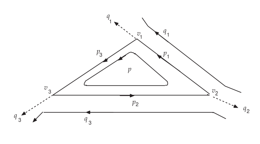
Figure 1: The basic charged–particle triangle graph $G$. The momentum–energy $p_{s}$ flows along side $s$ of the triangle in the direction of the arrow. The three energy components satisfy $p^{0}_{1}>0,$ $p_{2}^{0}<0$, and $p^{0}_{3}>0$.

The momenta $p_{1},-p_{2}$, and $p_{3}$ represent the momenta flowing from $v_{2}$ to $v_{1}$, from $v_{2}$ to $v_{3}$, and from $v_{1}$ to $v_{3}$, respectively. Conservation of energy–momentum is represented by introducing a closed loop carrying momentum $p$, and two open paths carrying momenta $q_{1}$ and $q_{3}$, respectively, in the directions indicated by the arrows. Then $p_{1}=p+q_{1},\ \ \ p_{2}=p-q_{3}$, and $p_{3}=p$.

The function associated with this Feynman graph $G$ has a singularity on the positive–$\alpha$ Landau–Nakanishi triangle–diagram singularity surface $\varphi(q)=0,$ where $q=(q_{1},q_{2},q_{3})$ and $q_{3}\equiv-q_{1}-q_{2}$. For each point $q$ on this surface $\varphi=0$ there is² a uniquely defined set of three four–vectors $p_{1}(q),p_{2}(q)$, and $p_{3}(q)$ such that the singularity at $q$ of the Feynman function $F(G)$ corresponding to the graph $G$ of Fig. 1 arises from an arbitrarily small neighborhood

$$p\approx p(q)=p_{1}(q)-q_{1}=p_{2}(q)+q_{3}=p_{3}(q)$$

in the domain of integration of the Feynman function. These three four–vectors $p_{s}(q)$ satisfy the mass–shell constraints

$$(p_{s}(q))^{2}=m^{2},$$

and the (Landau–Nakanishi) loop equation

$$\alpha_{1}p_{1}(q)+\alpha_{2}p_{2}(q)+\alpha_{3}p_{3}(q)=0,$$

where the $\alpha_{s}$ are nonnegative real numbers. This loop equation implies that for each $q$ on $\varphi(q)=0$ the three four–vectors $p_{s}(q)$ lie in some two–dimensional subspace of the four–dimensional energy–momentum space.

We shall consider a fixed interior point $q$ of the surface $\varphi=0$. In this case each of the three parameters $\alpha_{s}$ is nonzero, and each of the three four–vectors vectors $p_{s}(q)$ is nonparallel to each of the other two.

Consider now a graph $g$ obtained by inserting some finite number of soft–photon lines $i$ ($i\epsilon I$) into $G$. Each inserted line begins on a line of $G$ and ends on a line of $G$. The bound $\delta$ on the Euclidean norms $\abs{k_{i}}$ of the (soft) photon momenta is taken small enough so that

$$n\delta<\delta^{\prime}<<m,$$

where $n$ is the number of photon lines in the graph.

The case under consideration here is one where every coupling is a $Q$-type coupling. For a $C$-type coupling the corresponding vertex lies on one of the three vertices of the graph $G$. The present argument can be carried over to the case with some $C$-type couplings by simply contracting to points some segments representing residue factors, thereby bringing each of various vertices lying sides of $G$ into coincidence with a vertices of $G$. These contractions (performed after the loops have been specified) do not upset the arguments.

Momentum–energy conservation is now maintained by introducing a separate closed loop for the momentum $k_{i}$ of each photon line. Momentum $k_{i}$ flows along the photon line segment $i$ in the direction indicated by the arrow placed on that line segment. It then continues to flow through the graph $g$ by flowing along certain charged-particle lines of this graph. This continuation through $g$ is specified by the condition that this flow line pass through at most one of the three vertices $v_{1},v_{2},v_{3}$.

The arrow on photon line $i$ is chosen so that every term $p_{s}k_{i}$ that occurs in any Feynman denominator occurs with a plus sign. Consequently, the Feynman rule that $m^{2}$ represents $m^{2}-i0$ is compatible with the rule that each $p_{s}k_{i}$ represents $p_{s}k_{i}+i0$. No condition is placed on the sign of the energy component $k_{i}^{0}$.

Each charged–particle line segment $j$ has an arrow placed on it. The momentum flowing along the charged–particle segment $j$ in the direction of this arrow is called $\sum_{j}$. It is the momentum $p_{s}$ flowing along the side of the triangle upon which segment $j$ lies, as defined in Fig. 1, plus the (algebraic) sum $K_{j}$ of the photon momenta $k_{i}$ carried by the photon loops that pass along this segment $j$.

Our interest here is in the functions that arise from inserting the pole-decomposition formula $(0^{\prime})$ [or (5.5) of ref. 1] into the meromorphic parts of the generalized propagators corresponding to the three sides of the original triangle graph $G$. Consider, for example, the simple graph $g$ of ^fig2)

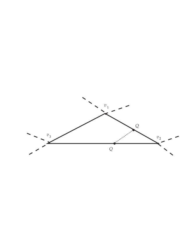
Figure 2: A graph $g$ representing a soft-photon correction to a hard-photon triangle-diagram process $G$. Hard and soft photons are represented by dashed and wiggly lines, repectively.

The meromorphic part of the function represented by the graph $g$ of Fig. 2 is a sum of the four terms represented by the four $*$ graphs of ^fig3)

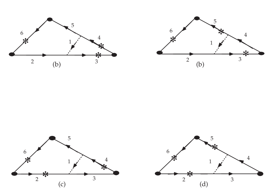
Figure 3: The $*$ graphs representing the four terms that arise from inserting the pole-decomposition formula $(0^{\prime})$ into the meromorphic part of the function represented by the graph $g$ of Fig. 2.

The asterisk $(*)$ on a line segment of a $*$ graph indicates that it is the segment associated with the (pole) denominator $(p_{s}+K_{i})^{2}-m^{2}+i0$ in the pole-decomposition formula $(0^{\prime})$. Each of the other charge–particle segments $j\neq i$ is associated with a pole–residue denominator function

$$f_{j}=2(p_{s}+K_{i})\Omega_{ij}+\rho_{ij}\Omega^{2}_{ij}+i0,$$

where

$$\rho_{ij}=r_{1}r_{2}...r_{\ell(i,j)}$$

and

$$\Omega_{ij}=(\Omega_{\ell(i,j)}+...)=\sigma_{ij}(K_{j}-K_{i})/\rho_{ij}.$$

The index $\ell(i,j)$ is the smallest $j$ such that $k_{j}$ appears in $K_{i}$ or $K_{j}$, but not both. Each of the non-exhibited terms in the parentheses in (3c) is a product of some $\pm\Omega_{k}$ with a product of a non-empty set of factors $r_{h}(h\geq 2)$.

Each of the pole-residue factors $f_{j}$ is formed by first taking the difference $\sigma_{ij}(\sum^{2}_{j}-\sum^{2}_{i})$, where $\sum_{j}=p_{s}+K_{j}$ is the momentum–energy flowing along segment $j$ in the direction of the arrow on that segment, and $\sum_{i}=p_{s}+K_{i}$ is the momentum–energy flowing along the $*$ segment on the same side $s$ of the charged–particle triangle, and then dividing out the common factors $r_{h}(h\geq 1$). The sign $\sigma_{ij}$ is the sign that makes the term $2p_{s}k_{\ell(i,j)}$ in $\sigma_{ij}(\Sigma^{2}_{j}-\Sigma^{2}_{i})$ appear with a positive sign.

The full set of functions $f_{j}$ whose zero’s define the locations of the singularities of the four functions $F_{g}$ represented by the graphs $g$ of Fig. 3 are given in Fig. 4. The functions $f_{j}$ for $j=(1,...,6)$ correspond to denominators $f_{j}+i0$. The function $f_{7}$ corresponds to the $\delta$–function constraint $\delta(\Omega\widetilde{\Omega}-1)$, and $f_{8}$ corresponds to the Heaviside function $\theta(r)$.

$$\begin{array}[]{ll}(a)&(b)\cr f_{1}=\Omega^{2}&f_{1}=\Omega^{2}\cr f_{2}=2p_{2}\Omega+r\Omega^{2}&f_{2}=2p_{2}\Omega+r\Omega^{2}\cr f_{3}=(p_{2}+r\Omega)^{2}-m^{2}&f_{3}=(p_{2}+r\Omega)^{2}-m^{2}\cr f_{4}=(p_{1}+r\Omega)^{2}-m^{2}&f_{4}=2p_{1}\Omega+r\Omega^{2}\cr f_{5}=2p_{1}\Omega+r\Omega^{2}&f_{5}=p_{1}^{2}-m^{2}\cr f_{6}=p^{2}_{3}-m^{2}&f_{6}=p^{2}_{3}-m_{2}\cr f_{7}=\Omega{\widetilde{\Omega}}-1&f_{7}=\Omega\widetilde{\Omega}-1\cr f_{8}=r&f_{8}=r\cr&\cr(c)&(d)\cr f_{1}=\Omega^{2}&f_{1}=\Omega^{2}\cr f_{2}=p^{2}_{2}-m^{2}&f_{2}=p^{2}_{2}-m^{2}\cr f_{3}=2p_{2}\Omega+r\Omega^{2}&f_{3}=2p_{2}\Omega+r\Omega^{2}\cr f_{4}=(p_{1}+r\Omega)^{2}-m^{2}&f_{4}=2p_{1}\Omega+r\Omega^{2}\cr f_{5}=2p_{1}\Omega+r\Omega^{2}&f_{5}=p^{2}_{1}-m^{2}\cr f_{6}=p^{2}_{3}-m^{2}&f_{6}=p^{2}_{3}-m^{2}\cr f_{7}=\Omega\widetilde{\Omega}-1&f_{7}=\Omega\widetilde{\Omega}-1\cr f_{8}=r&f_{8}=r\cr\end{array}$$

Figure 4: The functions $f_{j}$ whose zeros define the singularity surfaces of the four functions $F(g)$ represented by the four $*$ graphs $g$ of Fig. 3. Here, and in what follows, the vectors $p_{s}$, $s\in\{1,2,3\}$, are the vectors defined beneath Fig. 1.

The necessary (Landau–Nakanishi) conditions^3,4 for a singularity (in the original real domain of definition) of one of these functions $F_{g}$ is that there be a set of real numbers $\alpha_{1},...,\alpha_{8}$, not all zero, a real number $r\geq 0$ ($r\leq\delta$), and a pair of real four–vectors $\Omega$ and $p$, with $p_{1}=p+q_{1},\ \ p_{2}=p-q_{3},$ and $p_{3}=p,$ such that

$$\alpha_{j}f_{j}=0\hbox{\hskip 36.135ptall}\ \ \ j\epsilon\{1,...,8\},$$

and

$$\sum^{8}_{i=j}\alpha_{j}{\partial f_{j}\over\partial x_{i}}=0\hbox{\hskip 36.135ptall}\ \ \ \ i\epsilon\{1,2,3\},$$

where $x_{1}=\Omega,x_{2}=r,x_{3}=p,$ and

$$\alpha_{j}\geq 0\hbox{\hskip 36.135pt}j\epsilon\{1,...,6\}.$$

Also,

$$f_{7}=0,\ \ \hbox{and}\ \ \ r<<m.$$

The contribution from the upper end points of the r integrals are neglected because these end points are artificially introduced, and hence do not represent singularities of the full function.

The Landau matrix $L_{ij}\equiv\half\partial f_{j}/\partial x_{i}$ for the function represented by the graph of Fig. 3a is shown in Fig. 5. The Landau (loop) equations (4b) are formed by multiplying each row $j$ of this matrix by $\alpha_{j}$ and requiring the sum of each of its columns to vanish.

$$\begin{array}[]{lccc}{f_{j}}&{d\Omega}&{dr}&{dp}\cr\hline\cr f_{1}=\Omega^{2}&\Omega&0&0\cr f_{2}=2p_{2}\Omega+r\Omega^{2}&p_{2}+r\Omega&\half\Omega^{2}&\Omega\cr f_{3}=(p_{2}+r\Omega)^{2}-m^{2}&r(p_{2}+r\Omega)&(p_{2}+r\Omega)\Omega&p_{2}+r\Omega\cr f_{4}=(p_{1}+r\Omega)^{2}-m^{2}&r(p_{1}+r\Omega)&(p_{1}+r\Omega)\Omega&p_{1}+r\Omega\cr f_{5}=2p_{1}\Omega+r\Omega^{2}&p_{1}+r\Omega&\half\Omega^{2}&\Omega\cr f_{6}=p_{3}^{2}-m^{2}&0&0&p_{3}\cr f_{7}=\Omega\widetilde{\Omega}-1&\widetilde{\Omega}&0&0\cr f_{8}=r&0&\half&0\cr\end{array}$$

Figure 5: The Landau matrix $L_{ij}$ corresponding to the graph in Fig. 3a. The $\sigma_{js}$’s are negative for $j=2$ and $j=5$.

There are two cases: $r\neq 0$, and $r=0$. If $r\neq 0$ then the equation (4a) implies $\alpha_{8}=0$. If one forms the combination of columns $\Omega d\Omega-rdr$ and compares the entries to equation (4a), $\alpha_{j}f_{j}=0$, then one finds that the only term in the resulting loop equations is $\alpha_{7}\Omega\widetilde{\Omega}=0$, with $\Omega\widetilde{\Omega}=1$ This entails $\alpha_{7}=0$. If, on the other hand, $r=0$ then the $dr$ column of $L_{ij}$ has an entry in row 8, and hence it cannot be used in this way. But for $r=0$ this column does not contribute to $rdr.$ So in either case the conclusion holds: $\alpha_{7}=0$, and the $\Omega\widetilde{\Omega}=1$ row does not contribute.

Similar arguments in the case of graphs with more lines show that one can always eliminate all of the rows corresponding to $\Omega_{i}\widetilde{\Omega}_{i}-1$. In the general case it is the combination of columns $\Omega_{i}d\Omega_{i}-r_{i}dr_{i}+r_{i+1}dr_{i+1}$ that is used to show the vanishing of the row corresponding to $\Omega_{i}\widetilde{\Omega}_{i}=1$. (See Appendix A.)

Consider now the function corresponding to the graph in Fig. 3d, and the corresponding set of functions $f_{j}$ in Fig. 4d. This graph is a graph of the separable kind: cutting the three $*$ segments separates it into three disjoint parts.

If one considers the $d\Omega$ column with the $\Omega\widetilde{\Omega}=1$ row deleted then one immediately concludes from a look at Fig. 4d, and from the nonparalled character of $p_{2}+r\Omega$, and $p_{1}+r\Omega$, and the impossibility of the simultaneous vanishing of $f_{1}$ and either $f_{3}$ or $f_{4}$, that the only solution of the implied $\Omega$ loop equation [and (4a)] is the trivial one in which all three contributions are zero: $\alpha_{1}=\alpha_{3}=\alpha_{4}=0$

In this situation we may invoke a basic lemma⁷: “For any sets of real numbers $\eta_{ba}$ and $\lambda_{ca}$ the system of equations

$$\sigma_{b}=\sum_{a}\eta_{ba}\delta_{a}\hbox{\hskip 18.06749pt}\sigma_{b}>0$$

$$0=\sum_{a}\lambda_{ca}\delta_{a}$$

has a solution $\delta\equiv\{\delta_{a}\}$ if and only if the system of equations

$$\sum_{b}\alpha_{b}\eta_{ba}+\sum_{c}\beta_{c}\lambda_{ca}=0\hbox{\hskip 18.06749pt}\alpha_{b}\geq 0,\ \sum\alpha_{b}>0$$

has no solution $(\alpha,\beta)$.”

Identifying $(\eta_{ba},\lambda_{ca})$ with the entries in the $d\Omega$ and $dr$ columns of $L_{ij}$, with $b=j\epsilon\{1,....6\}$ and $c=j\epsilon\{7,8\}$, and identifying $\delta_{a}=\delta\Omega_{a}$, for $a\epsilon\{0,1,2,3\}$, as an imaginary displacement of the four–vector contour–of–integration variable $\Omega$, we find from this lemma, and the above–mentioned fact [that the only solution of these equations is the trivial one with every term equal to zero], that at every point in the space of integration variables $p$ and $\Omega$ where some set of functions $f_{j}$ vanishes there is a displacement of the contour in $\Omega$ space that shifts the contour away from every $\Omega$–dependent vanishing $f_{j}$: by virtue of $(\partial f_{j}/\partial\Omega)\delta\Omega>0$ [i.e., (5a)] every such function $f_{j}(\Omega)$ is shifted by this distortion into its upper–half plane.

We wish to generalize this result. We are particularly interested in the functions represented by separable graphs, i.e., by graphs that separate into three disjoint parts when the three $*$ segments are cut. Another example of such a graph is shown in ^fig6)

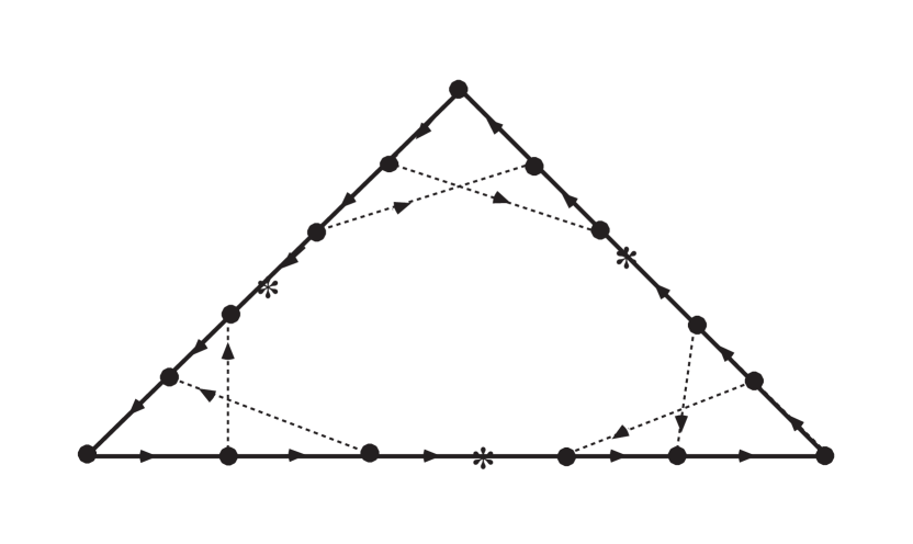
Figure 6: The graph representing a term obtained by pole decomposition. This graph separates into three disjoint parts when one cuts the three $*$ segments.

Consider first the case where all $r_{i}\neq 0$. In this case the Landau equations are equivalent to the Landau equations that arise from using the k-space variables, instead of the $(r,\Omega)$ variables. Then the Landau equations associated with the function represented by the graph shown in Fig. 6 can be expressed in a simple geometric form: these equations are equivalent to the existence of a “Landau diagram” (a diagram in four–dimensional space) that has the form shown in ^fig7).

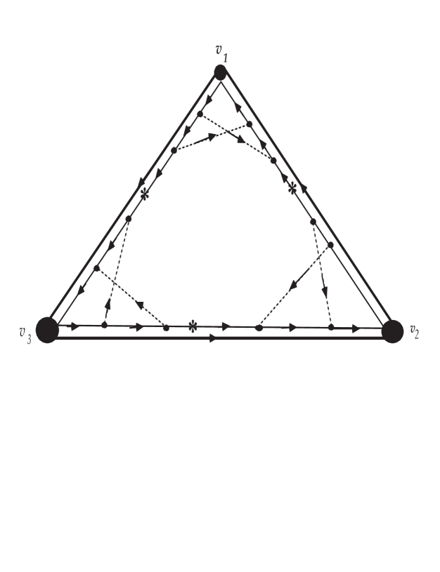
Figure 7: The Landau diagram associated with the graph of Fig. 6. We distinguish ‘Landau diagrams’ from ‘graphs: the former are geometric, the latter topological.

This Landau diagram is a diagram in four-dimensional space (thought of as spacetime), and each segment of the diagram represents a four vector. The rules are these:

1. Each directed photon line segment $i$ represents the vector

   $$V_{i}=\alpha_{i}k_{i},$$

   where $k_{i}$ is the momentum flowing along segment $i$ of the graph in the direction of the arrow, and $\alpha_{i}\geq 0$.

2. Each directed charged-particle segment $j$ corresponding to a pole-residue factor $f_{j}$ represents the vector

   $$V_{j}=\beta_{js}\Sigma_{j},$$

   where $\sum_{j}$ is the momentum flowing along segment $j$ of the graph in the direction of the arrow on it, and

   $$\sigma_{js}\beta_{js}=\alpha_{j}\geq 0,$$

   where the sign $\sigma_{js}$ is defined below (3).

3. Each directed charged-particle line segment $s$ corresponding to a pole denominator $(\sum^{2}_{s}-m^{2}+i0)$ is represented by a star (asterisk) line segment $s$, and it represents the vector.

   $$V^{\prime}_{s}=\alpha^{\prime}_{s}\Sigma_{s}\ \ \ \ \ ,$$

   where $\sum_{s}$ is the momentum flowing along $*$ line segment $s$ of the graph in the direction shown, and

   $$\alpha^{\prime}_{s}=\alpha_{s}-\sum_{j\epsilon J(s)}\beta_{js}.$$

   Here $\alpha_{s}$ is the Landau parameter $\alpha$ corresponding to the function $f_{s}=\sum^{2}_{s}-m^{2}+i0$, and for each side $s$ the set $J(s)$ is the set of indices $j$ that label the pole-residue denominators that are associated with side s of the triangle graph.

4. Three line segments appear in the Landau diagram that are not images of segments that appear in the graph. They are the three direct line segments that directly connect pairs of vertices from the set $\{v_{1},v_{2},v_{3}\}$. The vector $V_{s}$ associated with the direct segment $s$ is

   $$V_{s}=\alpha_{s}\Sigma_{s}+\sum_{j\epsilon J(s)}\beta_{js}(\Sigma_{j}-\Sigma_{s}).$$

   It is equal to the sum of the vectors corresponding to the sequence of $*$ and non $*$ charged-particle line segments that connect the pair of vertices $v_{i}$ between which the direct line segment $s$ runs.

The $p$ loop equation is represented by the closed loop formed by the three direct line segments $V_{s}$ specified in (6f) The photon loop equation associated with the photon line carrying momentum $k_{i}$ is formed by adding to $\alpha_{i}k_{i}$ the sum of the vectors corresponding to the charged-particle segments needed to complete a closed loop in the diagram (See Appendix B). Thus the existence of a (nontrivial) solution of the Landau equations is equivalent to the existence of a (nonpoint) Landau diagram having the specified topological structure, with its line segments equal to the vectors specified in (6).

Although Figs. 6 and 7 represent a separable case the rules described above general: they cover all cases in which all $r_{i}$ are nonzero.

For each s we can use in the Landau diagram either $V^{\prime}_{s}$ or $V_{s}$. We shall henceforth use always $V_{s}$, the segment that directly connects a pair of vertices $v_{i}$, rather than $V^{\prime}_{s}$, and we shall place a star (asterisk) on each of these three direct line segments. These three direct line segments are geometrically more useful than the $V^{\prime}_{s}\/$’s because they display immediately the p loop equations, and also the relative locations of the three external vertices $v_{i}$, and because each one has only a single contribution, $\alpha_{s}\Sigma_{s}$, of well-defined sign and direction, in the limit $k_{i}\Rightarrow 0$, provided condition (8)(see below) holds.

We specify the way that photon loops pass through Landau diagrams: a photon loop shall pass through the star line $s$ of a Landau diagram (i.e., along the direct line segment $s$) if and only if the corresponding loop in the graph passes through the star line $s$ of the graph.

The positivity of the photon-line $\alpha_{i}$’s entails that each directed vector $\alpha_{i}k_{i}$ of Fig. 7 points in the positive (energy/time) direction (i.e., to the left) if the energy $k^{0}_{i}$ is positive, and in the negative direction (i.e., to the right) if the energy $k^{0}_{i}$ is negative. This fact entails that positive energy is carried by each nonzero ( length) photon line segment of Fig. 7 out of the vertex that stands on its right–hand end and into the vertex that stands on its left–hand end. This result is true independently of the direction in which the arrow points, or of the sign of the energy component $k_{i}^{0}$.

In the general separable case some of the non $*$ segments may have $\alpha_{j}=0$, and hence contract to points. Consequently several photons may emerge from, or enter into, a single vertex of the Landau diagram.

This geometric representation of the “Landau” equations holds only if all $r_{i}\neq 0$. If one or more $r_{i}=0$ then the diagram breaks into parts, as will be seen. We wish to show, by using these geometric conditions and the result (5), that the $\Omega_{i}$ contours can be distorted in such a way as to avoid simultaneosly all the singularities except those associated with the three $*$ line poles, one for each of the three sides $s$ of $G$, and those associated with the various end points $r_{i}=0$ and $r_{i}=1$. We shall treat the various cases separately.

3. Separable Case; All $r_{i}\neq 0$.

To prove this result for the separable case, and when all $r_{i}\neq 0$, let us consider any one of the three disjoint partial diagrams of non $*$ segments. Let $V$ be the set of vertices of this partial diagram that lie on an end of at least one photon line that is not contracted to a point. Let $V_{R}$ be any element of $V$ such that every nonzero-length photon line incident upon $V_{R}$ has its other end lying to the left of $V_{R}$. Let $V_{L}$ be any element of $V$ such that every nonzero-length photon line that is incident upon $V_{L}$ has its other end lying to the right of $V_{L}$. Then the total momentum $K$ carried into either $V_{R}$ or $V_{L}$ by all photons incident upon it satisfies $K\neq 0$ and $K^{2}\geq 0$: these properties follow from the fact that each photon line of nonzero length incident upon $V_{R}$ must carry a light-cone-directed momentum-energy with positive energy out of $V_{R}$, and each photon line of nonzero length incident upon $V_{L}$ must carry a light-cone-directed momentum-energy with positive energy into $V_{L}$. However, one cannot satisfy $2pK+K^{2}=0$ with $p\simeq p_{1},p_{2}$ or $p_{3}$, and with a small $K\neq 0$ satisfying $K^{2}\geq 0$. Consequently the charged–particle line segments of the partial Landau diagram lying on the outer extremities of the two charged particle lines must contract to points, by virtue of (4a): the associated Landau parameter $\alpha_{i}$ must vanish. Recursive use of this fact entails that all of the lines in this partial diagram must contract to a single point.

The existence of zero–length photon lines whose ends do not lie in $V$ does not disturb this argument, provided self–energy parts are excluded.

This result, that each non $*$ line contracts to a point, means that every entry in every $\Omega_{i}$ loop equation vanishes. Under this condition the lemma expressed by Eq. (5) shows that every $\Omega_{i}$ contour can be distorted away from every $\Omega_{i}$–dependent singularity.

We next show that this result continues to hold when some or all of the $r_{i}$ vanish.

4. Separable Case; Some $r_{i}=0$

Let us first consider the simple example shown in ^fig8).

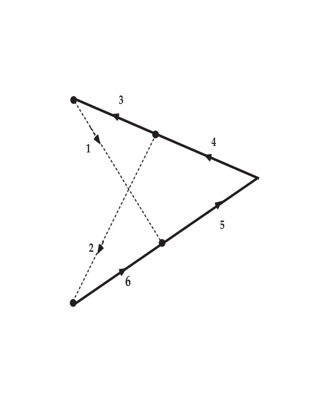
Figure 8: Part of the diagram of Fig. 7.

The Landau matrix for the diagram of Fig. 8 is shown in Fig. 9.

$$\begin{array}[]{lcc}f_{j}&{d\Omega_{1}}&{d\Omega_{2}}\cr\hline\cr&&\cr\Omega^{2}_{1}&\Omega_{1}&0\cr&&\cr\Omega^{2}_{2}&0&\Omega_{2}\cr&&\cr 2p_{1}\Omega_{1}+r_{1}\Omega^{2}_{1}&p_{1}+r_{1}\Omega_{1}&0\cr&&\cr 2p_{1}(\Omega_{1}+r_{2}\Omega_{2})+r_{1}(\Omega_{1}+r_{2}\Omega_{2})^{2}&p_{1}+r_{1}\Omega_{1}+r_{1}r_{2}\Omega_{2}&r_{2}(p_{1}+r_{1}\Omega_{1}+r_{1}r_{2}\Omega_{2})\cr&&\cr 2p_{2}(\Omega_{1}+r_{2}\Omega_{2})+r_{1}(\Omega_{1}+r_{2}\Omega_{2})^{2}&p_{2}+r_{1}\Omega_{1}+r_{1}r_{2}\Omega_{2}&r_{2}(p_{1}+r_{1}\Omega_{1}+r_{1}r_{2}\Omega_{2})\cr&&\cr 2p_{2}\Omega_{2}+r_{1}r_{2}\Omega_{2}^{2}&0&p_{2}+r_{1}r_{2}\Omega_{2}\cr\end{array}$$

Figure 9: The Landau matrix corresponding to the diagram of Fig. 8. The rows corresponding to the conditions $\Omega_{j}\widetilde{\Omega}_{j}=1$ have been removed, by using the argument given in Appendix A.

If $r_{1}\neq 0\neq r_{2}$ then one can multiply the $\Omega^{2}_{1}$ row by $r_{1}$, multiply the $\Omega^{2}_{2}$ row by $r_{1}r^{2}_{2}$, multiply the last row by $r_{2}$, and divide the $d\Omega_{2}$ column by $r_{2}$. This brings the matrix into an equivalent one in which $r_{1}$ and $r_{2}$ occur only in the combinations $k_{1}=r_{1}\Omega_{1}$ and $k_{2}=r_{1}r_{2}\Omega_{2}$: this is the equivalent $k$ form that was previously used for the case $r_{1}\neq 0\neq r_{2}$.

If $r_{1}=0$ and $r_{2}\neq 0$ then one can perform the same transformations involving $r_{2}$, and bring the equations to the same form as before, except that the vector associated with the photon line segment 1 is now $\alpha_{1}\Omega_{1}$ instead of $\alpha_{1}k_{1}$, and the vector associated with the photon line segment 2 is now $\alpha_{2}r_{2}\Omega_{2}$ instead of $\alpha_{2}k_{2}$. The vectors $r_{1}\Omega_{1}$ and $r_{1}r_{2}\Omega_{2}$ that occur summed with $p_{1}$ or $p_{2}$ become zero. Thus the situation is geometrically essentially the same as in the case $r_{1}\neq 0\neq r_{2}$, though slightly simpler: the small additions $k_{1}$ and $k_{2}$ to the vectors $p_{1}$ and $p_{2}$ now drop out. The important point is that the critical denominators $2pK+K^{2}$ of the earlier argument now take the form $2p\Omega$, with $\Omega^{2}\geq 0$ and $\Omega\neq 0$. Such a product cannot vanish. Thus the earlier $r_{i}\neq 0$ argument goes through virtually unchanged.

If $r_{1}\neq 0$ and $r_{2}=0$ then the $\Omega_{1}$ and $\Omega_{2}$ loop equations can be considered separately. The earlier $r_{i}\neq 0$ argument of section 3 can be applied to the first part alone, and it shows that each line segment on the $\Omega_{1}$ loop must contract to a point. Next the $\Omega_{2}$ equation can be considered alone, with each segment along which the $\Omega_{1}$ loop flows contracted to a point. Then the earlier $r_{1}=0$ arguments can be applied now to this $\Omega_{2}$ part of the diagram (with $r_{2}$ in place of $r_{1}$): it shows that each of the segments along which $\Omega_{2}$ flows also must contract to a point: the corresponding $\alpha_{j}$ must be zero.

The case $r_{1}=r_{2}=0$ is not much different from the case just treated: $r_{1}$ enters Fig. 9 only in an unimportant way.

The generalization of this argument from the case of Fig. 9 to the general separable case is straightforward. Let $r_{g}$ be the first vanishing element of the ordered set $r_{1},r_{2},...,r_{n}$. Then the set of $\Omega$ columns of the Landau matrix separates into one part involving only the $\Omega_{i}$ columns for $i<g$, and a second part involving only the $\Omega_{i}$ columns for $i\geq g$. For the first part of this matrix the argument given above for the case with all $r_{i}\neq 0$ holds, and it entails that every line segment in this part must contract to a point. With all of the rows corresponding to these contracted segments omitted one may apply the $r_{1}=0$ argument (with $r_{g}$ in place of $r_{1}$) to the part $i\geq g$, and proceed iteratively. This arguments leads to conclusion that the only solution to all of the $\Omega_{i}$ loop equations is the trivial one where every entry in every $\Omega$ column is zero. Hence the lemma expressed by Eq. (5) ensures that each $\Omega_{i}$ contour can be distorted away from all of its singularities, in the general separable case.

As one moves from the domain where all $r_{i}>0$ to the various boundary points where some $r_{i}=0$   two kinds of changes can occur. Certain conditions that particular vectors $\Omega_{j}$ be in the upper-half plane with respect to a variable like $(p_{1}+r_{1}\Omega_{1}+r_{1}r_{2}\Omega_{2})\cdot\Omega_{j}$ becomes slightly simplified when an $r_{i}$ becomes zero. Since the different conditions of this kind correspond to vectors $p_{1},p_{2}$, and $p_{3}$ that are well separated, the passage to a point $r_{i}=0$ causes no discontinuous change in the set of vectors that satisfy such conditions. The second kind of change is that some contributions to particular $d\Omega_{j}$’s may suddenly drop out if some $r_{i}$ vanishes. (See Fig. 9 with $r_{2}=0$). These changes at the boundary points of the region $r_{i}\geq 0$ do not entail any discontinuity in the distortion of the $\Omega$ contours on the boundary. The possibility of using a distortion in $\Omega$ space that is everywhere continuous in $(r,\Omega)$ follows from the continuousness of the gradients of the functions $f_{i}(r,\Omega)$, and the fact that at every point in the domain of integration the set of gradients of the set of vanishing $f_{i}$ form a convex set: the Landau equations cannot be satisfied.

5. Nonseparable Case; All $r_{i}\neq 0.$

We consider next the functions represented by graphs such that the cutting of the three $*$ segments does not separate the graph into three disjoint parts. The same result about distortions of $\Omega_{i}$ contours can be obtained also for these functions.

To obtain this result we consider first, as before, the case in which all $r_{i}\neq 0$. Then we may use the $k$ form of the Landau equations given in (6).

The argument proceeds as before, by making use of the vertices $V_{R}$ and $V_{L}$. No such vertex can join together two pole-residue segments $j$ of nonzero length: it is impossible to satisfy both $2pK_{1}+K_{1}^{2}=0$ and $2pK_{2}+K^{2}_{2}=0$ if $K_{1}-K_{2}=K$ satisfies $K^{2}\geq 0$ and $K\neq 0$, and $K_{1}$ and $K_{2}$ are small compared to the timelike $p$. Likewise, neither $V_{R}$ nor $V_{L}$ can join a $*$ segment to a pole-residue segment $j$ with $\alpha_{j}\neq 0$: one cannot satisfy $2pK+K^{2}=(2p+K)K=0$ if $K^{2}\geq 0$ and $K\neq 0$, and $K$ is much smaller than the timelike $p$. Consequently each of the vertices $V_{R}$ and $V_{L}$ must be confined to the set of external vertices $v_{i}$:

$$\{V_{R},V_{L}\}\subset\{v_{1},v_{2},v_{3}\}.$$

In the nonseparable case some of the signs $\sigma_{js}$ will be negative. Consequently some of the vectors corresponding to pole-residue factors $f_{j}$ will point in the ‘reversed’ direction, because their $\beta_{js}\/$’s, defined in (6c), are negative. There are also some (sometimes-compensating) reversals of the ways that certain photon loops run. These latter reversals arise because we have used, in the Landau diagrams, the three line segments that directly connect the pairs in $\{v_{1},v_{2},v_{3}\}$, rather than the images of the three star lines of the original $*$ graph. For example, the $*$ graph of Fig. 3c gives a Landau diagram of the form shown in ^fig10).

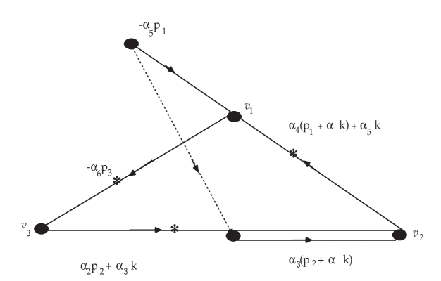
Figure 10: The Landau diagram corresponding to the $*$ graph (c) of Fig. 3. This diagram represents the equations obtained from Fig. 6c, with $f_{1}$ multiplied by $r^{2}$, $f_{3}$ and $f_{4}$ multiplied by $r$, and $r\Omega$ replaced by $k$. These changes recover the $k$ form of the equations. The backward orientation of the vector $\alpha_{5}p_{1}$ arises from the negative sign of $\sigma_{51}$. However, this vector is oriented against the direction of the photon loop. Consequently all contributions to this photon-loop equation proportional to any $p_{s}$ have the form $\alpha_{j}p_{s}$: the two reversals of the line segment $j=5$ compensate for each other.

A second example is the function represented by the graph shown in ^fig11).

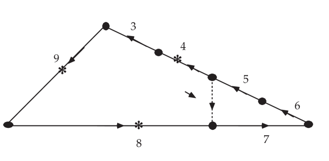
Figure 11: Figur A graph representing a term in the pole-decomposition expansion.

The functions $f_{j}$ and the Landau matrix corresponding to the function represented by the graph in Fig. 11 are shown in Fig. 12, for $\abs{k_{1}}>\abs{k_{2}}>0$

$$\begin{array}[]{lccc}{f_{j}}&{dk_{1}}&{dk_{2}}&{dp}\cr\hline\cr f_{1}=k^{2}_{1}&k_{1}&0&0\cr f_{2}=k^{2}_{2}&0&k_{2}&0\cr f_{3}=2p_{1}k_{1}+k^{2}_{1}&p_{1}+k_{1}&0&k_{1}\cr f_{4}=(p_{1}+k_{1})^{2}-m^{2}&p_{1}+k_{1}&0&p_{1}+k_{1}\cr f_{5}=2p_{1}k_{2}+2k_{1}k_{2}+k^{2}_{2}&k_{2}&p_{1}+k_{1}+k_{2}&k_{2}\cr f_{6}=2p_{1}(k_{1}-k_{2})+k^{2}_{1}-k^{2}_{2}&p_{1}+k_{1}&-(p_{1}+k_{2})&k_{1}-k_{2}\cr f_{7}=2p_{2}k_{2}+k_{2}^{2}&0&p_{2}+k_{2}&k_{2}\cr f_{8}=p^{2}_{2}-m^{2}&0&0&p_{2}\cr f_{9}=p^{2}_{3}-m^{2}&0&0&p_{3}\cr\end{array}$$

Figure 12: The Landau matrix for the function represented by the graph in Fig. 11, for $\abs{k_{1}}>\abs{k_{2}}>0$. The sign of $\sigma_{j1}$ is minus for $j=3$ and 6, and otherwise plus.

The Landau diagram corresponding to the Landau matrix in Fig. 12 is shown in ^fig13)

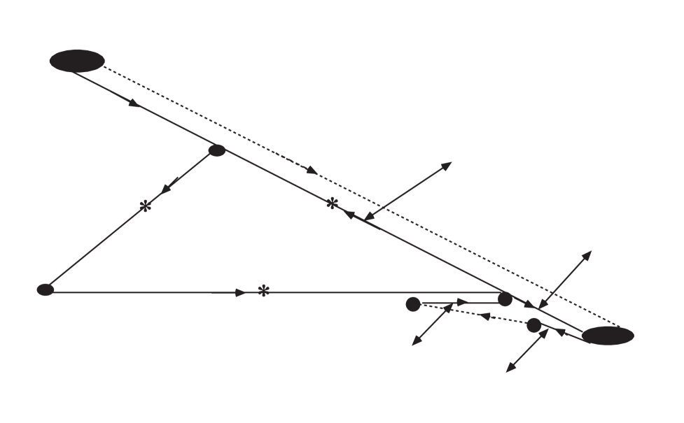
Figure 13: The ‘Landau diagram’ that represents the Landau equations associated with the Landau matrix shown in Fig. 12. This diagram is not a true Landau diagram, because, for example, the vector $\alpha_{i}k_{i}$ cannot be a light-cone vector. Moreover, condition (7) is not satisfied. Were it not for the non-negativity condition on $\alpha_{3}$ one could satisfy the Landau equations with $\alpha_{3}=-\alpha_{4}$, and $\alpha_{1}=\alpha_{2}=\alpha_{5}=\alpha_{6}=\alpha_{7}=0$.

The argument leading to (7) entails more than (7). It shows, in the present case where all $k_{i}\neq 0$, that each vertex of the diagram that does not lie in $\{v_{1},v_{2},v_{3}\}$ and that has at least one nonzero-length photon line segment incident upon it must have at least two nonzero-length photon lines incident upon it: each such vertex must lie on the right-hand end of at least one such photon line segment, and on the left-hand end of some other such photon line segment. Consequently, every nonzero-length photon line must lie on a ‘zig-zag’ path of photon lines that begins at a vertex in the set $\{v_{1},v_{2},v_{3}\}$, moves always to the left, and ends on another vertex in $\{v_{1},v_{2},v_{3}\}$: only in this way can the conditions $K^{2}\geq 0$ and $K\neq 0$ used in the derivation of (7) be overcome, if all $k_{i}$ are different from zero.

Consider, then, an example with vertices labelled as in ^fig14).

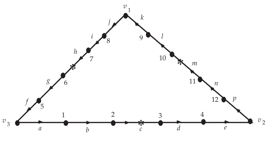
Figure 14: A triangle graph with photon vertices labelled by numbers, and charged–particle line segments labelled by letters. The segments $h,c,$ and $n$ are $*$ segments associated with the pole-decomposition formula $(0^{\prime})$. The photon lines have been suppressed.

Suppose $V_{L}=v_{3}$ and $V_{R}=v_{1}$ are the unique $V_{L}$ and $V_{R}$. Then some sequence of photon lines of nonzero length must join together to give a zig–zag path from $v_{1}$ to $v_{3}$. Three examples are shown in ^fig15.)

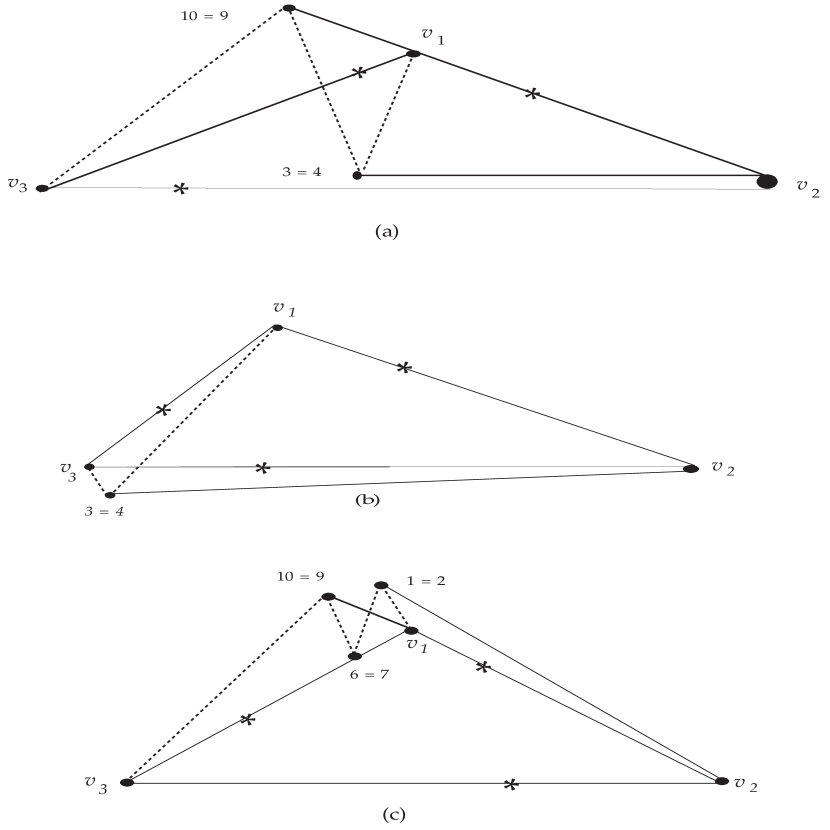
Figure 15: Three diagrams with zig–zag paths of photons connecting $v_{1}$ to $v_{3}$.

To analyse such diagrams we assume temporarily that for all pertinent solutions of the Landau equations

$$|\alpha_{j}|\leq|\alpha_{s}|B\ \hbox{for}\ j\epsilon J(s),$$

where $B$ is some fixed finite number. That is, we exclude temporarily the case where some $\alpha_{j}$ becomes unbounded, with the $\alpha_{s}$ bounded. Then as one lets the $\delta^{\prime}$ in (2) tend to zero the vector $V_{s}$ defined in (6f) and, for $j\in J(s)$, the vectors $V_{j}$ defined in (6b) all become increasingly parallel to $p_{s}$.

Consider then a sequence of bounds $\delta^{\prime}_{t}$, $t=1,2,...$, that tend to zero, and a corresponding sequence of solutions $S_{t}$ to the Landau equations in which:
1) $k_{i}\neq 0,\ i=1,...,n$;
2) $|k_{i}|\leq\delta^{\prime}_{t}/n,\ i=1,...,n$;
3) some $\alpha_{i}k_{i}\neq 0$; and
4) condition (8) holds.
If $q^{t}=(q^{t}_{1},q^{t}_{2},q^{t}_{3})$ is the vector $q=(q_{1},q_{2},q_{3})$ specified by $S_{t}$, then any accumulation point $\overline{q}$ of the set $\{q^{t}\}$ must be specified by a limiting diagram in which every charged-particle segment is parallel to one of the vectors $p_{s},s\in\{1,2,3\}$, and in which some zig-zag path of light-cone vectors runs leftward from a vertex $V_{R}$ of $\{v_{1},v_{2},v_{3}\}$ to a vertex $V_{L}$ of $\{v_{1},v_{2},v_{3}\}$, but carries zero momentum-energy. The limit point $\overline{q}$ must therefore lie on the Landau triangle diagram singularity surface $\varphi(q)=0$. However, the presence of the zig-zag photon line connecting two of the three vertices $v_{i}$ imposes an extra condition, which define a codimension-one submanifold of $\varphi(q)=0$. These submanifolds are finite in number (for any fixed graph $g$), and hence are nondense in the interior of $\varphi=0$. If a point $q\in\{\varphi=0\}$ lies at a nonzero distance from each of these submanifolds then no solution of the kind specified above can occur, and hence for some sufficiently small neighborhood $N$ of $q$, and for some sufficiently small $\delta^{\prime}$, any solution to the Landau equations for $q\in N$ satisfying $0<|k_{i}|\leq\delta^{\prime}/n$ for all $i$, and conditions 1) and 4), can have only zero-length photon lines: i.e., for all photon lines $i$

$$\alpha_{i}k_{i}=0\ \ .$$

We are interested here in the singularity structure at a general point on $\varphi=0$, rather than at special points where other singularity surfaces are relevant. Hence we may restrict our attention to a neighborhood $N$ in $\varphi=0$ where (9) holds.

Condition (9) says that every photon line segment $i$ must have zero length. This condition entails the stronger result that every segment on every photon loop $i$ in the Landau diagram must contract to a point.

To obtain this stronger result consider in order the loop equations corresponding to the sequence of variables $k_{1},...,k_{n}$, as defined in the formula $(0)$.

Consider first, then, the closed loop 1 in the Landau diagram. For each charged-particle segment on this loop the $k_{\ell}$ with smallest $\ell$ that flows along this loop 1 is $k_{1}$ itself. Consequently the orientations of all of the segments along this loop are unambiguously determined: for each $s\in\{1,2,3\}$ every contribution to the loop 1 that arises from a charged-particle segment on side $s$ adds to the loop equation a vector that is very close to a non-negative multiple of $p_{s}$, just as in Figs. 10 and 13. Use can be made here of the facts^8-11 that the triple of four-vectors $(v_{1},v_{2},v_{3})$ specified by the three external vertices $v_{i}$ constitute a normal to the Landau surface (in $q=(q_{1},q_{2},q_{3})$ space) associated with the diagram, and that this surface can be tangent to the triangle diagram Landau surface $\varphi(q)=0$ at a point $q$ only if the directions of the three vectors $V_{s}$ are the same as they are for the simple Landau diagram that corresponds to figure 4. Because we are staying away from exceptional points of lower dimension the three vectors $V_{s}$ must be parallel to the three vectors $p_{s}$. Alternatively, one can use the condition (8), and take $\delta^{\prime}$ sufficiently small, in order to deduce that $V_{s}$ is approximately equal to $\alpha_{s}p_{s}$.

Each photon loop passes along at most two sides s of the triangle. Hence, on any single photon loop in the Landau diagram, each charged-particle segment points approximately in the direction of one or the other of at most two of the three vectors $p_{s}$. (See Figs. 10 and 13.) Hence the contraction to a point, demanded by (9), of the remaining segment of the loop, namely $\alpha_{1}k_{1}$, forces every segment on loop 1 to contract to a point.

Consider next the loop 2. All segments along which $k_{1}$ runs have now been contracted out. Thus the $k_{\ell}$ with the smallest value of $\ell$ that flows along the surviving part of loop 2 is $k_{2}$ itself. Hence each segment on this loop also must contract to a point, by the same argument that was just used for loop 1. Proceeding step by step one finds that every segment on every photon loop must contract to a point.

In this nonseparable case with all $r_{i}\neq 0$ at least one photon line must pass along a star line. Hence at least one of the three star lines of the Landau diagram must also contract to a point. But then the other two sides of the triangle $(v_{1},v_{2},v_{3})$ must also contract to points, since, in accordance with the conditions imposed below Eq. (1), the three sides of the triangle connecting the three vertices $v_{i}$ are nonparallel. But then every segment of the Landau diagram is forced to a point, and thus there is no solution of the Landau equations, in this nonseparable case with all $r_{i}\neq 0$.

This conclusion was derived under the assumption (8). However, that assumption is not necessary. Suppose we normalized the solutions by the requiring that max $|v_{i}-v_{j}|=1$, and drop (8). Then the direction of $V_{s}$ is not constrained, but its Euclidean length is.

Consider, under these conditions, the sequence of loops $i$. A first part of loop 1 consists of either the zero, one, or two vectors $V_{s}$ that are included on the loop. Their directions are indeterminate, but their magnitudes are at most unity. In fact the magnitude of the sum of these segments is at most unity.

A second part of this closed loop is the segment corresponding to the photon 1 itself. The length of this segment is limited by the fact that any nonzero-length photon line segment must lie on a zig-zag path that runs between two of the vertices $v_{i}$, and is composed of leftward pointing light-cone vectors. Since the Euclidean distance between the endpoints of this zig-zag path is bounded by unity, the individual segments along this path are likewise bounded. Thus these first two parts of loop 1 are bounded.

The third and final part of loop 1 is the sum of the contribution of the segments $j$ associated with the pole-residue denominators $f_{j}$. All of these contributions to the loop are essentially of the form $\alpha_{j}p_{s}$, with all the $\alpha_{j}$’s positive, and $s$ ranging over either one or two of its three possible values. (See Figs. 10 and 13). We can impose the condition that at the points $q\in\{\varphi=0\}$ under consideration the three vectors $p_{s}$ are far from parallel. In this case the bound on the first two parts of the closed loop 1 imposes a comparable bound on the third part, and, in particular, a bound on the sum of the $\alpha_{j}$ corresponding to those segments $j$ that lie on loop 1.

We then turn to loop 2. Bounds are established as before for all parts of loop 2 that are not pole-residue segments $j$, and also for all pole-residue segments $j$ that lie on loop 1. Since the contributions from the pole-residue segments $j$ that lie on loop 2 but not loop 1 have the form $\alpha_{j}p_{s}$, with $\alpha_{j}\geq 0$, and with $s$ ranging over at most two of the three possible values, we can now establish upper bounds on the sum of these new $\alpha_{j}$’s. Proceeding in this way we establish bounds on all of the $\alpha_{j}\/$’s associated with all the pole-residue denominators $f_{j}$. Then for a sufficiently small $\delta^{\prime}$ we can ensure that, for each value of $s$, the contribution to $V_{s}$, specified by (6f), that arises from the photon momenta $k_{i}$ is small compared to this vector $V_{s}$ itself. This is the result that in the earlier argument was obtained from (8), which we therefore no longer need.

6. Nonseparable Case; Some $r_{i}=0$.

The results for the $k_{i}\neq 0$ case carry over to the general situation, provided the $(r,\Omega)$ variables are retained.

The argument for the case where some $r_{i}=0$ proceeds much as in the case of separable diagrams. Let $r_{g}$ be the first vanishing member of the ordered sequence $r_{1},r_{2},...,r_{n}$. Then the Landau matrix separates into two parts. The first consists of the $d\Omega_{i}$ columns for $i<g$, plus the $dp$ column; the second consists of the $d\Omega_{i}$ columns for $i\geq g$. By multiplying and dividing various rows and columns of the Landau matrix by appropriate nonzero factors $r_{i}$ ($i<g$) one can convert the $i<g$ part to the $k$ form, with all $k_{j}$ for $j\geq g$ set to zero. The $r_{i}\neq 0$ argument can then be applied to these $i<g$ Landau equations: they imply the vanishing of the $\alpha_{j}\/$’s corresponding to all segments $j$ of the Landau diagram along which run the photon loops $i$ with $i<g$.

The remaining columns, which give the $i\geq g$ part of the Landau equations, can be separated into sectors, where each sector begins with a column $d\Omega_{i}$ such that $r_{i}=0$, and is followed by the set of columns $d\Omega_{i+1},...,d\Omega_{i+h}$ such that $r_{i+1},...,r_{i+h}$ are all nonzero. These latter $r\/$’s can be changed to unity without altering the content of the Landau equations. We shall do this, purely for notational convenience.

The rows corresponding to the three pole denominators do not contribute to the $i\geq g$ equations because

$$\half{\partial\over\partial\Omega_{j}}[(p+r_{1}...r_{j}\Omega_{j}+...)^{2}-m^{2}]=0\ \hbox{for}\ j\geq g,$$

due to $r_{g}=0$.

One proceeds step-by-step, starting with the $i<g$ part, then considering the various individual sectors, in order of increasing values of $i$. The Landau equations for each one of the individual sectors can be expressed by a Landau diagram constructed in accordance with the rules (6), with, however, the following changes: (1), the three vectors $V_{s}$ corresponding to the three direct line segments $s$ are set to zero; (2), all the segments of the Landau diagrams that occur at earlier stages of the step-by-step process are contracted to points; and (3), the photon propagator contribution $\alpha_{i}k_{i}$ to each $d\Omega_{i}$ column that belongs to the sector in question is replaced by $\alpha_{i}\Omega_{i}$.

The Landau diagram corresponding to a sector S has a ‘spider’ form: it consists of a single central vertex $v$, which represents the three coincident vertices $v_{i}$, plus a web of segments sprouting out from $v$. All segments of the Landau diagrams corresponding to the previously considered sectors are contracted to the single point $v$, together with all of the segments that constitute the part $i<g$. All charged-particle segments of the Landau diagram along which run none of the photon loops that constitute S are also contracted to points.

The Landau diagram that corresponds to any individual sector S can be shown to contract to a point by using the arguments developed earlier: the argument involving $V_{R}$ and $V_{L}$ shows that no photon line of nonzero length can occur in the spider diagram, and then the step-by-step consideration of the photon loops $i$, in the order of increasing $i$, shows that each of these loops must contract in turn to a point.

We thus conclude that for every $j$ such that the Landau matrix element

$$L_{ij}\equiv\half\partial f_{j}/\partial\Omega_{i},$$

is non-zero for some $i$, $\alpha_{j}=0$. But then the lemma represented by Eq. (5) entails that one can distort the $\Omega_{i}$ contours in such a way as to move simultaneously into the upper-half plane of each of the residue-factor denominators $f_{j}$ and each of the photon-propagator denominators $(\Omega_{j})^{2}$. The only remaining singularities are the end-point singularities at $r_{i}=0$ and $r_{i}=1$, and the three Feynman denominators associated with the three $*$ lines of the $*$ graph $g$: for every other singularity surface $f_{j}=0$ there is some $\Omega_{i}$ such that $L_{ij}\neq 0$ for the corresponding $j$ and $i$. The consequences of the three $*$ line singularities in conjunction with the end-point singularities in the radial variables $r_{i}$ are dealt with in papers I and III.

Appendix A. Proof of the triviality of the contribution from the factor $\delta(\Omega_{j}\widetilde{\Omega}_{j}-1)$ to the Landau loop equations.

In discussing the singularities of the meromorphic parts in $\S 8$ we made full use of the fact that the row in the Landau matrix corresponding to $\Omega_{j}\widetilde{\Omega}_{j}-1$ reduces to zero under the closed loop conditions for $\Omega_{j}$-column, the $r_{j}$-column and the $r_{j+1}$-column. We give here a proof of this fact.

In view of the definition of the integral, the functions $f_{i}$ other than the various $\Omega^{2}_{j},\Omega_{j}\widetilde{\Omega}_{j}-1$  and $r_{j}$ have the following form (A.1) or (A.2), where $\epsilon_{m},$  and $\epsilon^{\prime}_{t}$ are each either $0$ or $+1$ or $-1$:

$$f_{i}=(p_{\ell}+\sum\epsilon_{m}r_{1}...r_{m}\Omega_{m})^{2}-m^{2}$$

$$\eqalignno{f_{i}&=2(p_{\ell}+\sum\epsilon_{m}r_{1}...r_{m}\Omega_{m})(\Omega_{s}+\sum\epsilon^{\prime}_{t}r_{s+1}...r_{t}\Omega_{t})\cr&+r_{1}...r_{s}(\Omega_{s}+\sum\epsilon^{\prime}_{t}r_{s+1}...r_{t}\Omega_{t})^{2}.&(A.2)\cr}$$

Let $H_{j}$ denote the first-order differential operator given by $\Omega_{j}{\partial\over\partial\Omega_{j}}-r_{j}{\partial\over\partial r_{j}}+r_{j+1}{\partial\over\partial r_{j+1}}$. Then the following equations hold:

$$\eqalignno{&H_{j}(p_{\ell}+\sum\epsilon_{m}r_{1}...r_{m}\Omega_{m})=0\ \ \hbox{ for any }\ j\ \hbox{and }\ell.&(A.3)\cr&H_{j}(\Omega_{s}+\sum\epsilon^{\prime}_{t}r_{s+1}...r_{t}\Omega_{t})&(A.4)\cr&=\Bigg{\{}\matrix{\Omega_{s}+\sum\epsilon^{\prime}_{t}r_{s+1}...r_{t}\Omega_{t}&\hbox{if}\ j=s\cr 0&\hbox{if}\ j\neq s},\cr&H_{j}(r_{1}...r_{s}(\Omega_{s}+\sum\epsilon^{\prime}_{t}r_{s+1}...r_{t}\Omega_{t})^{2})&(A.5)\cr&=\Bigg{\{}\matrix{r_{1}...r_{s}(\Omega_{s}+\sum\epsilon^{\prime}_{t}r_{s+1}...r_{t}\Omega_{t})^{2}&\hbox{if}\ j=s\cr 0&\hbox{if}\ j\neq s}\hbox{\hskip 36.135pt}.\cr}$$

Hence $H_{j}$ annihilates each $f_{i}$ of the form (A.1) and each $f_{i}$ of the form (A.2) with $s\neq j$, and it reproduces each $f_{i}$ of the form ( B.2) with $s=j$.

Since the $\Omega_{j}$-column etc. in the Landau matrix is given by $\partial f_{i}/\partial\Omega_{j}$ etc., this property of the operator $H_{j}$ entails, under the $\Omega_{j},r_{j}$, and $r_{j+1}$ closed-loop conditions, that

$$\eqalignno{0&=\Omega_{j}(\sum_{i}\alpha_{i}{\partial f_{i}\over\partial\Omega_{j}})-r_{j}(\sum_{i}\alpha_{i}{\partial f_{i}\over\partial r_{j}})+r_{j+1}(\sum_{i}\alpha_{i}{\partial f_{i}\over\partial r_{j+1}})\cr&=\sum_{i}\alpha_{i}H_{j}f_{i}\cr&=\sum_{i\epsilon I(j)}\alpha_{i}f_{i}+2a_{j}\Omega^{2}_{j}+2\beta_{j}\Omega_{j}\widetilde{\Omega}_{j}-\gamma_{j}r_{j}+\gamma_{j+1}r_{j+1},\cr}$$

where $I(j)$ denotes the set of indices $i$ such that $f_{i}$ is of the form (A.2) with $s=j$, and $a_{j},\beta_{j}$ and $\gamma_{j}$ denote the Landau parameters associated with $\Omega^{2}_{j},\ \Omega_{j}\widetilde{\Omega}_{j}-1$, and $r_{j}$, respectively. It follows from (4a) that all terms except for $\beta_{j}\Omega_{j}\widetilde{\Omega}_{j}=\beta_{j}$ on the right-hand side of (A.6) vanish. This entails the required fact, namely that the row corresponding to $\Omega_{j}\widetilde{\Omega}_{j}-1$ must have coefficient $\beta_{j}=0$ and hence give no net contribution to the Landau loop equations.

Appendix B. The Landau diagram corresponding to a term in the pole-decomposition expansion.

To confirm the geometric representation of the Landau equations described in connection with Eq.(6) recall first that the pole-residue denominators corresponding to non $*$ charged lines are

$$f_{j}=\sigma_{js}(\Sigma^{2}_{j}-\Sigma^{2}_{s})+i0,$$

where the sign $\sigma_{js}$ is defined below (3). For each side $s\epsilon\{1,2,3\}$ one may verify immediately that the contribution from the side $s$ of the triangle of direct lines $V_{s}$ is just the contribution to the $p$ loop equation arising from the charged-particle line segments that lie on side s of the original graph.

For the photon loop $\ell$ there is first a contribution $\alpha_{\ell}k_{\ell}$, and then the contributions corresponding to charge-particle line segments along which the loop flows. There are contributions of this latter kind only from segments corresponding to those (one or two) sides $s$ of the triangle along which the loop runs, and we can consider separately the contributions from each of those sides $s$.

There are three cases:

Case 1. The photon loop $\ell$ in the Feynman graph runs along the segment $j\epsilon J(s)$ but does not run along the $*$ segment lying on side $s$. In this case the contribution to the $\ell$ loop equation proportional to $\alpha_{j}$ is

$$\eqalignno{\alpha_{j}\half{\partial f_{j}\over\partial k_{\ell}}&=\sigma_{js}\alpha_{j}\half{\partial\over\partial k_{\ell}}(\Sigma^{2}_{j}-\Sigma^{2}_{s})\cr&=\beta_{js}\Sigma_{j}.&(B.2)\cr}$$

Case (2a). The loop $\ell$ of the Feynman graph flows along the $*$ segment of side $s$, but does not flow along the non $*$ segment $j$ lying on side $s$. Then the contribution to the $\ell$ loop equation proportional to $\alpha_{j}$ is

$$\eqalignno{\alpha_{j}\half{\partial f_{j}\over\partial k_{\ell}}&=\sigma_{js}\alpha_{j}\half{\partial\over\partial k_{\ell}}(\Sigma^{2}_{j}-\Sigma^{2}_{s})\cr&=\beta_{js}(-\Sigma_{s}).&(B.3)\cr}$$

Case (2b). The loop $\ell$ of the Feynman graph flows along the $*$ segment of side $s$ of the graph and also along the non $*$ segment $j\epsilon J(s)$. Then the contribution to the $\ell$ loop equation proportional to $\alpha_{j}$ is

$$\eqalignno{\alpha_{j}\half{\partial f_{j}\over\partial k_{\ell}}&=\beta_{js}\alpha_{j}\half{\partial\over\partial k_{\ell}}(\Sigma^{2}_{j}-\Sigma^{2}_{s})\cr&=\beta_{js}(\Sigma_{j}-\Sigma_{s}).&(B.4)\cr}$$

Notice that, according to (B.2), (B.3), and (B.4),there is, for each $j\epsilon J(s)$, a contribution $\beta_{js}\Sigma_{j}$ to the photon loop equation $\ell$ if and only if the loop $\ell$ in the graph passes along the segment $j$. There is also, for each $j\epsilon J(s)$, a contribution $-\beta_{js}\Sigma_{s}$ if and only if this loop passes along the star line $s$ in the graph. There is also a contribution $\alpha_{s}\Sigma_{s}$ if and only if this loop passes along the star line $s$ of the graph. These results are summarized by the rules (6).

References

1. T. Kawai and H.P. Stapp, Quantum Electrodynamics at Large Distances I: Extracting the Correspondence-Principle Part. Lawrence Berkeley Laboratory Report LBL 35971 (1994), Submitted to Phys. Rev.; See also H.P. Stapp, Phys. Rev. D28,1386 (1983)

2. H.P. Stapp, in Structural Analysis of Collision Amplitudes, ed. R. Balian and D. Iagolnitzer, North-Holland, New York, 1976, p.200 (Pham’s Theorem).

3. L.D. Landau, in Proc. Kiev Conference on High-Energy Physics (1959); Nuclear Physics 13 (1959) 181; N. Nakanishi, Prog. Theor. Phys. 22 (1959) 128.

4. R.J. Eden, P.V. Landshoff, D.I. Olive, and J.C. Polkinghorne, The Analytic S-matrix, Cambridge University Press, p.57 (1966);

5. T. Kawai and H.P. Stapp, in Algebraic Analysis, eds. M. Kashiwara and T. Kawai, Acad. Press (1988) Vol. I

6. T. Kawai and H.P. Stapp Publ. RIMS Kyoto Univ. 12 Suppl.155 (1977) Theorem 2.1.1

7. J. Coster and H.P. Stapp, J. Math Physics 11 (1970) 2743 (p. 2758)

8. C. Chandler and H.P. Stapp, J. Math. Phys. 10 (1969) 826.

9. D. Iagolnitzer and H. P. Stapp, Commun. Math. Phys. 14 (1969) 15.

10. H.P. Stapp, in Structural Analysis of Collision Amplitudes, ed. R. Balian and D. Iagolnitzer, North-Holland, New York, (1976).

11. D. Iagolnitzer, The S-matrix, North-Holland, (1978); Comm. Math. Phys. 41, 39 (1975); Comm. Math. Phys. 63, 49 (1978)