Contribution to “Bohmian Mechanics and Quantum Theory: An Appraisal,”
edited by J.T. Cushing, A. Fine, and S. Goldstein

Scattering Theory

from a Bohmian Perspective

Martin Daumer
Mathematisches Institut der Universität München,
Theresienstraße 39, 80333 München, Germany

Quantum mechanical scattering theory is a subject with a long and winding history. We shall pick out some of the most important concepts and ideas of scattering theory and look at them from the perspective of Bohmian mechanics: Bohmian mechanics, having real particle trajectories, provides an excellent basis for analyzing scattering phenomena.

1 A very brief historical sketch

We begin with a quote taken from Born 1926, shortly after Heisenberg 1925 had invented matrix mechanics and Schrödinger 1926 his wave mechanics:

Neither of these two conceptions appear satisfactory to me. I should like to attempt here to give a third interpretation and to test its utility on collision processes. In this attempt, I adhere to an observation of Einstein on the relationship of wave field and light quanta; he said, for example, that the waves are present only to show the corpuscular light quanta the way, and he spoke in the sense of a “ghost field”. This determines the probability that a light quantum …takes a certain path; …And here it is obvious to regard the de Broglie-Schrödinger waves as the ghost field or, better, “guiding field”.

I should therefore like to investigate experimentally the following idea: the guiding field, represented by a scalar function $\psi$ of the coordinates of all the particles involved and the time, propagates in accordance with Schrödinger’s differential equation. …The paths of these corpuscules are determined only to the extent that the laws of energy and momentum restrict them; otherwise, only a probability for a certain path is found.

and the

Closing remarks: On the basis of the above discussion, I should like to put forward the opinion that quantum mechanics permits not only the formulation and solution of the problem of stationary states, but also that of transition processes. In these circumstances Schrödinger’s version appears to do justice to the facts in by far the easiest manner; moreover, it permits the retention of the conventional ideas of space and time in which events take place in a completely normal manner. On the other hand, the proposed theory does not correspond to the requirement of the causal determinacy of the individual event. In my preliminary communication I stressed this indeterminacy quite particularly, since it appears to me in best agreement with the practice of the experimenter. But it is natural for him who will not be satisfied with this to remain unconverted and to assume that there are other parameters, not given in the theory, that determine the individual event. In classical mechanics these are the “phases” of the motion, i.e. the coordinates of the particles at a given instant. It appears to me a priori improbable that quantities corresponding to these phases can easily be introduced into the new theory, but Mr. Frenkel has told me that this may perhaps be the case. However this may be, this possibility would not alter anything relating the practical indeterminacy of collision processes, since it is in fact impossible to give the values of the phases; it must in fact lead to the same formulae as the “phaseless” theory proposed here.

Born 1926, translated in Ludwig 1968, p.224

Schrödinger 1926 had shown with his wave mechanics how to obtain the discrete energy levels of the hydrogen atom, by seeking stationary square integrable solutions of the Schrödinger equation (in units $\hbar=m=1$)

$$i\frac{\partial\psi_{t}({\bf x})}{\partial t}=-\frac{1}{2}\Delta\psi_{t}({\bf x})+V({\bf x})\psi_{t}({\bf x}).$$ (1)

What are called stationary states are solutions of the form $\psi_{t}({\bf x})=e^{-iEt}\psi({\bf x})$, where $\psi({\bf x})$ obeys the stationary Schrödinger equation

$$-\frac{1}{2}\Delta\psi({\bf x})+V({\bf x})\psi({\bf x})=E\psi({\bf x}),$$ (2)

which has square integrable solutions only for certain discrete energies $E_{n}<0$, in agreement with the experimental results. The physical meaning of the wave function was however unclear.

A description of a time-dependent scattering process was soon given by Max Born 1926, who explored the hypothesis that the wave function might be a “guiding field” for the motion of the electron. As a consequence of this hypothesis, Born is led in his paper to the “statistical interpretation” of the wave function: $\rho_{t}({\bf x})=|\psi_{t}({\bf x})|^{2}$ is the probability density for a particle to be at point ${\bf x}$ at time $t$. It follows from (1) that there is a conserved flux corresponding to this density, the quantum flux ${\bf j}^{\psi_{t}}({\bf x}):={\rm Im}\bigl{(}\psi_{t}^{*}({\bf x})\nabla\psi_{t}({\bf x})\bigr{)}$, which obeys the continuity equation

$$\frac{\partial|\psi_{t}({\bf x})|^{2}}{\partial t}+\nabla\cdot{\bf j}^{\psi_{t}}({\bf x})=0.$$ (3)

Born interpreted the quantum flux as a probability current of particles. His basic ansatz, sometimes called “naive” scattering theory (Reed, Simon 1979, p. 355), is to seek non-normalized solutions of the stationary Schrödinger equation (2) for positive energies $E=k^{2}/2$, which have the long-distance behavior

$$\psi({\bf x})\stackrel{{\scriptstyle x\to\infty}}{{\sim}}e^{i{\bf k}\cdot{\bf x}}+f(\theta,\phi)\frac{e^{ikx}}{x}.$$ (4)

$e^{i{\bf k}\cdot{\bf x}}$ is interpreted as the incoming plane wave and $f(\theta,\phi)\frac{e^{ikx}}{x}$ as the outgoing spherical wave with angular dependent density. The flux corresponding to the incoming wave is ${\bf k}$, such that the number of crossings per unit time and a unit surface orthogonal to ${\bf k}$ is $k:=|{\bf k}|$. The flux corresponding to the spherical wave is $\frac{{\bf x}}{x^{3}}k|f(\theta,\phi)|^{2}$ and is obviously purely radial. The number of crossings of the surface element $x^{2}d\Omega$ of a distant sphere in a direction specified by the angles $\theta,\phi$ per unit time divided by the number of incoming particles per unit time and unit surface is called “differential cross section,” and one finds

$$\frac{d\sigma}{d\Omega}=|f(\theta,\phi)|^{2}.$$ (5)

This description of a scattering process is however not convincing for simple reasons: there is no hint in the equations what the particles do which are responsible for the flux and how their motion is related to the wave function such that $\rho_{t}({\bf x})=|\psi_{t}({\bf x})|^{2}$ holds for all times. Moreover, the picture is entirely time-independent although a scattering process is certainly a process in space and time; stuff moves. The arguments leading to the formula (5) for the cross section “wouldn’t convince an educated first grader” (Goldberger, cited in Simon 1971, p 97).

From a physical point of view it might have seemed natural that a time-dependent justification of Born’s time-independent method was developed, involving a detailed analysis of the behavior of the wave function and its corresponding flux, but scattering theory proceeded along a different direction. (For the reasons why Born later abandoned the idea of a guiding field see e.g. Beller 1990.)

Heisenberg aimed at casting all in-principle-measurable quantities, such as energy levels and the cross section, into a single abstract object: the unitary $S$-matrix, or better, writing $S=e^{i\eta}$, into the self-adjoint “phase matrix” $\eta$ (Heisenberg 1946). $S$ should be the map from freely evolving “in”-states, which are controllable by an experimenter, to the freely evolving “out”-states, whose properties can be measured. Motivated by this idea Møller introduced the concept of “wave operators” (Møller 1946), the building blocks of the $S$-matrix: one expects that in a scattering process any wave function has a simple asymptotic behavior for large negative and positive times, where it should evolve almost freely with $e^{-iH_{0}t}$ ($H_{0}:=-\frac{1}{2}\Delta$). Hence there should be states $\phi_{+}$ and $\phi_{-}$ such that

$$\lim_{t\to\pm\infty}\|e^{-iHt}\psi-e^{-iH_{0}t}\phi_{\pm}\|_{2}=0,$$ (6)

where $\|\cdot\|_{2}$ is the norm in $L^{2}$. If the wave operators

$$\Omega_{\mp}={\mbox{\rm s-}}\lim_{t\to\pm\infty}e^{iHt}e^{-iH_{0}t}$$ (7)

(“${\mbox{\rm s-}}\lim$” denotes the strong limit) exist, then, if we now imagine that $\phi_{\pm}$ are given, obviously $\psi:=\Omega_{\mp}\phi_{\pm}$ obeys (6). (The strange sign convention is a tradition, see Reed, Simon 1979, p.17.)

The operators $\Omega_{\pm}$ should be unitary (we assume here that there are no bound states) such that $\Omega_{\pm}^{\dagger}=\Omega_{\pm}^{-1}$. The $S$-matrix can now be defined as $S=\Omega_{-}^{\dagger}\Omega_{+}$, because it maps freely evolving “in”-states onto “out”-states.

There has been a lot of work on the precise definition and properties of wave operators. We should mention here the concept of modified wave operators which was introduced (Dollard 1964) in order to bypass the problem, that the usual wave operators don’t exist for long range potentials such as the Coulomb potential. The program of “asymptotic completeness,” which aims at proving certain additional properties of the wave operators and the spectrum of the Hamiltonian, kept mathematicians and physicists busy for a long time, until recently this problem could be solved in great generality (Dereziński, Gerard 1993).

Interestingly enough, these achievements would not have been possible without the “renaissance” of geometrical ideas (Ruelle 1969, Enss 1978), namely by realizing that the wave packets evolve in space and time and are far away from the scattering center most of the time, instead of working with very abstract and complicated methods in momentum space (Faddeev 1965), where this simple geometrical picture easily gets lost.

Most of this work on the $S$-matrix, wave operators and asymptotic completeness is however not much concerned with the original question of scattering theory, the justification of the formula for the cross section (5) of the “naive” scattering theory, which was commonly used to do the actual numerical calculations. It is true that formulas for the differential cross section have been suggested from an analysis of $\langle{\bf k}^{\prime}|S|{\bf k}\rangle$, which was interpreted as the “probability density” to find the momentum eigenstate $|{\bf k}^{\prime}\rangle$ in the final state $S|{\bf k}\rangle$ (Lippmann and Schwinger 1950 used “adiabatic switching,” Gell-Mann and Goldberger 1953 Abelian limits), but these arguments were not much more convincing than the original argument to arrive at (5) (see also Reed, Simon 1979, p.356).

An exception is the work of Ikebe 1960, who rigorously established the physicist’s notation of expansions in continuum eigenfunctions (for “Ikebe”-potentials) and linked wave operators with solutions of the “Lippmann-Schwinger equation.” The time-dependent wave function (in physicists notation formally $\langle{\bf x}|e^{-iHt}|\psi\rangle=\int d^{3}ke^{-i\frac{k^{2}t}{2}}\langle{\bf x}\widetilde{|{\bf k}\rangle}\widetilde{\langle{\bf k}|}\psi\rangle)$ may be written as

$$\psi_{t}({\bf x})=(e^{-iHt}\psi)({\bf x})=(2\pi)^{-3/2}\int d^{3}ke^{-i\frac{k^{2}t}{2}}\phi({\bf x},{\bf k})\psi^{\#}({\bf k}),$$ (8)

where the “generalized eigenfunctions” $\phi({\bf x},{\bf k})$ are solutions of the Lippmann-Schwinger equation

$$\phi({\bf x},{\bf k})=e^{i{\bf k}\cdot{\bf x}}-\frac{1}{2\pi}\int d^{3}y\frac{e^{-i{k|{\bf x}-{\bf y}|}}}{|{\bf x}-{\bf y}|}V({\bf y})\phi({\bf y},{\bf k}).$$ (9)

Here $\psi^{\#}({\bf k}):=(2\pi)^{-3/2}\int d^{3}x\phi^{*}({\bf x},{\bf k})\psi({\bf x})$ is the “generalized Fourier transform” of $\psi$ and is connected with the wave operators by $(\widehat{\Omega_{-}^{\dagger}\psi})({\bf k})=\psi^{\#}({\bf k})$, where $\widehat{\ }$ denotes the usual Fourier transform. (There is another set of eigenfunctions corresponding to $\Omega_{+}$ which are in fact the ones most frequently used.) The solutions of the Lippmann-Schwinger equation are also solutions of the stationary Schrödinger equation with the asymptotic behavior as in (4) (the ones for $\Omega_{+}$) such that the differential cross section may be read off their long distance asymptotics as in (5). At least one could now find the formula (5) of the “naive” scattering theory somewhere in an appropriate expansion of the time-dependent wave function.

Another exception is the work of Dollard 1969. Dollard suggested to use the probability to find a particle in the far future in a given cone $C\subset\mathchoice{\hbox{${\rm I}\!{\rm R}$}}{\hbox{${\rm I}\!{\rm R}$}}{\hbox{$\scriptstyle{\rm I}\!{\rm R}$}}{\hbox{$\scriptscriptstyle{\rm I}\!{\rm R}$}}^{3}$ as a natural time-dependent definition of the cross section. Dollard’s “scattering-into-cones-theorem” relates this probability to the wave operators:

$$\lim_{t\to\infty}\int_{C}d^{3}x|\psi_{t}({\bf x})|^{2}=\int_{C}d^{3}v|\widehat{\Omega_{-}^{\dagger}\psi}({\bf v})|^{2}.$$ (10)

The scattering-into-cones-theorem has come to be regarded as the fundamental result from which the differential cross section ought to be derived (e.g. Reed, Simon 1979, p.356, and Enss, Simon 1980).

Dollard’s approach was however criticized by Combes, Newton and Shtokhamer 1975. They observe that the experimental relevance of the scattering-into-cones-theorem rests on the connection of the probability of finding the particle in the far future in a cone with the probability that the particle has, at some time, crossed a given distant surface subtended by the cone. Heuristically, the last probability should be given by integrating the quantum mechanical flux over the total time interval and this surface. (The flux is often used that way in textbooks.) Combes, Newton and Shtokhamer hence conjecture the “flux-across-surfaces-theorem”

$$\lim_{R\to\infty}\int_{0}^{\infty}dt\int_{C\cap{\partial B_{R}}}{\bf j}^{\psi_{t}}\cdot{\bf n}d\sigma=\int_{C}d^{3}v|\widehat{\Omega_{-}^{\dagger}\psi}({\bf v})|^{2},$$ (11)

where $B_{R}$ is the ball with radius $R$ and outward normal ${\bf n}$. There exists no proof of this theorem. Even the “free flux-across-surfaces-theorem ” for freely evolving $\psi_{t}$,

$$\lim_{R\to\infty}\int_{0}^{\infty}dt\int_{C\cap{\partial B_{R}}}{\bf j}^{\psi_{t}}\cdot{\bf n}d\sigma=\int_{C}d^{3}v|\hat{\psi}({\bf v})|^{2}$$ (12)

which should be physically good enough, because the scattered wave packet is expected to move almost freely after the scattering is essentially completed, has not been proven.

This is certainly strange because the physical importance of (11) and (12) for scattering theory is obvious and the mathematical problem does not seem to be too hard. Perhaps it was the vagueness in the meaning attached to the flux which is responsible for this matter of fact. For example, the authors try to reformulate the problem in operator language and are faced with the problem that for general $L^{2}$-functions the current across a given surface may well be infinite. Instead of using smooth functions they use “smeared-out” surfaces and therefore fail to find a proof of the original theorem. Or, for example, they argue that

At large distances the scattering part of the wave function contains outgoing particles only. Therefore the particles cannot describe loops there and the flux can be measured by the interposition of counters on ${\partial B_{R}}$.

and seem to have in mind a picture very similar to Born’s original proposal (cf. the Born quote), also without giving a precise guiding law for the trajectories which would allow, for example, to check the “no-loop-conjecture.”

Next we want to show how the ideas of Combes, Newton and Shtokhamer arise naturally by analyzing a scattering process in the framework of Bohmian mechanics (Bell 1987, Bohm 1952, Bohm and Hiley 1993, Dürr, Goldstein and Zangh’ı 1992 and their essay in this volume, Holland 1993): in this theory particles move along trajectories determined by the quantum flux, controlling the expected number of particles crossings of surfaces. We will sketch the main ideas of the proof of (12) (for the complete proof see Daumer 1995) and indicate the extension to the interacting case. We shall see that the flux-across-surfaces-theorem in Bohmian mechanics is a relation between the flux across a distant surface and the asymptotic probability of outward crossings of the trajectories of this surface—obviously the quantity of interest for the scattering analysis of any mechanical theory of point particles.

2 Bohmian Mechanics

Bohmian mechanics does what not only Born found “a priori improbable,” namely it shows that the introduction of additional parameters into the theory, represented by the Schrödinger equation (1), which “determine the individual event” is easily possible (see the essay of Dürr, Goldstein and Zangh’ı): the integral curves of the velocity field

$${\bf v}^{\psi_{t}}({\bf x})=\frac{{\bf j}^{\psi_{t}}}{\rho_{t}}({\bf x})={\rm Im}\frac{\nabla\psi_{t}}{\psi_{t}}({\bf x})$$ (13)

which are solutions of

$$\frac{d}{dt}{{\bf x}}(t)={\bf v}^{\psi_{t}}({{\bf x}}(t)),$$ (14)

together with an initial position ${\bf x}_{0}$ determine the trajectory of the particle. (For a proof of the global existence of the solutions for general $N$-particle systems and a large class of potentials see the essay of Berndl.) The initial position is distributed according to the quantum equilibrium probability $\mathchoice{\hbox{${\rm I}\!{\rm P}$}}{\hbox{${\rm I}\!{\rm P}$}}{\hbox{$\scriptstyle{\rm I}\!{\rm P}$}}{\hbox{$\scriptscriptstyle{\rm I}\!{\rm P}$}}^{\psi}$ ($\psi$ is normalized) with density $\rho=|\psi|^{2}$ (for a justification of “quantum equilibrium” see Dürr, Goldstein and Zangh’ı 1992).

Thus, in Bohmian mechanics  a particle moves along a trajectory guided by the particle’s wave function. Hence, given $\psi_{t}$, the solutions ${{\bf x}}(t,{{\bf x}}_{0})$ of equation (14) are random trajectories, where the randomness comes from the $\mathchoice{\hbox{${\rm I}\!{\rm P}$}}{\hbox{${\rm I}\!{\rm P}$}}{\hbox{$\scriptstyle{\rm I}\!{\rm P}$}}{\hbox{$\scriptscriptstyle{\rm I}\!{\rm P}$}}^{\psi}$-distributed random initial position ${{\bf x}}_{0}$, $\psi$ being the initial wave function.

Consider now a region $G\subset\mathchoice{\hbox{${\rm I}\!{\rm R}$}}{\hbox{${\rm I}\!{\rm R}$}}{\hbox{$\scriptstyle{\rm I}\!{\rm R}$}}{\hbox{$\scriptscriptstyle{\rm I}\!{\rm R}$}}^{3}$ and let $N^{\Sigma,\Delta}$ be the number of crossings of ${\bf x}(t)$ of subsets $\Sigma\subset\partial G$ in time intervals $\Delta\subset[0,\infty)$. Splitting $N^{\Sigma,\Delta}=:N_{+}^{\Sigma,\Delta}+N_{-}^{\Sigma,\Delta}$, where $N_{+}^{\Sigma,\Delta}$ denotes the number of outward crossings and $N_{-}^{\Sigma,\Delta}$ the number of backward crossings of $\Sigma$ in $\Delta$, we define for the number of “signed crossings” $N_{s}^{\Sigma,\Delta}:=N_{+}^{\Sigma,\Delta}-N_{-}^{\Sigma,\Delta}.$ By the very meaning of the probability flux it is rather clear (and it can easily be computed, Berndl 1995), that the expectated value of these numbers of crossings in quantum equilibrium is given by integrals of the current, namely

$$\mathchoice{\hbox{${\rm I}\!{\rm E}$}}{\hbox{${\rm I}\!{\rm E}$}}{\hbox{$\scriptstyle{\rm I}\!{\rm E}$}}{\hbox{$\scriptscriptstyle{\rm I}\!{\rm E}$}}^{\psi}(N^{\Sigma,\Delta}) = \int_{\Delta}dt\int_{\Sigma}|{\bf j}^{\psi_{t}}\cdot{\bf n}|d\sigma\/\Bigl{(}=\int d^{3}x|\psi({\bf x})|^{2}N^{\Sigma,\Delta}({\bf x})\Bigr{)}$$ (15)

$$\mathchoice{\hbox{${\rm I}\!{\rm E}$}}{\hbox{${\rm I}\!{\rm E}$}}{\hbox{$\scriptstyle{\rm I}\!{\rm E}$}}{\hbox{$\scriptscriptstyle{\rm I}\!{\rm E}$}}^{\psi}(N_{s}^{\Sigma,\Delta}) = \int_{\Delta}dt\int_{\Sigma}{\bf j}^{\psi_{t}}\cdot{\bf n}d\sigma.$$ (16)

(This relation between the current and the expected number of crossings is also one of the fundamental insights used in the proof of global existence of solutions.)

3 Scattering analysis of Bohmian mechanics

We want to analyze the scattering regime of Bohmian mechanics, i.e. the asymptotic behavior of the distribution of crossings of the trajectories traversing some distant surface surrounding the scattering center (see also Daumer 1995).

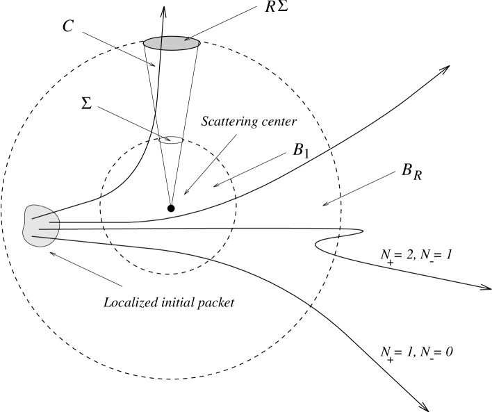
Figure 1: Possible trajectories of a particle starting in the wave packet localized in the ball $B_{R}$.

As surfaces we chose, for the sake of simplicity, spheres and we fix the notation illustrated in figure 1. (We may imagine the surface surrounding the scattering center or, more generally, simply an area in which the particle happens to be.)

We consider the random variables (functions of the paths) first exit time from $B_{R}$

$$t_{e}:=\inf\{t\geq 0|{\bf x}(t)\notin B_{R}\}$$ (17)

and the corresponding exit position

$${\bf x}_{e}={\bf x}(t_{e}).$$ (18)

Upon solving (14) and (1) the statistical distributions for $t_{e}$ and ${\bf x}_{e}$ can of course be calculated (see e.g. Leavens 1990 and his essay on the related problem of tunneling times). In general we should expect this to be a very hard task but it turns out that if ${\partial B_{R}}$ is at most crossed once by every trajectory—this is what we expect to happen asymptotically in the scattering regime—a very simple formula involving the current obtains.

The probability of the exit positions $\mathchoice{\hbox{${\rm I}\!{\rm P}$}}{\hbox{${\rm I}\!{\rm P}$}}{\hbox{$\scriptstyle{\rm I}\!{\rm P}$}}{\hbox{$\scriptscriptstyle{\rm I}\!{\rm P}$}}^{\psi}({\bf x}_{e}\in R\Sigma)$ should become “independent” of $R$ for large $R$ such that we may focus on the map $\sigma^{\psi}:{\cal B}(S^{2})\to\mathchoice{\hbox{${\rm I}\!{\rm R}$}}{\hbox{${\rm I}\!{\rm R}$}}{\hbox{$\scriptstyle{\rm I}\!{\rm R}$}}{\hbox{$\scriptscriptstyle{\rm I}\!{\rm R}$}}^{+}$ defined by

$$\sigma^{\psi}(\Sigma):=\lim_{R\to\infty}\mathchoice{\hbox{${\rm I}\!{\rm P}$}}{\hbox{${\rm I}\!{\rm P}$}}{\hbox{$\scriptstyle{\rm I}\!{\rm P}$}}{\hbox{$\scriptscriptstyle{\rm I}\!{\rm P}$}}^{\psi}({\bf x}_{e}\in R\Sigma)=\lim_{R\to\infty}\mathchoice{\hbox{${\rm I}\!{\rm P}$}}{\hbox{${\rm I}\!{\rm P}$}}{\hbox{$\scriptstyle{\rm I}\!{\rm P}$}}{\hbox{$\scriptscriptstyle{\rm I}\!{\rm P}$}}^{\psi}(\frac{{\bf x}_{e}}{x_{e}}\in\Sigma),$$ (19)

where $\frac{{\bf x}_{e}}{x_{e}}$ is the exit direction, which we expect to be a probability measure on the unit sphere (if eventually all trajectories go off to infinity, as they should.) This measure gives us the asymptotic probability of outward crossings of a distant surface, certainly the quantity of interest for the scattering analysis of any mechanical theory of point particles and it seems appropriate to define $\sigma^{\psi}$ in (19) as the cross section measure (see also the last section).

How can we find a handy expression for this probability?

With formula (15) we have already a formula for the expected number of crossings and the expected number of signed crossings of the surface $R\Sigma$ in the time interval $\Delta$. For large $R$ the sphere ${\partial B_{R}}$ should be crossed at most once, from the inside to the outside, such that the number of crossings equals the number of signed crossings, both being either 0 or 1, such that furthermore their expectation value equals the probability, that the particle has crossed the surface $R\Sigma$ at some time.

Hence, if there are asymptotically no backward crossings, i.e. if $\lim_{R\to\infty}\mathchoice{\hbox{${\rm I}\!{\rm E}$}}{\hbox{${\rm I}\!{\rm E}$}}{\hbox{$\scriptstyle{\rm I}\!{\rm E}$}}{\hbox{$\scriptscriptstyle{\rm I}\!{\rm E}$}}^{\psi}(N_{-}^{{\partial B_{R}},[0,\infty)})=0$, we find for the asymptotic probability that a trajectory crosses the surface $R\Sigma$ from the inside to the outside

$$\sigma(\Sigma)=\lim_{R\to\infty}\mathchoice{\hbox{${\rm I}\!{\rm P}$}}{\hbox{${\rm I}\!{\rm P}$}}{\hbox{$\scriptstyle{\rm I}\!{\rm P}$}}{\hbox{$\scriptscriptstyle{\rm I}\!{\rm P}$}}^{\psi}({\bf x}_{e}\in R\Sigma) = \lim_{R\to\infty}\int_{0}^{\infty}dt\int_{R\Sigma}{\bf j}^{\psi_{t}}\cdot{\bf n}d\sigma.$$ (20)

This is a very nice result, because it connects our (natural) definition of the cross section (19) with the quantity considered in the flux-across-surfaces-theorem (11).

Up to now the discussion leading to formula (20) has been completely general concerning the time evolution. Let us now process (20) further, taking the simplest case, namely free evolution. Our goal is to find a formula where the limit is taken.

The flux will contribute to the integral in (20) only for large times, because the packet has to travel a long time until it reaches the distant sphere ${\partial B_{R}}$ such that we may use the long-time asymptotics of the free evolution. We use the well-known formula (Reed, Simon 1975, p.59)

$$\psi_{t}({\bf x})=(e^{-iH_{0}t}\psi)({\bf x})=\int d^{3}y\frac{e^{i\frac{|{\bf x}-{\bf y}|^{2}}{2t}}}{(2\pi it)^{3/2}}\psi({\bf y})$$ (21)

and obtain with the splitting

$$\psi_{t}({\bf x})=\frac{e^{i\frac{x^{2}}{2t}}}{(it)^{3/2}}\hat{\psi}(\frac{{\bf x}}{t})+\frac{e^{i\frac{x^{2}}{2t}}}{(it)^{3/2}}\int\frac{d^{3}y}{(2\pi)^{3/2}}e^{-i\frac{{\bf x}\cdot{\bf y}}{t}}(e^{i\frac{y^{2}}{2t}}-1)\psi({\bf y}),$$ (22)

neglecting the second term, as $t\to\infty$

$$\psi_{t}({\bf x})\sim(it)^{-3/2}e^{i\frac{x^{2}}{2t}}\hat{\psi}(\frac{{\bf x}}{t}).$$ (23)

This asymptotics for scattering theory has since long been realized as important (e.g. Brenig and Haag 1959 and Dollard 1969, who proved that the asymptotics (23) holds in the $L_{2}$ sense). From (23) we find for $t\to\infty$

$${\bf j}^{\psi_{t}}({\bf x})={\mbox{\rm Im}}\/\psi_{t}^{*}({\bf x})\nabla\psi_{t}({\bf x})\approx\frac{{\bf x}}{t}t^{-3}|\hat{\psi}(\frac{{\bf x}}{t})|^{2},$$ (24)

and note, that the current and hence also the velocity is strictly radial for large times, i.e. parallel to the outward normal ${\bf n}$ of ${\partial B_{R}}$, reflecting our expectation that the expected value of backward crossings of ${\partial B_{R}}$ vanishes as $R\to\infty$.

Back to (20). Using the approximation (24) and substituting ${\bf v}:=\frac{{\bf x}}{t}$ we arrive at

$$\int_{0}^{\infty}dt\int_{R\Sigma}{\bf j}^{\psi_{t}}\cdot{\bf n}d\sigma \approx \int_{0}^{\infty}dt\int_{R\Sigma}t^{-3}|\hat{\psi}(\frac{{\bf x}}{t})|^{2}\frac{{\bf x}}{t}\cdot{\bf n}({\bf x})d\sigma$$ (25)

$$= \int_{0}^{\infty}dvv^{2}\int_{C}d\Omega|\hat{\psi}({\bf v})|^{2}=\int_{C}d^{3}v|\hat{\psi}({\bf v})|^{2}.$$

This heuristic argument for the free flux-across-surfaces-theorem (12) is so simple and intuitive that it is indeed strange that it does not appear in any primer on scattering theory!

Now let us turn to the interacting case. Using Ikebe’s eigenfunction expansion (8) and the relation of the generalized eigenfunctions with the wave operators we find that

$$\psi_{t}({\bf x})=(2\pi)^{-3/2}\int d^{3}ke^{-i\frac{k^{2}t}{2}}\phi({\bf x},{\bf k})\widehat{\Omega_{-}^{\dagger}\psi}({\bf k}).$$ (26)

The Lippmann-Schwinger equation (9) for $\phi({\bf x},{\bf k})$ allows us to split off the free evolution of $\Omega_{-}^{\dagger}\psi$ and we obtain

$$\psi_{t}({\bf x}) = e^{-iH_{0}t}\Omega_{-}^{\dagger}\psi$$ (27)

$$- (2\pi)^{-3/2}\int d^{3}ke^{-i\frac{k^{2}t}{2}}\widehat{\Omega_{-}^{\dagger}\psi}({\bf k})\Bigl{(}\frac{1}{2\pi}\int d^{3}y\frac{e^{-i{k|{\bf x}-{\bf y}|}}}{|{\bf x}-{\bf y}|}V({\bf y})\phi({\bf y},{\bf k})\Bigr{)}.$$

Now observe that the first term immediately gives with (25) the desired result

$$\lim_{R\to\infty}\int_{0}^{\infty}dt\int_{C\cap{\partial B_{R}}}{\bf j}^{\psi_{t}}\cdot{\bf n}d\sigma=\int_{C}d^{3}v|\widehat{\Omega_{-}^{\dagger}\psi}({\bf v})|^{2}.$$ (28)

The other terms which appear in the flux should not contribute for the following reason: they all contain the phase factor $e^{-i\frac{k^{2}t}{2}-ikx}$, where we used $e^{-ik|{\bf x}-{\bf y}|}\approx e^{-ikx}$ for $x$ far away from the range of the potential. This factor is rapidly oscillating for large $x$ and $t$ such that the $k$-integrals should decay fast enough in $x$ and $t$ to give no contribution to the flux across surfaces.

4 Morals

Let us recollect what we have achieved from our Bohmian perspective.

The analysis of the scattering regime of Bohmian mechanics suggests a natural definition of the cross section measure as the asymptotic probability distribution of the exit positions, formula (19). This is very similar to the definition of the cross section in classical mechanics (e.g. Reed, Simon 1979, p.15). The random distribution of impact parameters used in classical mechanics to define the cross section measure corresponds to the $|\psi|^{2}$ distribution of the initial positions of the particle. The “individual event” (cf. the Born quote at the beginning), that is the deflection of one particle in a certain direction, is indeed determined by the initial position. However, the initial positions are randomly distributed according to $|\psi|^{2}$ such that there is no way to control the individual event. What is relevant for a scattering experiment with a given wave function is the statistical distribution of these individual events and the flux-across-surfaces-theorem provides us with a formula for the asymptotic distribution.

Let us now examine how this formula may be connected with the usual operator formalism of quantum mechanics. The first step has already been done, by writing formula (19) in terms of wave operators instead of using the generalized eigenfunctions directly. (Existence of the wave operators and asymptotic completeness may appear as a by-product, once an eigenfunction expansion has been established (Green and Lanford 1960).) Note that formula (19) may be rewritten as

$$\sigma(\Sigma)=\int_{C}d^{3}v|\widehat{\Omega_{-}^{\dagger}\psi}({\bf v})|^{2}=(\psi,\Omega_{-}{\cal F}^{-1}P_{C}{\cal F}\Omega_{-}^{\dagger}\psi),$$ (29)

where $P_{C}$ denotes the projection operator on the cone $C$ and ${\cal F}$ is the unitary operator of the fourier transformation. The map $\Sigma\mapsto\Omega_{-}{\cal F}^{-1}P_{C}{\cal F}\Omega_{-}^{\dagger}$ is an explicit example of what is called a projection operator valued measure which corresponds to a unique self-adjoint operator by the spectral theorem. This particular example of escape statistics exemplifies the general situation, namely that operators as “observables” appear merely as computational tools in the phenomenology of certain types of experiments—those for which the statistics of the result are governed by a projection operator valued measure.

Now we come to the end of the closing remarks of the Born quote at the beginning. Is it true that any deterministic completion of quantum mechanics must lead to the same formulae for the cross section as Born’s formula?

Certainly not! Further assumptions would be required, e.g. the initial packet must be close to a plane wave, initially far away from the scattering center, in order to have a chance to arrive from formula (11) (or from Dollard’s formula (10)) at Born’s formula (5).

This is however not the strongest point we can make here, because Born’s formula is not really taken seriously as the fundamental formula for the cross section nowadays; but Dollard’s formula certainly is.

But what is the quantum mechanical prediction if we go further and do not want to make such strong idealizations, e.g. if we happen to place detectors around the scattering center which are not that far away? What are the predictions for the times and positions at which the detectors click? Dollard’s formula doesn’t apply here, because it is an asymptotic formula.

Maybe—after some reflection—one comes up with what seems a very natural candidate for the joint density of exit position and exit time, namely ${\bf j}^{\psi_{t}}({\bf x})\cdot{\bf n}({{\bf x}})d\sigma dt$. But further scrutinizing this answer within quantum mechanics should leave one uneasy. After all, this is a formula—a prediction—which is not at all a quantum mechanical prediction of the common type: ${\bf j}^{\psi_{t}}({\bf x})\cdot{\bf n}({{\bf x}})$ can well be negative and thus the formula makes sense only for (very) particular wave functions, for which ${\bf j}^{\psi_{t}}({\bf x})\cdot{\bf n}({{\bf x}})$ is positive. But what is then the right formula for all the other wave functions? Why is there such a simple formula for some wave functions?

In Bohmian mechanics there is no need to feel uneasy. $\mathchoice{\hbox{${\rm I}\!{\rm P}$}}{\hbox{${\rm I}\!{\rm P}$}}{\hbox{$\scriptstyle{\rm I}\!{\rm P}$}}{\hbox{$\scriptscriptstyle{\rm I}\!{\rm P}$}}^{\psi}(({{\bf x}}_{e},t_{e})\in(d\sigma,dt))$ is the probability that the particle exits at ${\bf x}_{e}$ at time $t_{e}$—and that can be calculated in the usual way for any wave function. For some wave functions it turns out (Daumer, Dürr, Goldstein and Zangh’ı 1994) to be indeed given by

$$\mathchoice{\hbox{${\rm I}\!{\rm P}$}}{\hbox{${\rm I}\!{\rm P}$}}{\hbox{$\scriptstyle{\rm I}\!{\rm P}$}}{\hbox{$\scriptscriptstyle{\rm I}\!{\rm P}$}}^{\psi}(({{\bf x}}_{e},t_{e})\in(d\sigma,dt))={\bf j}^{\psi_{t}}({\bf x})\cdot{\bf n}({{\bf x}})d\sigma dt,$$ (30)

for others it isn’t. That’s alright, isn’t it?

References

Bell, J.S. (1987), Speakable and Unspeakable in Quantum Mechanics, Cambridge University Press.

Beller, M. (1990), “Born’s probabilistic interpretation: a case study of ‘concepts in flux’,” Stud. Hist. Phil. Sci. 21, 563-588.

Bohm, D. (1952), “A suggested interpretation of the quantum theory in terms of “hidden” variables I, II,” Phys. Rev. 85, 166–179, 180–193.

Bohm, D., Hiley, B.J. (1993), The Undivided Universe: An Ontological Interpretation of Quantum Theory, Routledge & Kegan Paul, London.

Berndl, K. (1995), Zur Existenz der Dynamik in Bohmschen Systemen, PhD thesis, Mainz Verlag, Aachen.

Born, M. (1926), “Quantenmechanik der Stoßvorgänge,” Zeitschrift für Physik 38, 803–827, (translated in Ludwig (1968), p. 94-105).

Brenig, W., Haag, R. (1959), “General quantum theory of collision processes,” Fortschr. d. Phys. 7, 183–242, (translated in Ross (1963), 14–108).

Combes, J.-M., Newton, R.G., Shtokhamer, R. (1975), “Scattering into cones and flux across surfaces,” Phys. Rev. D 11, 366–372.

Daumer, M. (1995), Streutheorie aus der Sicht Bohmscher Mechanik, PhD thesis, Mainz Verlag, Aachen.

Daumer, M., Dürr, D., Goldstein, S., Zangh’ı, N. (1994), “Scattering and the role of operators in Bohmian mechanics,” 331–338, On Three Levels, M. Fannes, C. Maes, and A. Verbeure (eds.), NATO ASI series 324, Plenum, New York.

Daumer, M., Dürr, D., Goldstein, S., Zangh’ı, N. (1995), “On the flux across surfaces theorem”, in preparation.

Dereziński, J., Gerard, C. (1993), Asymptotic Completeness of $N$-particle Systems, Preprint, Erwin Schrödinger International Institute for Mathematical Physics, ESI 60.

Dollard, J.D. (1964), “Asymptotic convergence and the Coulomb interaction,” J. Math. Phys. 5, 729–738.

Dollard, J.D. (1969), “Scattering into cones I, Potential scattering,” Comm. Math. Phys. 12, 193–203.

Dürr, D., Goldstein, S., Zangh’ı, N. (1992), “Quantum equilibrium and the origin of absolute uncertainty,” J. Stat. Phys., 67, 843–907.

Enss, V., Simon, B., (1980), “Finite total cross section in nonrelativistic quantum mechanics,” Comm. Math. Phys. 76, 177-209.

Enss, V. (1978), “Asymptotic completeness for quantum mechanical potential scattering,” Comm. Math. Phys. 61, 285.

Faddeev, L. (1963), Mathematical aspects of the three-body problem in quantum scattering theory, (Steklov Math. Inst. 69), Israel Program for Scientific Translation.

Gell-Mann, M., Goldberger, (1953), “The formal theory of scattering,” Phys. Rev. 91, 298–408.

Green, T.A., Lanford III, O.E. (1960), J. Math. Phys. 1, 139.

Heisenberg, W. (1925), “Über die quantentheoretische Umdeutung kinematischer und mechanischer Beziehungen,” Z. f. Physik 33, 879.

Heisenberg, W. (1946), “Der mathematische Rahmen der Quantentheorie der Wellenfelder,” Z. f. Naturforschung 1, 608–622.

Holland, P. (1993), The quantum theory of motion, Cambridge University press.

Ikebe, T. (1960), “Eigenfunction expansions associated with the Schrödinger operator and their application to scattering theory,” Arch. Rational Mech. Anal. 5, 1–34.

Leavens, C.R. (1990), “Transmission, reflection and dwell times within Bohm’s causal interpretation of quantum mechanics,” Solid State Comm. 74, 923.

Lippmann, B., Schwinger, J. (1950), “Variational principles for scattering processes I,” Phys. Rev. 79, 469–480.

Ludwig, G. (1968), Wave mechanics, Pergamon Press, Oxford.

Møller, C. (1946), Kgl. Danske Videnskab. Selskab., Mat. -Fys. Medd. 23, 1, (reprinted in Ross (1963), p.109-154).

Reed, M, Simon, B. (1975), Methods of Modern Mathematical Physics II, Academic Press Inc., London.

Reed, M, Simon, B. (1979), Methods of Modern Mathematical Physics III, Academic Press Inc., London.

Ross, M. (1963), Quantum scattering theory, Indiana University Press, Bloomington.

Ruelle, D. (1969), “A remark on bound states in potential scattering theory,” Nuovo Cimento A 61, 655.

Schrödinger, E. (1926), “Quantisierung als Eigenwertproblem,” Ann. Phys. 79, 361–376, (translated in Ludwig (1968), p.94–105).

Simon, B. (1971), Quantum Mechanics for Hamiltonians defined as Quadratic Forms, Princeton University Press, Princeton, New Jersey.