Contribution to “Bohmian Mechanics and Quantum Theory: An Appraisal,”
edited by J.T. Cushing, A. Fine, and S. Goldstein

Global existence and uniqueness

of Bohmian trajectories

Karin Berndl
Mathematisches Institut der Universität München,
Theresienstraße 39, 80333 München, Germany

1 Introduction

Consider the equations of motion of Bohmian mechanics for a system of $N$ particles with masses $m_{1},...,m_{N}$ moving in physical space ${\rm I\!R}^{3}$: the wave function $\psi$ evolves according to Schrödinger’s equation

$$i\hbar\frac{\partial\psi_{t}(q)}{\partial t}=\left(-\sum_{k=1}^{N}\frac{{\hbar}^{2}}{2m_{k}}\Delta_{k}+V(q)\right)\psi_{t}(q),$$ (1)

and the configuration $Q=({\bf Q}_{1},\dots,{\bf Q}_{N})\in{\rm I\!R}^{3N}$, with ${\bf Q}_{k}\in{\rm I\!R}^{3}$ denoting the position of the $k$-th particle, evolves according to Bohm’s equation

$$\frac{dQ_{t}}{dt}=v^{\psi_{t}}(Q_{t}),$$ (2)

where the velocity field $v^{\psi}=({\bf v}^{\psi}_{1},\dots,{\bf v}^{\psi}_{N})$ is determined by the wave function $\psi$

$${\bf v}_{k}^{\psi}(q)=\frac{\hbar}{m_{k}}\mbox{Im}\frac{{\nabla}_{k}\psi(q)}{\psi(q)}$$ (3)

(Bohm 1952). This velocity field is regular on the subset of ${\rm I\!R}^{3N}$ where $\psi\neq 0$ and is differentiable. The question arises as to what happens if the configuration $Q_{t}$, when moving in accordance with (2) along integral curves of $v^{\psi_{t}}$, reaches at some time $\tau$ a singularity of $v^{\psi}$, for example a node of the wave function, i.e. a point where $\psi=0$. In general, the event of reaching a singularity of $v^{\psi}$ corresponds to a singularity of the motion: the velocity $dQ_{t}/dt$ becoming infinite, $Q_{t}$ being discontinuous, or even “exploding,” i.e. reaching infinity as $t\to\tau$. In some cases it may be possible to continue the Bohmian trajectory through a singularity of the velocity field, but in any case, Eqn. (2) is not defined at singularities of $v^{\psi}$, and the theory would have to be supplemented by a suitable prescription for how to extend the motion through a singularity, or which trajectories to avoid.

We should therefore consider the following problem—the initial value problem in Bohmian mechanics: For given initial values $\psi_{0}$ and $Q_{0}$ at a time $t_{0}$ (we shall put $t_{0}=0$), do there exist global unique solutions $(\psi_{t},Q_{t})$ of (1,2) such that $\psi_{t_{0}}=\psi_{0}$ and $Q_{t_{0}}=Q_{0}$? A positive answer to this question for all or at least for a suitable majority of initial conditions, or for a class of “physically relevant” initial conditions, is certainly important: the limits of global existence of solutions may hint at limits of validity of the theory.

Let us first give a simple explicit example where indeed some trajectories reach nodes of the wave function. Consider the one-dimensional harmonic oscillator (with $\hbar=m=\omega=1$), i.e, the potential $\displaystyle V(q)=q^{2}/2$, and take as the wave function a superposition of the ground state and the second excited state:

$$\psi_{t}(q)=e^{-q^{2}/2}\Bigl{(}1+(1-2q^{2})e^{-2it}\Bigr{)}e^{-it/2}.$$ (4)

This wave function leads to a velocity field $v^{\psi}$ which is an odd function of $q$ and periodic in time with period $\pi$. The Bohmian motion is therefore invariant under reflection $q\to-q$ and periodic in $t$ with period $\pi$: If $Q(t)$ is a solution of (2), then $-Q(t)$ is also a solution of (2), and $Q(t+\pi)=Q(t)$. The wave function $\psi$ has nodes at $(q,t)=(0,(n+1/2)\pi)$ and at $(q,t)=(\pm 1,n\pi)$ for all integers $n$. There are three trajectories which periodically run into nodes of $\psi$, see Figure 1. One of them, the constant $Q_{t}=0$ for $t\neq(n+1/2)\pi$, is a solution of (2) which runs with velocity 0 at times $t\to(n+1/2)\pi$ into nodes of $\psi$. The other two “node-crossing” trajectories (which are reflection images of each other) are singular at the nodes: for example, in the vicinity of the node at $q=1$, $t=0$ the trajectory running into it has the form $\displaystyle Q_{t}=(3t^{2}/4)^{1/3}+1$, i.e. it has infinite velocity at $t=0$.

In this example the trajectories may be continued through the nodes in an obvious and consistent way. This is an artifact of the low dimensionality: In fact, in $d=1$ dimension, $Q_{t}$ satisfies

$$\int_{-\infty}^{Q_{t}(q_{0})}|\psi_{t}(q)|^{2}\,dq=\int_{-\infty}^{q_{0}}|\psi_{0}(q)|^{2}\,dq,$$ (5)

employing the equivariance of the $|\psi_{t}|^{2}$-measure, i.e. that the density $\rho_{0}=|\psi_{0}|^{2}$ evolves under the Bohmian dynamics to $\rho_{t}=|\psi_{t}|^{2}$ (Dürr, Goldstein, Zanghì 1992a; see also Section 4), and the property that trajectories do not cross in configuration-space-time. Clearly, much less regularity of $\psi$ is needed for this definition of the motion of the Bohmian configuration—in particular, nodes of the wave function are no problem—and, if both definitions (2) and (5) are possible, they agree. However, a generalization of (5) to the physically most interesting case of $d=3N$-dimensional configuration space is not known. We shall turn now to the question of the existence of global unique solutions of the equations of motion of Bohmian mechanics, (1) and (2).

2 The Schrödinger equation

In Bohmian mechanics, the evolution of the wave function $\psi$ according to Schrödinger’s equation (1) is independent of the evolution of the actual particle configuration $Q$ according to the guiding equation (2), while for the integration of (2) we need $\psi$. Therefore, when solving the initial value problem, we may consider Schrödinger’s equation first.

The linear partial differential equation (1) is usually discussed in the framework of the Hilbert space ${\cal H}=L^{2}({\rm I\!R}^{3N})$ of square integrable functions, by viewing the Hamiltonian $\displaystyle\widetilde{H}=-\sum_{k=1}^{N}\frac{{\hbar}^{2}}{2m_{k}}\Delta_{k}+V(q)$ as the generator of the unitary group $U_{t}=e^{-iHt/\hbar}$ (Kato 1951, Reed and Simon 1975). Usually, boundary conditions on the wave function have to be specified in order to get a unique time evolution $(U_{t})_{t\in{\rm I\!R}}$. In more technical terms, one has to select a self-adjoint extension $H$ of the partial differential operator $\widetilde{H}$, which is a priori defined only on sufficiently smooth functions. As different self-adjoint extensions generate different time evolutions of the wave function, the choice of the right self-adjoint extension is a matter of physics. We shall comment on this in Section 4. Given $(U_{t})_{t\in{\rm I\!R}}$, for any initial $\psi_{0}\in{\cal H}$ we have a global unique wave function $\psi_{t}=U_{t}\psi_{0}$. This wave function, however, in general is not a genuine solution of Schrödinger’s equation: Generic $\psi_{0}\in{\cal H}$ are not smooth functions, and $\psi_{t}$ will not be differentiable, so that the differential equation (1) cannot be discussed. The standard procedure now is to forget about Schrödinger’s equation, and argue that all one is interested in is a unitary time evolution—or, even more abstractly, a unitary representation of the time translation group. This is, however, not sufficient for our approach. From the point of view of Bohmian mechanics, the wave function $\psi$ is a smooth field on configuration-space-time solving Schrödinger’s equation. To obtain this, we have to put suitable conditions on the initial wave function $\psi_{0}$. It turns out that a suitable subspace of ${\cal H}$ is given by the so-called $C^{\infty}$-vectors of the Hamiltonian $H$, $\displaystyle C^{\infty}(H)=\bigcap_{n=1}^{\infty}{\cal D}(H^{n})$. ${\cal D}(H^{n})$ denotes the domain of the $n$-th power of the Hamiltonian, i.e. the set of wave functions for which the expectation value of the $2n$-th power of $H$, the “energy,” is finite, $\displaystyle\int_{{\rm I\!R}^{3N}}(H^{n}\psi)^{2}\,dq=\langle\psi|H^{2n}\psi\rangle<\infty$.¹ $C^{\infty}(H)$ is a dense subset of ${\cal H}$, and invariant under the time evolution $U_{t}$. Eigenfunctions and wave packets are special $C^{\infty}$-vectors, so all wave functions usually considered in physics are included. It should not at all be regarded as a defect of Bohmian mechanics that it is not defined for all $\psi_{0}\in{\cal H}$: From the point of view of Bohmian mechanics, the Hilbert space $L^{2}({\rm I\!R}^{3N})$ is not the state space of the wave function, but a useful tool for the analysis of the theory. (In this context, see also the contributions of Dürr, Goldstein, Zanghì and Daumer to this volume.)

We have: For any $\psi_{0}\in C^{\infty}(H)$, $\psi_{t}=U_{t}\psi_{0}=e^{-itH/\hbar}\psi_{0}$ is a global smooth solution of Schrödinger’s equation on $\Omega\times{\rm I\!R}$, where $\Omega$ denotes the set where the potential is smooth. This result cannot be genuinely strengthened: the wave function cannot be expected to be regular at points where the potential is singular. For instance, the ground state eigenfunction of the Coulomb potential $V(q)=1/|q|$, $e^{-|q|}$, is not differentiable at the singularity of the potential at $q=0$. Important examples of potentials are the $N$-particle Coulomb interaction for particles with charges $e_{i}$

$$V_{\rm Coulomb}({\bf q}_{1},\dots,{\bf q}_{N})=\sum_{i=1}^{N}\sum_{j=i+1}^{N}\frac{e_{i}e_{j}}{|{\bf q}_{i}-{\bf q}_{j}|}$$

with $\displaystyle\Omega_{\rm Coulomb}={\rm I\!R}^{3N}\setminus\bigcup_{i=1}^{N}\bigcup_{j=i+1}^{N}\{{\bf q}_{i}={\bf q}_{j}\}$, and the $N$-electron atom

$$V_{\rm atom}({\bf q}_{1},\dots,{\bf q}_{N})=\sum_{i=1}^{N}\frac{e_{n}e_{i}}{|{\bf q}_{i}|}+\sum_{i=1}^{N}\sum_{j=i+1}^{N}\frac{e_{i}e_{j}}{|{\bf q}_{i}-{\bf q}_{j}|}$$

with $\displaystyle\Omega_{\rm atom}={\rm I\!R}^{3N}\setminus\Biggl{(}\bigcup_{i=1}^{N}\{{\bf q}_{i}=0\}\cup\bigcup_{i=1}^{N}\bigcup_{j=i+1}^{N}\{{\bf q}_{i}={\bf q}_{j}\}\Biggr{)},$ in the approximation that the nucleus with charge $e_{n}$ is at rest at the origin, acting like an external Coulomb field.

3 The Bohmian trajectories

With the wave function $\psi\in C^{\infty}(\Omega\times{\rm I\!R})$, the velocity field $v^{\psi}$ (3) can be formed on the set where the wave function $\psi\neq 0$. We shall call the set where the velocity field is regular ${\cal G}=(\Omega\times{\rm I\!R})\setminus{\cal N}$, where ${\cal N}$ is the (space-time) set of nodes of the wave function ${\cal N}=\{(q,t)\in\Omega\times{\rm I\!R}:\psi_{t}(q)=0\}$. On this set, the first order ordinary differential equation (2) is locally integrable. If we extend the solution as far as possible, we obtain for each initial value $q_{0}\in{\cal G}_{0}$, i.e. $(q_{0},0)\in{\cal G}$, a maximal solution $Q(t;q_{0})$ on a maximal time interval of existence $(\tau^{-}(q_{0}),\tau^{+}(q_{0}))$. The solution is called global if $\tau^{-}=-\infty$ and $\tau^{+}=+\infty$. In the introduction we have given an example showing that we cannot expect to have global solutions for all initial values $q_{0}$. But what indeed holds true is that for almost all initial configurations we have global unique solutions. “Almost all” here is with respect to the natural—the equivariant—measure $P^{\psi_{0}}$ on configuration space ${\rm I\!R}^{3N}$, that is the measure with the density $|\psi_{0}|^{2}$. We have proved that for a large class of potentials, including the N-particle Coulomb interaction with arbitrary masses and charges, as well as arbitrary positive potentials, $P^{\psi_{0}}(\tau^{+}=+\infty$ and $\tau^{-}=-\infty)=1$. In other words, for almost any initial point $Q_{0}$, the solution of the guiding equation (2) is global, i.e. nodes of the wave function or other singularities of the velocity field will not be reached in finite time, and the solution does not “explode,” i.e. reach infinity in finite time. (Cf. the example of Figure 1: the set of initial configurations for which the solution of (2) is not global consists of 3 points—certainly a set of $P^{\psi_{0}}$-measure 0—while for all the other initial values the solution is global.)

We shall comment on the proof—which is in fact quite intuitive—in the next section. (For the details, see Berndl, Dürr, Goldstein, Peruzzi, Zanghì 1995.) Despite the relative simplicity of the proof, the generality of the result is rather surprising. The analogous problem in Newtonian mechanics—global existence and uniqueness of solutions of the $N$-body problem for Newtonian gravity—is a classical problem of mathematical physics which has been investigated with a great variety of methods (Moser 1973, Diacu 1992), but for which the analogous result—global existence of solutions for Lebesgue-almost all initial values in the $N$-particle phase space ${\rm I\!R}^{6N}$—has not yet been established. In addition to the possibility of collision singularities, the $N$-body problem with $N>3$ yields marvelous scenarios of so-called pseudocollisions, where some particles, while oscillating wildly, reach infinity in finite time. Examples of such catastrophies have been constructed by Mather and McGehee 1975,² by Gerver 1991, and by Xia 1992. For special situations, such as for example an almost planar solar system with weakly eccentric planets, the KAM theorem furnishes among other things the existence of global solutions for a set of initial values of positive Lebesgue measure in phase space (cf. for example Arnold 1963). For the general case of the $N$-body problem with $N\geq 5$ it is still open whether for almost all initial values the solutions of Newtonian gravity are global or whether pseudocollisions occur on a set of positive measure.

The explanatory power of Newtonian mechanics rests largely on the analysis of specific solutions of the equations of motion, such as for example the planetary motion, or the gyroscope motion—physical situations where the bodies are modelled by fixed mass densities. The more ambitious program of Newtonian mechanics for a system composed of a huge number of point particles or rigid balls, for example the statistical gas theory, is difficult for two reasons. Firstly, to get global existence of solutions for almost all initial values—certainly a prerequisite of a statistical analysis—one has to deal for example with the problem of singular interactions in the case of point particles resp. multiple collisions in the case of rigid balls. Secondly, more interesting than equilibrium properties and much more difficult to analyse are the physical effects occuring in the transition from nonequilibrium to equilibrium.

In Bohmian mechanics, actual trajectories are interesting in some cases. However, to determine the equilibrium properties they are not needed. And in contrast to the situation in classical physics, we have the strongest empirical evidence that our world is in quantum equilibrium (Dürr, Goldstein, Zanghì 1992a and 1992b). Our theorem of global existence of Bohmian trajectories is thus exactly what is necessary and sufficient for a complete analysis of Bohmian mechanics. It provides the rigorous basis for the derivation of the quantum formalism as well as scattering theory from an equilibrium analysis of Bohmian mechanics. (These topics are described in the contributions of Dürr, Goldstein, Zanghì and Daumer to this volume.) In this sense, what we have proved is just that $|\psi|^{2}$ is an equivariant density for the Bohmian particle motion,

$$\rho_{0}=|\psi_{0}|^{2}\quad\Longrightarrow\quad\rho_{t}=|\psi_{t}|^{2}\quad\mbox{ for all }t\in{\rm I\!R}.$$ (6)

4 The quantum flux

The preceding sentence may have confused readers: Why isn’t the equivariance of the $|\psi_{t}|^{2}$-measure clear without an intricate examination of the global existence and uniqueness of solutions of Bohmian mechanics? Why doesn’t (6) follow immediately from a comparison of the continuity equation for an ensemble of configurations moving with velocity $v^{\psi}$ and having a density $\rho_{t}(q)$

$$\frac{\partial}{\partial t}\,\rho_{t}(q)\ +\ \sum_{k=1}^{N}\mbox{div}_{k}\,\bigl{(}{\bf v}^{\psi_{t}}_{k}(q)\,\rho_{t}(q)\bigr{)}\ =\ 0$$ (7)

with the “quantum continuity equation”

$$\frac{\partial}{\partial t}\,|\psi_{t}(q)|^{2}\ +\ \sum_{k=1}^{N}\mbox{div}_{k}\ {\bf j}^{\psi_{t}}_{k}(q)\ =\ 0,$$ (8)

noting that the quantum probability current $j^{\psi}=({\bf j}_{1}^{\psi},...,{\bf j}_{N}^{\psi})$ is given by

$${\bf j}_{k}^{\psi}\ =\ {\bf v}_{k}^{\psi}\,|\psi|^{2}\ =\ \frac{\hbar}{{m}_{k}}\,{\rm Im}\,({\psi}^{\ast}{\nabla}_{k}\psi)\ ?$$

The answer is that the continuity equation (7) expresses how an ensemble density $\rho_{0}$ evolves under the deterministic evolution of the trajectories, and holds therefore on just that set which is covered by the integral curves of $v^{\psi_{t}}$. We shall denote this set—the image set of the maximal solution $Q$—by ${\cal I}$:

$${\cal I}=\{(q,t)\in{\cal G}:\exists q_{0}\in{\cal G}_{0}\ \mbox{with}\ t\in(\tau^{-}(q_{0}),\tau^{+}(q_{0}))\ \mbox{and}\ q=Q_{t}(q_{0})\}.$$

Equation (8), on the other hand, is an identity for every $\psi_{t}$ which solves Schrödinger’s equation. Thus (6) holds on ${\cal I}$: $\rho_{t}(q)=|\psi_{t}(q)|^{2}$ for $(q,t)\in{\cal I}$. By putting $\rho_{t}(q)=0$ on the set which is not reached by the Bohmian trajectories $(\Omega\times{\rm I\!R})\setminus{\cal I}$, we obtain $\rho_{t}(q)\leq|\psi_{t}(q)|^{2}$ for $(q,t)\in\Omega\times{\rm I\!R}$. This insight is fundamental to the proof of global existence.

The second fundamental insight comes from the consideration of the configuration-space-time flux $J(q,t)=(v^{\psi_{t}}(q)\rho_{t}(q),\rho_{t}(q))$. To establish $P^{\psi_{0}}(\tau^{+}=+\infty$ and $\tau^{-}=-\infty)=1$, i.e. that for $P^{\psi_{0}}$-almost all initial configurations $q_{0}$ the maximal solution is global, we have to show that the solution will reach singularities of the velocity field or infinity in finite time at most for a set of initial configurations of $P^{\psi_{0}}$-measure zero. The probability of such a “bad event” is estimated with the help of the flux $J(q,t)$: For any hypersurface $\Sigma$ in configuration-space-time with local normal vector field $n(q,t)$ and surface area element $d\sigma$,

$$\int_{\Sigma}|J(q,t)\cdot n(q,t)|\,d\sigma$$

is the expected number of crossings of the hypersurface $\Sigma$ by the Bohmian trajectory and hence a bound for the probability of crossing $\Sigma$. We obtain

$$P^{\psi_{0}}(Q_{t}\mbox{ crosses }\Sigma)\leq\int_{\Sigma}|J(q,t)\cdot n(q,t)|\,d\sigma\leq\int_{\Sigma}|J^{\psi_{t}}(q)\cdot n(q,t)|\,d\sigma$$ (9)

with the quantum flux $J^{\psi_{t}}(q)=(j^{\psi_{t}}(q),|\psi_{t}(q)|^{2})$.

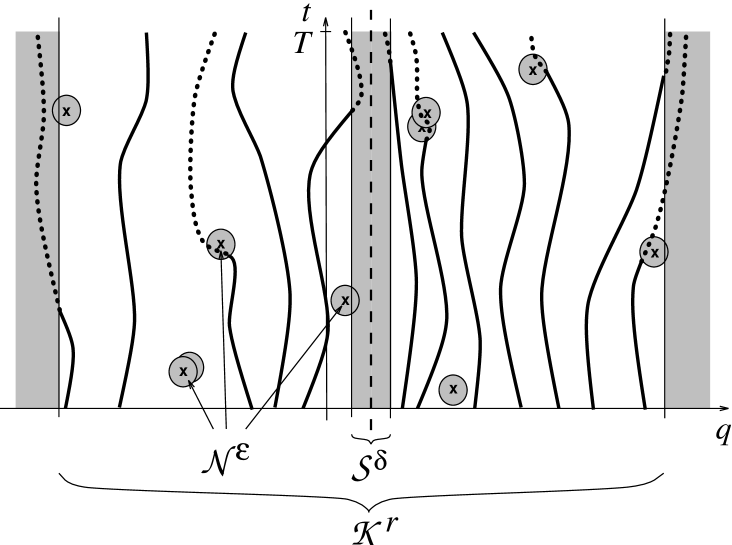
Figure 2: Bohmian trajectories run in the white area ${\cal G}^{\epsilon\delta r}=(({\cal K}^{r}\setminus{\cal S}^{\delta})\times{\rm I\!R})\setminus{\cal N}^{\epsilon}$. The set of singularities of the potential ${\cal S}\times{\rm I\!R}$ is dashed, nodes of the wave function are marked by x. Trajectories having crossed $\partial{\cal G}^{\epsilon\delta r}$ are dotted. By letting the grey neighborhoods ${\cal N}^{\epsilon}$ and ${\cal S}^{\delta}$ around the singularities of the velocity field shrink and the sphere ${\cal K}^{r}$ blow up, the set of dotted trajectories shrinks to a set of measure zero.

Consider now neighborhoods around the singularities of the velocity field: ${\cal N}^{\epsilon}$, a (configuration-space-time) neighborhood of thickness $\epsilon$ around the set of nodes ${\cal N}$ of the wave function, ${\cal S}^{\delta}$, a (configuration space) neighborhood of thickness $\delta$ around the set of singularities of the potential ${\cal S}=\partial\Omega$, and ${\cal K}^{r}$, a sphere in configuration space of radius $r$ to control escape to infinity. ${\cal G}^{\epsilon\delta r}$ denotes the set of “$\epsilon$-$\delta$-$r$-good” points in configuration-space-time: ${\cal G}^{\epsilon\delta r}=(({\cal K}^{r}\setminus{\cal S}^{\delta})\times{\rm I\!R})\setminus{\cal N}^{\epsilon}$ (see Figure 2).

A Bohmian trajectory approaching a singularity of the velocity field or infinity first has to cross the boundary of ${\cal G}^{\epsilon\delta r}$. From (9), we obtain the following bound for the probability of a “bad event” in the time interval $[0,T]$: for all $0<T,\epsilon,\delta,r<\infty$

$$P^{\psi_{0}}(\tau^{+}<T) \leq P^{\psi_{0}}({\cal G}_{0}\setminus{\cal G}^{\epsilon\delta r}_{0})\ +\ \int_{\partial{\cal G}^{\epsilon\delta r}\cap({\rm I\!R}^{3N}\times[0,T])}|J^{\psi_{t}}(q)\cdot n(q,t)|\,d\sigma$$ (10)

$$\leq P^{\psi_{0}}({\cal G}_{0}\setminus{\cal G}^{\epsilon\delta r}_{0})\ +\ {\bf N}(\epsilon,\delta,r)\ +\ {\bf S}(\delta)\ +\ {\bf I}(r)$$

with

$$\begin{array}[]{l}\displaystyle{\bf N}(\epsilon,\delta,r)\ =\ \int_{\partial{\cal N}^{\epsilon}\cap(({\cal K}^{r}\setminus{\cal S}^{\delta})\times[0,T])}|J^{\psi_{t}}(q)\cdot n(q,t)|\,d\sigma,\\ \displaystyle{\bf S}(\delta)\ =\ \int_{(\partial{\cal S}^{\delta}\cap\Omega)\times[0,T]}|J^{\psi_{t}}(q)\cdot n(q,t)|\,d\sigma,\\ \displaystyle{\bf I}(r)\ =\ \int_{(\partial{\cal K}^{r}\cap\Omega)\times[0,T]}|J^{\psi_{t}}(q)\cdot n(q,t)|\,d\sigma.\end{array}$$

By proving that for appropriate choices of sequences $\epsilon\to 0$, $\delta\to 0$, and $r\to\infty$ the right hand side of (10) gets arbitrarily small we show that for all $T>0$, $P^{\psi_{0}}(\tau^{+}<T)=0$, and thus $P^{\psi_{0}}(\tau^{+}<\infty)=0$. From time reversal invariance we obtain that also $P^{\psi_{0}}(\tau^{-}>-\infty)=0$, and that altogether the solutions of Bohm’s equation (2) with the velocity field (3) are global for almost all initial configurations.

Heuristically, it is rather immediate that the flux integrals ${\bf N}$, ${\bf S}$, and ${\bf I}$ get arbitrarily small as $\epsilon\to 0$, $\delta\to 0$, and $r\to\infty$. For ${\bf N}$, observe that the flux $J^{\psi}=0$ at the nodes of the wave function. From the continuity of $\psi$, $J^{\psi}$ is small in the vicinity of ${\cal N}$. Furthermore, the nodal set ${\cal N}$ itself is generically small: since $\psi$ is a complex function, the set where $\psi_{t}(q)=0$, i.e. ${\rm Re}\,\psi_{t}(q)=0$ and ${\rm Im}\,\psi_{t}(q)=0$, is generically of codimension 2 in configuration-space-time. Thus the area of $\partial{\cal N}^{\epsilon}$ should be small. Of the set $\cal S$ of singularities of the potential $V$, we assume in Berndl, Dürr, Goldstein, Peruzzi, Zanghì 1995 that it be contained in a union of a finite number of $(3N-3)$-dimensional hyperplanes, as is certainly the case for the $N$-particle Coulomb interaction $V=V_{\rm Coulomb}$ and the $N$-electron atom $V=V_{\rm atom}$. The area of $\partial{\cal S}^{\delta}$ is therefore very small. Moreover, in certain cases it is required as a boundary condition for self-adjointness of the Hamiltonian that the flux into the singularities of $V$ vanishes, see below. That the flux to infinity is small can be derived from the fact that the quantum flux $J^{\psi_{t}}(q)$ tends rapidly to 0 as $|q|\to\infty$, which follows from the square integrability of $\psi$ and $\nabla\psi$, i.e. from the normalizability of the $|\psi|^{2}$-distribution and finite “kinetic energy.” These conditions are automatically fulfilled for the considered class of potentials for $\psi_{0}\in C^{\infty}(H)$, which is just what we required for the existence of a global classical solution of Schrödinger’s equation.

We are thus lead back to the question of the existence of global classical solutions of Schrödinger’s equation! In fact, the connection between the global existence of Bohmian trajectories and global solutions of Schrödinger’s equation is most remarkable. The clue is the quantum flux $J^{\psi}$, which in Bohmian mechanics has the interpretation of a flux of particles moving along deterministic trajectories with velocity $v^{\psi}$: The condition that there is no flux into the critical points ensures firstly, as explained above, that the Bohmian configuration will not reach the critical points and thus exists globally. Secondly, it provides suitable boundary conditions for the domain of the Hamiltonian ${\cal D}(H)$ such that the Hamiltonian will be self-adjoint on ${\cal D}(H)$ and thus Schrödinger’s equation has global unique solutions as explained in Section 2. This connection is realized by considering that from integration by parts

$$\int_{M}\psi^{\ast}(H\psi)\,dq-\int_{M}(H\psi^{\ast})\psi\,dq\;=\;-i\hbar\int_{\partial M}j^{\psi}\cdot n\,ds,$$

for $M={\cal K}^{r}\backslash{\cal S}^{\delta}$, and thus by the self-adjointness of the Hamiltonian

$$\lim_{\delta\rightarrow 0,r\rightarrow\infty}\left(\int_{\partial{\cal S}^{\delta}\cap{\cal K}^{r}}j^{\psi}\cdot n\,ds\,\,+\,\,\int_{\partial{\cal K}^{r}\setminus{\cal S}^{\delta}}j^{\psi}\cdot n\,ds\right)\ =\ 0.$$

This is only slightly weaker than the vanishing of ${\bf S}(\delta)$ and ${\bf I}(r)$ in the limit $\delta\to 0$, $r\to\infty$, which is part of our sufficient condition for global existence of Bohmian trajectories. Moreover, in situations where the self-adjoint extension of $\widetilde{H}$ (cf. Section 2) is not unique, the particle picture of Bohmian mechanics supplies an interpretation of the different possible boundary conditions yielding different time evolutions of the wave function and thus a basis for the choice of one over the others. (For more on these points, see Berndl, Dürr, Goldstein, Peruzzi, Zanghì 1995.)

In this way, the point of view of Bohmian mechanics provides genuine understanding to the mathematics around the self-adjointness of Schrödinger Hamiltonians! Usually, the self-adjointness of the Hamiltonian—via its equivalence to the existence of a unitary group—is motivated by the conservation of $|\psi|^{2}$-probability. Probability of what? The standard answer—the probability of finding a particle in a certain region—is justified by Bohmian mechanics: A particle is found in a certain region because, in fact, it’s there. By incorporating the positions of the particles into the theory, and thus by interpreting $|\psi|^{2}$ as a probability density of particles being and the quantum flux $J^{\psi}$ as a flux of particles moving, Bohmian mechanics can be regarded as providing the foundation for all intuitive reasoning in quantum mechanics.

Figure 1: Sketch of the course of Bohmian trajectories for the wave function (4). Nodes of the wave function are marked by dots.

Footnotes

1     If only the expectation of $H^{2}$, the squared energy, is finite, $\psi_{0}\in{\cal D}(H)$, “Schrödinger’s equation holds in the $L^{2}$-sense,” i.e. $\displaystyle i\lim_{h\to 0}\frac{\psi_{t+h}-\psi_{t}}{h}=H\psi_{t}$, where the equality and convergence of the limit holds with respect to the Hilbert space norm and not pointwise as expressed by Schrödinger’s equation.

2     In this (one-dimensional) example the system explodes only after infinitely many two particle collisions; thus it does not describe a genuine pseudocollision.

References

Arnol’d, V.I. (1963), “Small denominators and problems of stability of motion in classical and celestial mechanics,” Russian Mathematical Surveys 18(6), 85–191. (Also: Arnol’d, V.I. (1989) Mathematical methods in classical mechanics. New York, Springer.)

Berndl, K., Dürr, D., Goldstein, S., Peruzzi, G., Zanghì, N. (1995), “On the global existence of Bohmian mechanics,” to appear in Communications in Mathematical Physics

Bohm, D. (1952), “A suggested interpretation of the quantum theory in terms of “hidden” variables I, II,” Physical Review 85, 166–179, 180–193.

Diacu, F.N. (1992), Singularities of the N-body problem. Montréal, Les Publications CRM. (Also: Diacu, F.N. (1993), “Painlevé’s Conjecture,” Mathematical Intelligencer 15, 6–12.)

Dürr, D., Goldstein, S., Zanghì, N. (1992a), “Quantum equilibrium and the origin of absolute uncertainty,” Journal of Statistical Physics 67, 843–907.

Dürr, D., Goldstein, S., Zanghì, N. (1992b), “Quantum mechanics, randomness, and deterministic reality,” Physics Letters A 172, 6–12.

Gerver, J.L. (1991), “The existence of pseudocollisions in the plane,” Journal of Differential Equations 89, 1–68.

Kato, T. (1951), “Fundamental properties of Hamiltonian operators of Schrödinger type,” Transactions of the American Mathematical Society 70, 195–211.

Mather, J., McGehee, R. (1975), “Solutions of the collinear four body problem which become unbounded in finite time” in J. Moser (ed.), Dynamical Systems: Theory and Applications. Berlin, Springer.

Moser, J. (1973), Stable and Random Motions in Dynamical Systems. Princeton, Princeton University Press.

Reed, M., Simon, B. (1975), Methods of Modern Mathematical Physics II. San Diego, Academic Press. (Also: Simon, B. (1977), “An introduction to the self-adjointness and spectral analysis of Schrödinger operators” in W. Thirring, P. Urban (eds.), The Schrödinger Equation. Wien, Springer, pp. 19–42.)

Xia, Z. (1992), “The existence of noncollision singularities in Newtonian systems,” Annals of Mathematics 135, 411–468.