Abstract

Recent results suggest that quantum mechanical phenomena may be interpreted as a failure of standard probability theory and may be described by a Bayesian complex probability theory.

There is more to probability theory than proving theorems in a particular mathematical system. One is also in a position to make predictions about real physical systems by adding extra assumptions to the standard axioms. Such predictions are necessarily subject to experimental test, and, to the extent that one believes in the extra assumptions, such tests may be interpreted as testing the correctness of probability theory itself. Now this may already seem like an odd point of view, especially here, since this conference series itself provides a most impressive record of success for probability theory in a vast array of situations with no indication of a problem – so why is there any reason to doubt probability theory? Here I think that there is a historical effect: probability theory may actually be failing all the time, it’s just that the situations where a failure occurs are called “quantum mechanical phenomena” and thus appear in physics conferences instead of in probability theory conferences. This suggests that perhaps there is something wrong with probability theory after all, and that this may be where quantum mechanical effects come from. Let’s adopt this point of view and see where it leads [Youssef (1991), Youssef (1994), Youssef (1995)].

An obvious place to test our new point of view is the two–slit experiment where, as everyone knows, the fact that an interference pattern is observed even if one particle is sent through at a time, forces us to conclude that it is not true that a particular particle either goes through slit $\#1$ or through slit $\#2$; in general, then, a particle cannot be said to follow a path through space. This is the “wave–particle duality,” the basic effect in quantum mechanics. Notice, however, that from our new point of view, the standard argument has a hole in it due to it’s essential reliance on probability theory. For a position $x$ on the screen where there is a dip in the interference pattern, one reaches a contradiction by noticing that

$${\rm P}(x)={\rm P}(x\ via\ slit\#1)+{\rm P}(x\ via\ slit\#2)\geq{\rm P}(x\ via\ slit\#1)$$

means that opening the second slit should not cause the probability to arrive at $x$ to decrease. But if we are willing to modify probability theory, then the standard argument and it’s surprising conclusions do not necessarily follow. In fact it is clear that in order to escape the standard conclusions, a modified probability theory must provide a way for probabilities to cancel each other and so an obvious first guess is to allow probabilities to be complex numbers. Here, of course, the argument grinds to a halt for a frequentist since frequencies are not the complex numbers. However, as Bayesians, we are not completely out of options because for us, probabilities start out only as (real and non–negative) measurements of “likelihood” where the frequency meaning for this likelihood is derived after the fact. Similarly, we might consider a complex “likelihood” and see if a frequency meaning can be found for this as well. In fact, the simplest thing to do is to take Cox’s assumptions[Cox (1946)] and just drop the restriction that probabilities be real and non–negative. In this case, it turns out that Cox’s entire argument follows as before and one ends up with “complex probability theory” having the same form as the probability theory that you’re used to except that probabilities are complex. For any propositions $a$, $b$ and $c$,

$$(a\rightarrow b\wedge c)=(a\rightarrow b)(a\wedge b\rightarrow c)$$

$$(a\rightarrow b)+(a\rightarrow\neg b)=1$$

$$(a\rightarrow false)=0$$

where I have written the complex probability that proposition $b$ is true given that proposition $a$ is known as “$(a\rightarrow b)$” (to be read: “$a$ goes to $b$”) reserving the more familiar notation $P(b|a)$ for standard $[0,1]$ probabilities.

Given our complex probability theory we would like to continue in parallel with the Bayesian development and construct a frequency meaning for complex probabilities. Recall that for standard probability, this works by supposing that the probability of something is $p$ and considering $N$ copies of that situation with $f=n/N$ successes. Using the central limit theorem $f$ is asymptotically gaussian with mean $p$. Then, since the probability for $f$ to be in any interval not containing $p$ can be made arbitrarily small by increasing $N$, this fixes the frequency meaning for $p$. Essentially, the frequency meaning of $p$ rests on the extra assumption that an arbitrarily small probability for $f$ to be in some interval means that $f$ in fact will never be observed to be in that interval in a real experiment. The situation is not quite so simple in complex probability theory because a zero complex probability does not in general mean that the corresponding event will never happen. However, we can proceed by assuming that this extra condition is true for a special set of propositions $U$ called the “state space.” Let’s also assume that this $U$ satisfies the following for $x,y\in U$, propositions $a,b$, time $t\leq t^{\prime}\leq t^{\prime\prime}$:

$$x_{t}\wedge y_{t}=false\ {\rm if}\ x\neq y$$

$$(a_{t}\rightarrow b_{t^{\prime\prime}})=(a_{t}\rightarrow U_{t^{\prime}}\wedge b_{t^{\prime\prime}})$$

$$(a_{t}\wedge x_{t^{\prime}}\rightarrow b_{t^{\prime\prime}})=(x_{t^{\prime}}\rightarrow b_{t^{\prime\prime}})$$

where subscripts denote time, as in “$a_{t}$” meaning “$a$ is true at time $t$,” and where a set of propositions with a subscript denotes the $or$ of each element with the same subscript, as in $U_{t}=\vee_{x\in U}x_{t}$. These are just Markovian style axioms intuitively corresponding to “the system has a state.” Roughly, the system cannot be in two different states at the same time (II.a), the system is in some state at each intermediate time (II.b) and the knowledge that a system is at some point in the state space makes all previous knowledge irrelevant (II.c). We assume that $U$ is a measure space with $(a_{t}\rightarrow U_{t^{\prime}})=\int_{x\in U}(a_{t}\rightarrow x_{t^{\prime}})$. Note the clash of terminology where the Hilbert space of standard quantum mechanics is sometimes also called the “state space.” Here $U$ is only a measure space of propositions.

Given I and II, one can repeat the standard argument for the expression

$$Prob(a_{t},b_{t^{\prime}})={{\int_{x\in U}|a_{t}\rightarrow b_{t^{\prime}}\wedge x_{t^{\prime}}|^{2}}\over{\int_{x\in U}|a_{t}\rightarrow x_{t^{\prime}}|^{2}}}$$

which predicts the frequency that $b$ is found to be true at time $t^{\prime}$ given that $a$ is known at a previous time $t$. Although Prob as defined is able to predict the frequencies for outcomes of any experiment, it fails to extend to propositions involving mixed times (e.g. $b_{t^{\prime}}\wedge c_{t^{\prime\prime}}$, $t^{\prime\prime}>t^{\prime}$). This is an interesting point because it is exactly this failure that allows complex probability theory to escape Bell’s theorem[Youssef (1995)]. Also, although I don’t have a sharp result, it is seems likely that this effect disappears in a classical limit, thus explaining why standard probability theory works in the classical domain.

Immediate consequences of axioms I.a–I.c and II.a–II.c include facts familiar from probability theory such as $(a\rightarrow true)=1$, $(a\rightarrow b\vee c)=(a\rightarrow b)+(a\rightarrow c)-(a\rightarrow b\wedge c)$, and if $(a\rightarrow b)\neq 0$, then $(a\wedge b\rightarrow c)=(a\rightarrow c)(a\wedge c\rightarrow b)/(a\rightarrow b)$ (Bayes Theorem). Following standard probability theory, propositions $a$ and $b$ are said to be independent if $(q\wedge a\rightarrow b)=(q\rightarrow b)$ for all $q$ and, just as in standard probability theory, “locality” enters via assumptions of independence. For instance, if experiments $e_{1}$ and $e_{2}$ have possible results $r_{1}$ and $r_{2}$ respectively, then the assumptions that $\{r_{1},r_{2}\}$, $\{e_{1},r_{2}\}$, and $\{e_{2},r_{1}\}$ are independent imply

$$(e_{1}\wedge e_{2}\rightarrow r_{1}\wedge r_{2})=(e_{1}\rightarrow r_{1})(e_{2}\rightarrow r_{2})$$

as one would expect from, for example, two experiments which have nothing to do with each other. Other simple consequences of the axioms are described in references 1-4 including

• The Path Integral

• The Superposition Principle

• The Expansion Postulate

• The Schrödinger/Klein–Gordon Equations for $U=R^{d}$

where the standard wavefunction $\Psi(x,t)$ is proportional to the complex probability

$$(Everything\ that\ you\ know\ about\ the\ system\rightarrow x_{t})$$

making the Bayesian status of the wavefunction obvious. In particular, the same system may be described by different wavefunctions depending upon what is known and such wavefunctions can clearly not be “the state of the system” in any reasonable sense.

To get a feeling for how things work, let’s consider a typical interferometer as shown in figure 1.

Figure 1.  : A simple interferometer where a particle enters as indicated and encounters a beam splitter ($S_{1}$), a mirror ($M_{1}$ or $M_{2}$), a second beam splitter ($S_{2}$) ending up either in detector $D_{1}$ or in detector $D_{2}$.

Particles enter the device one at a time, pass through a beam splitter, hit one of two mirrors and pass through a second beam splitter ending up either in detector $D_{1}$ or in $D_{2}$. Although it looks perfectly possible for a particle to end up in $D_{2}$, experimentally we mysteriously find that this never happens. All the particles register in $D_{1}$. In standard quantum theory, one describes this situation by saying that there are two paths for a particle to go from the source to $D_{2}$. The amplitude for these paths have opposite signs and since the probability is the square of the total amplitude, this explains why particles never enter $D_{2}$. Now let’s consider a modified situation (figure 2) where a device is attached to one of the mirrors which is able to detect if the mirror was struck by the particle.

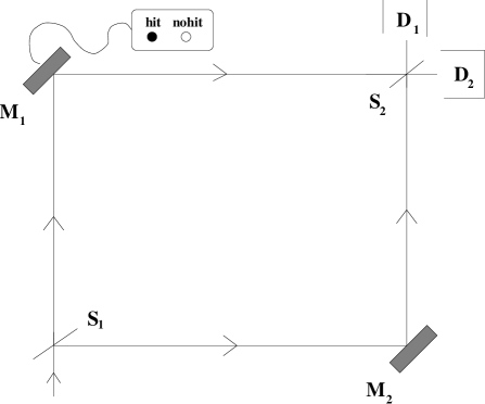
Figure 2.  : A interferometer similar to the one shown in figure 1. The device is attached to the mirror $M_{1}$ records whether $M_{1}$ was struck by the particle or not.

After each particle passes through, the device either indicates “hit” or “no hit.” Experimentally, we find that the results are now different with about half of the particles ending up in detector $D_{2}$. How can we explain this? In standard quantum mechanics there are still two paths for a particle to reach $D_{2}$ as before. However, since we can now tell which path was taken by the particle by inspecting the hit/no–hit device, the amplitudes for the two paths no longer interfere. This is a special case of the general principle:

• Paths interfere only if there is no way of knowing which path was taken, even in principle.

This is a rather mysterious statement since it suggests that whether or not you can deduce which path was taken somehow affects the behavior of the particle. Also, it is not clear what “even in principle” means here or what happens if, for example, the hit/no–hit device works with, say, 99% efficiency. Even so, the basic prediction of this principle is correct and this raises the question of whether there is an analogous principle in complex probability theory and whether the predictions are the same. You can indeed easily deduce from the axioms and the definition of $Prob$ that

• Paths interfere if and only if they end at the same point in U.

and this appears to give the same predictions as the more mysterious sounding standard quantum mechanical principle. For instance, within complex probability theory, the situation of figure 1 could be described by a state space $R^{3}$ (assuming that the particle is spinless) in which case the complex probability to arrive at $D_{2}$ is the sum of the complex probabilities for two paths, which also cancel, just as in standard quantum mechanics. In the situation shown in figure 2, one simply notes that the state space $R^{3}$ is evidently no longer sufficient to describe the system. If one extends the state space to, say, $U=R^{3}\times\{hit,nohit\}$, then the interference is lost because the two paths for reaching $D_{2}$ now end at different points in $U$. There is also a continuum between this result, where the hit/no–hit device is assumed to work perfectly, and a situation where the device works so badly that the propositions “hit” and “no–hit” are independent of which path the particle is taking. In this case, you can easily show that the original effect is restored[Youssef (1994)].

Of course, standard quantum mechanics is perfectly capable of handling a situation like that of figure 2. It’s just that a rigorous treatment of the problem with a Hilbert space including the hit/no–hit device where the state vector evolves under the action of a Hamiltonian would be rather difficult, especially considering the simplicity of the answer. This helps to explain the popularity of “which path” style arguments in spite of their ambiguity. Here complex probability theory has the advantage that simple assumptions about a system can rigorously be encorporated without having to decide what the assumptions mean in terms, for example, of solutions to the Schrödinger equation. A rigorous treatment of these problems within quantum mechanics would also have to address the issue of whether the initial state is “mixed” or not since not all situations in quantum mechanics can be described by a vector in a Hilbert space, some require “statistical mixtures” of vectors in a Hilbert space. This provides an interesting test for complex probability theory. Since ordinary “statistical mixtures” are no longer available to us, situations requiring “mixed states” had better be handled within the existing axioms. These situations appear to indeed be handled quite smoothly and naturally within the complex probability theory described here[Youssef (1994)].

To take an example with more detailed predictions, consider a single scalar particle with $U=R^{d}$ and consider a sequence of propositions $x_{o},x_{1},\dots,x_{n}$ in $U=R^{d}$ where each $x_{j}$ implicitly has a time subscript $t_{j}$ with $t_{j+1}-t_{j}=\tau>0$. As always, $(x_{o}\rightarrow x_{n})$ is given by the “path integral”

$$(x_{o}\rightarrow x_{n})=\int_{x_{1}}\dots\int_{x_{n-1}}(x_{o}\rightarrow x_{1})(x_{1}\rightarrow x_{2})\dots(x_{n-1}\rightarrow x_{n}).$$

Of course, there is a path integral in standard quantum mechanics as well[(5)] where one proceeds to dynamics by assuming that the amplitude for a path is proportional to $e^{iA}$ where the “action” $A$ is the time integral of a classical Lagrangian for the system. Here we can avoid these extra assumptions by repeating the same argument within each $\tau$ sized interval making $n$ sub–path integrals (figure 3) with time step $\epsilon=\tau/N$.

Figure 3.  : For $x_{0},x_{n}\in U$, the complex probability $(x_{0}\rightarrow x_{n})$ is equal to a “path integral” over $x_{1},x_{2},\dots,x_{n-1}$ with time step $\tau$. The argument can be repeated making $n$ sub–path integrals with time step $\epsilon$.

By letting both $\tau$ and $\epsilon$ go to zero, one can extract a central–limit–theorem–like result where for small $|z|$ and small $\tau$, $(x_{t}\rightarrow(x+z)_{t+\tau})$ is given by

$${1\over(2\pi\tau)^{{d\over 2}}\sqrt{{\rm det}[\nu]}}{\rm exp}(-\tau[{1\over 2}({z_{j}\over\tau}-\nu_{j})W_{jk}({z_{k}\over\tau}-\nu_{k})+\nu_{0}])$$

where $\nu_{o}(x)$, $\nu_{j}(x)$, $\nu_{jk}(x)$ and $W_{jk}(x)$ are moments of $\mu(x,z,\tau)\equiv(x_{t}\rightarrow(x+z)_{t+\tau})$ defined by

$\nu_{0}(x)=\int_{z\in U}\mu_{\tau}(x,z,0)$

$\nu_{j}(x)=\int_{z\in U}\mu_{\tau}(x,z,0)z_{j}$

$\nu_{jk}(x)=\int_{z\in U}\mu_{\tau}(x,z,0)z_{j}z_{k}$

with $W_{jk}=M_{jl}M^{T}_{lk}\omega_{l}$ where $M$ is the matrix which diagonalizes $\nu_{jk}$ such that $M^{T}_{lj}\nu_{jk}M_{km}=\delta_{lm}/\omega_{l}$. With velocity $v_{j}$ given by the limit of $z_{j}/\tau$, the above propagator is equivalent to the Lagrangian

$${\cal L}(x,v)={i\over 2}(v_{j}-\nu_{j})W_{jk}(v_{k}-\nu_{k})-i\nu_{0}$$

where we recognize $\nu_{j}(x)$ and $\nu_{o}(x)$ as the electromagnetic fields and where $W_{jk}(x)$ contains the particle mass and space–time metric. Notice that we have not assumed Lorentz or gauge invariance to get this result. The claim is that this is the only Lagrangian consistent with the state space $R^{d}$.

Since our complex probability theory is both “realistic” in the sense of assuming that a particle does come through one slit or the other in the two slit experiment (II.b) and local in the sense of accepting locality assumptions as assumptions of “complex statistical independence,” you might think that we would run afoul of Bell’s theorem or other more recent limitations on local realistic theories. As I’ve already mentioned, Bell’s result does not follow in complex probability theory. This means that although Bell’s result has almost universally been interpreted as ruling out local realistic theories, from our more general point of view, it forces a choice between local realism and standard probability theory. In fact, Bell’s result can be interpreted as another little hint that there is something wrong with probability theory. Besides Bell, there are a large number of more recent limitations on local realistic theories, each of which provides a test of the complex probability formulation. Details are available only for three representative results of this type (including Bell) where complex probability theory appears not to be excluded[Youssef (1995)].

You might expect that if quantum mechanical phenomena can be described by complex probability theory, the Bayesian view might help in understanding some of the long standing semi–paradoxical measurement and observer questions in quantum mechanics. Here, it’s helpful to first think about a purely classical experiment where a single coin is flipped and then uncovered, revealing that it landed “heads.” From the Bayesian point of view, of course, the situation before the observation could be described by the distribution $(1/2,1/2)$ and after observing heads our description would be adjusted to $(1,0)$. The problem is, what would you say to a student who then asks:

• Yes, but what causes $(1/2,1/2)$ to evolve into $(1,0)$? How does it happen?

Here we recognize a victim of a severe form of “Mind Projection Fallacy”[Jaynes (1989)] where the person asking this question has confused what they know about the system with the system itself. With the Bayesian view of complex probabilities, it is clear that this same mistake is possible in quantum mechanics as well, where one would now be mistaking a wavefunction for the state of the system. This very view, however, is the standard picture of quantum mechanics and so it is hardly surprising that similar mysteries arise. This view is also implicit in questions such as

• Can the wavefunction be measured?

• What is the source of the non–local effects in EPR?

• Can macroscopic superpositions be created?

• Is the Universe in a pure state?

Although these are active research questions, it seems inescapable to me that if quantum phenomena are correctly described by a Bayesian probability theory, then all of these questions have trivial answers and they all ultimately fall into the same category as the student’s question about coin flipping experiments.

For this audience, I hardly need to point out that the ideas that we have discussed here may not only clarify the meaning of quantum mechanics, but may also lead to ways of improving quantum mechanical calculations using prior knowledge in the same sense that prior knowledge is used to improve probability calculations in Bayesian Inference.

References

- Youssef (1991) S.Youssef, Mod.Phys.Lett. A6, 225 (1991).
- Youssef (1994) S.Youssef, Mod.Phys.Lett. A9, 2571 (1994).
- Youssef (1995) S.Youssef, Phys.Lett. A204, 181(1995).
- Cox (1946) R.T.Cox, Am.J.Phys. 14, 1(1946).
- (5) R.P.Feynman and H.R.Hibbs, Quantum Mechanics and Path Integrals (McGraw–Hill, 1965).
- Jaynes (1989) E.T.Jaynes, in Maximum Entropy and Bayesian Methods, ed. J.Skilling(Kluwer, 1989).