Newtonian Quantum Gravity

Abstract

We develop a nonlinear quantum theory of Newtonian gravity consistent with an objective interpretation of the wavefunction. Inspired by the ideas of Schrödinger, and Bell, we seek a dimensional reduction procedure to map complex wavefunctions in configuration space onto a family of observable fields in space–time. Consideration of quasi–classical conservation laws selects the reduced one–body quantities as the basis for an explicit quasi–classical coarse–graining. These we interpret as describing the objective reality of the laboratory. Thereafter, we examine what may stand in the role of the usual Copenhagen observer to localize this quantity against macroscopic dispersion. Only a tiny change is needed, via a generically attractive self–potential. A nonlinear treatment of gravitational self–energy is thus advanced. This term sets a scale for all wavepackets. The Newtonian cosmology is thus closed, without need of an external observer. Finally, the concept of quantization is re–interpreted as a nonlinear eigenvalue problem. To illustrate, we exhibit an elementary family of gravitationally self–bound solitary waves. Contrasting this theory with its canonically quantized analogue, we find that the given interpretation is empirically distinguishable, in principle. This result encourages deeper study of nonlinear field theories as a testable alternative to canonically quantized gravity.

I Introduction

The Schrödinger interpretation of the wavefunction (Schrödinger 1928, Barut 1988) would be extremely useful if it were consistent. Then quantum theory would provide a direct means to address the problem of particle structure, and an immediate route to construct generally covariant field theories founded upon analogy with classical continuum physics.

Of course, there are two long–standing problems that obstruct consideration of this historical proposal. Firstly, quantum interactions entangle states, leading to non–separable densities in configuration space. Secondly, dispersion is ever present, so that general localized solutions are unavailable (Schrödinger 1926). Taken together, these difficulties are insurmountable in a linear theory, and the continuum option must fail.

In this paper we show that both difficulties can be overcome within a larger theory based upon nonlinear wave–equations. For this purpose we combine: the mathematics of Kibble (1978,1979), and Weinberg (1989); the continuum viewpoint of Schrödinger (1928); the measurement scenario of Penrose (1993); and the physical mechanism of environmentally induced decoherence (Zurek 1981,1982,1991).

The argument hinges upon exploiting the verified classical conservation laws to select an explicit quasi–classical coarse–graining (cf. Gell-Mann and Hartle 1993). This approach is closest in spirit to Bell’s idea of beables; some special class of quantities representing the reality on which laboratory observations are founded (Bell 1973). Here reduced one–body densities and currents are advanced to play this role.

Nonlinearity is then invoked to obtain a generic physical mechanism to suppress the macroscopic dispersion which would otherwise spread out the observable fields. Thus nonlinearity is to assume that role now given to observers. Assuming that an objective theory should be free of an external observer at all levels, we are led to constrain the nonlinearity by demanding this at the simplest level.

Since gravitation is universally attractive, and is not directly tested at the quantum level, we focus upon it as the means to suppress dispersion. The outcome is a possible new avenue to a theory of individual events — although, for simplicity, this paper treats only Newtonian gravity to secure the foundation for more general nonlinear theories.

The key motivation behind this line of enquiry is the cosmological conundrum posed by quantum measurement (Bell 1981). Nonlinear theories offer new modes of physical interaction that do not quantum entangle. Since the observer is now treated as a separable (i.e. non–entangled) participant in quantum mechanics, nonlinear wave–equations are an attractive option for the physical treatment of measurements (Jones 1994b). However, their interpretation remains problematic. This suggests that we look for a specific theory, using self–consistency and the question of measurement as guides (Jones 1995).

For one massive scalar particle with nonlinear gravitational self–interactions the goal of observer–free localization is achieved, and the theory is self–consistent. Correspondence principle arguments are then used to obtain a many–particle theory. The gravitational wave–equation lies within the generalized dynamics of Weinberg (1989), and resembles the approximate equations of Hartree–Fock electromagnetism (Brown 1972).

Quasi–classical coarse–graining plays a central role in the physical interpretation of these equations according to the continuum viewpoint of Schrödinger (1928). As soon as the initial obstructions to it are overcome one realizes that quantum field theory is perhaps open to a significant reformulation in toto.

For instance, as Barut (1990) has noted in his attempt to reformulate QED as a linear theory with nonlinear self–energy terms, the time–like component of a particle current need not be of definite sign if it is a charge density, and not a probability density. Hence the Dirac equation might be viewed as describing a single entity. Then one might simplify the conceptual basis of quantum field theories, to free them from the shackles of perturbative method, and render them closed theories applicable to the entire cosmos. Thus one may perceive already the outlines for a program of unification based upon nonlinearity, the Schrödinger interpretation, and a more physical approach to quantum measurement.

Since the interpretation of nonlinear theories has been a major historical stumbling block the early material, sections $2$ through $6$, is devoted to addressing this within a continuum philosophy a lá Schrödinger (1928). Coarse–graining is dealt with early on, in section $3$. Then, in section $7$, we generalize Lagrangian dynamics to complex fields in configuration space. In sections $8$ through $12$, we construct the nonlinear theory of pure Newtonian gravity. Its relevance is then discussed in the concluding section.

II Continuum physics and nonlinearity

Schrödinger (1928), Einstein (1956), and de Broglie (1960), were each dissatisfied with the Copenhagen interpretation, and sought some means to rid quantum mechanics of its reliance upon the philosophical notion of observers. One possible option they considered is to introduce nonlinearity, so that the microscopically tested superpositions are inhibited at the macroscopic level of the observing instrument. The difficulty is to locate a candidate nonlinearity, and to interpret such theories consistently. Here we reconsider the continuum viewpoint espoused by Schrödinger (1928), and seek to complete his conception.

The easiest way to appreciate the historical ambiguity surrounding the interpretation of the wavefunction is to examine a nonlinear wave–equation, such as

$$i\hbar\frac{\partial\psi({\bf x},t)}{\partial t}=\left\{-\frac{\hbar^{2}}{2m}\nabla^{2}\pm\kappa|\psi({\bf x},t)|^{2}\right\}\psi({\bf x},t),$$ (1)

(later we consider a general self–potential $V[\psi,\psi^{*}]$ in place of the term $\pm\kappa|\psi({\bf x},t)|^{2}$). Such equations arise frequently as the Hartree–Fock approximation to an interacting quantum field theory (see e.g., Brown 1972, Kerman and Koonin 1976). Although of practical utility, they are generally ignored in discussions of fundamental physics - - — primarily because the program of canonical quantization leads always to a linear theory (Dirac 1958).

Most importantly, the orthodox Copenhagen interpretation demands linear equations. A measurement might occur at any instant, due to the intervention of an observer. In virtue of the split, between dynamics and the observational process, one must ensure that quantum evolution preserves transition probabilities. Wigner’s theorem asserts that the only continuous probability preserving maps on the space of states are linear unitary (for a recent review see Jordan (1991)). Linearity for unobserved systems is thus reconciled with — and demanded by — the postulate of a quantum jump during measurements.

To go beyond this simplistic idealized picture we need to recognize the pragmatism which lies at its root. It is a successful algorithm for conducting computations, but it ignores the physical basis of measurements. To probe coherent few–particle dynamics one must first ensure conditions of isolation. This we describe by introducing a single wavefunction for the object system — neglecting the rest of the Universe. However, subsequently this isolation must be broken — when a measurement is made. At this stage the theorem of Wigner becomes suspended, and the collapse postulate is invoked. In practice, one is then ascending the scale from the few particles of interest to the collective behaviour of many within the measuring apparatus. Therefore, it is natural to associate any breakdown of the superposition principle with emergent many–body nonlinearities.

Consider the quantum description of a many–body laboratory instrument, see Fig. 1. Through the collective evolution of its constituents it gives concrete form to information gained about the microscopic world. Although Copenhagen physics assumes a discrete picture of the microworld, the quasi–classical level resembles a continuum. Since our sole experience of the micro–world is founded in observations at this level (Bohr 1928,1949) one must admit the logical possibility of a continuum foundation to all physics. Given the huge gulf in scale ($\sim 10^{23}$ in number) between micro and macro physics, a continuum whole may well fluctuate (when stong fields are involved) to appear composed of discrete parts — the idealized point–like particles of Copenhagen quantum physics.

Bell (1973) has sought a more objective theory through his concept of “beables”, some class of quantities representing the objective status of observing instruments. Such beables are readily imagined as fields defined in ordinary space–time which describe the totality of the atomic world, and the observing instrument. The main conceptual problem is to recover the notion of elementary particles, as separate well–localized entities. The continuum field must appear composed of fluctuating indivisible parts, and we must ensure that any fundamental level of determinism is inaccessible to direct empirical control.

Here we treat particles as an idealized concept appropriate to the weak–field limit when observable continuum fields decompose into several distinct lumps. Then we may subsume Copenhagen physics as an ideal case, and employ it as a known limit to guide the formulation of new equations.

Some immediate guidance to a viable coarse–grained continuum interpretation may be found in practical many–body equations like (1). There the quantity $|\psi|^{2}$ is interpreted as denoting the density of particles in an aggregate. Examining (1), we construct the current

$${\bf j}({\bf x},t)=\frac{\hbar}{2mi}\left\{\psi^{*}({\bf x},t)\nabla\psi({\bf x},t)---\psi({\bf x},t)\nabla\psi^{*}({\bf x},t)\right\}$$ (2)

and so readily verify the equation of continuity

$$\frac{\partial\rho}{\partial t}+\nabla\cdot{\bf j}({\bf x},t)=0,$$ (3)

where $\rho({\bf x},t)=|\psi({\bf x},t)|^{2}$ (provided the nonlinear self–potential $V$ is real–valued).

Thus we can interpret macroscopic conserved currents in two different ways. They could describe the evolution, in probability density, of very many point–like particles spread as $\rho({\bf x},t)$, or the flow of continuum matter. Recall, both Born and Schrödinger, each employed current conservation to defend their respective interpretations. With the ancient Greeks, we may ask again: Does nature give preference to the discrete or continuum viewpoint?.

III Explicit quasi–classical coarse graining

So what are the problems with the continuum viewpoint? Firstly, the candidate for a macroscopic “beable” continuum field must be generated from a wave in configuration space. Secondly, we must explain how a physics based upon this assumption could exhibit the discrete and stochastic behaviour we observe in quantum experiments.

Evidently, the key avenue into such a theory must lie within that role now played by the Copenhagen observer. As soon as we drop the Born interpretation something must be found in place of the observer. Presently, this agent serves to connect wavefunctions with the laboratory reality. Therefore, the continuum coarse–graining must effect a similar mapping from the abstract mathematics into the concrete world of observations.

Since wavefunctions are generally formulated as fields on a configurational space–time, the mapping into observable fields must reduce fields in $N(3+1)$ dimensions down to the familiar $3+1$ dimensions apparent in the laboratory. Hence we conceive of an observable level whose dynamics is determined at an unobservable level, with the two levels linked by dimensional reduction. The idea is perhaps familiar already from string theory, where embarassing dimensions are compactified away, and one has the sophistication to recognize that mere mathematics is not reality, but can serve our efforts to model it.

Many such prescriptions are possible, so we must adopt some principle to guide the search. The avenue we take is to look for quasi–classical conservation laws, and confine attention to mappings which recover these. The rationale is clear: observable fields must display the observed conservation laws.

Consider, therefore, the many–body Schrödinger equation for $N$ particles, each of mass $m_{j}$. In accordance with established physics we describe these by a wavefunction $\Psi({\bf X};t)$, where ${\bf X}=({\bf x}_{1},\ldots,{\bf x}_{N};t)$ is a $3N$–vector in configuration space. The corresponding Schrödinger equation reads

$$i\hbar\frac{\partial\Psi({\bf X};t)}{\partial t}=-\sum_{j=1}^{N}\frac{\hbar^{2}}{2m_{j}}\nabla^{2}_{{\bf x}_{j}}\Psi({\bf X};t)+V[\Psi,\Psi^{*}]\Psi({\bf X};t),$$ (4)

where $V[\psi,\psi^{*}]$ is a general real–valued potential.

Higher dimensional conservation laws in configuration space are easily obtained from (4). For instance, one may form a $3N$–vector many–body current

$${\bf j}^{(N)}({\bf X};t)\equiv({\bf j}^{(1)}_{1}({\bf X};t),\ldots,{\bf j}^{(1)}_{N}({\bf X};t)),$$ (5)

composed of $N$ different $3$–vector partial currents

$${\bf j}^{(1)}_{j}({\bf X};t)\equiv\frac{\hbar}{2m_{j}i}\left\{\Psi^{*}({\bf X};t)\nabla_{{\bf x}_{j}}\Psi({\bf X};t)-\Psi({\bf X};t)\nabla_{{\bf x}_{j}}\Psi^{*}({\bf X};t)\right\},$$ (6)

along with the corresponding scalar density

$$\rho^{(N)}({\bf X};t)\equiv\Psi^{*}({\bf X};t)\Psi({\bf X};t).$$ (7)

Thus we obtain a many–body equation of continuity

$$\partial_{t}\rho^{(N)}({\bf X};t)+\partial_{\bf X}\bullet{\bf j}^{(N)}({\bf X};t)=0,$$ (8)

where “$\bullet$” denotes the natural $3N$–vector dot product.

Such conservation laws would normally be introduced to discuss the joint measurement of $N$ particles. To do this in practice would require $N$ detectors, each of them composed of many particles. Therefore, we put a particle picture aside, and concentrate upon how one is to describe the instrumental readout of a notional meter. The “needle” position is encoded jointly in the collective state of very many particles, and so a coarse–grained treatment will suffice, see again Fig. 1. In classical point mechanics the mass density

$$\rho({\bf x};t)=\sum_{j=1}^{N}m_{j}\delta({\bf x}-{\bf x}_{j}),$$ (9)

is one candidate to describe the substance of this pointer. In classical continuum physics we simply smear out each of the $N$ delta functions with a density $\rho_{j}(x_{j})$, and integrate over configuration space. In analogy with this familiar case the quantum entanglement may be submerged from direct view by integration of the many–body density (7).

Hence we obtain a reduced one–body density

$${\bf\rho}^{(1)}({\bf x};t)\equiv\int d^{3N}{\bf X}\,\sum_{j=1}^{N}\delta({\bf x}-{\bf x}_{j}){\bf\rho}^{(N)}({\bf X};t),$$ (10)

and the corresponding reduced one–body current

$${\bf j}^{(1)}({\bf x};t)\equiv\int d^{3N}{\bf X}\,\sum_{j=1}^{N}\delta({\bf x}-{\bf x}_{j}){\bf j}^{(N)}({\bf X};t).$$ (11)

In Copenhagen physics one would recognize these as describing the probability density and current for “finding” all $N$ particles at once, neglecting the correlations among them. This is exactly the kind of coarse–graining we require to describe quasi–classical instrumental readouts. Further, by integration of (8) we obtain

$$\partial_{t}\rho^{(1)}({\bf x};t)+\partial_{\bf x}\cdot{\bf j}^{(1)}({\bf x};t)=0,$$ (12)

a reduced one–body equation of continuity. Hence we recover the familiar quasi–classical law of (local) mass conservation, without appeal to an observer.

A suitable general prescription, consistent with these principles, is the familiar one–body field operator of standard many–body physics. Specifically, we consider the quantities

$$f({\bf x},t)\equiv\langle\Psi|\hat{F}({\bf x},t)|\Psi\rangle$$ (13)

where $|\Psi\rangle$ is the many–body state, and a typical one–body operator may be written

$$\hat{F}({\bf x},t)=\hat{\Psi}^{\dagger}({\bf x},t)F({\bf x},t)\hat{\Psi}({\bf x},t),$$ (14)

with $\hat{\Psi}^{\dagger}({\bf x},t)$, and $\hat{\Psi}({\bf x},t)$ the usual field creation and annihilation operators and $F({\bf x},t)$ is generally a $c$–number distribution (e.g. $-i\hbar\nabla$ for momentum). Thus we arrive at an explicit prescription for what Gell–Mann and Hartle (1993) have referred to as a quasi–classical coarse graining of the quantum micro–reality.

IV Hypothesis of restricted observables

To complete the interpretation we advance a simple hypothesis: Only reduced one–body quantities are directly observable — all other observations must be derived from these. The purpose behind this postulate is to secure the foundations for a continuum theory, in which there is no need to introduce an external observer that must “find” the many particles which comprise a macroscopic instrumental readout.

Now the correspondence principle of Bohr (1928) is met directly in the construction of the observable level along with the non–classical property of quantum entanglement. Via coarse–graining this property becomes reconciled with our direct experience of apparently continuous quantities formulated in a $3+1$ dimensional space–time. However, unlike classical continuum physics, the dynamics of the observable fields drawn above is not determined by their values, but rather those of $\Psi$.

Obviously, quantum non–separability remains important in determining the behaviour of such reduced fields, but we are free of the need to explain it within the reductionist model of particles. The quantum world is restored to a whole, although it can resemble a collection of parts whenever the quantum correlations among these are negligible.

For instance, under isolated conditions, e.g. a diffuse gas, the many–body wavefunction can be well–approximated by a factored product (Brown 1972)

$$\Psi({\bf X};t)\approx\prod_{j=1}^{N}\psi_{j}({\bf x}_{j}).$$ (15)

The one–body density reduces to a simple classical sum of $N$ terms $\rho_{j}({\bf x})=|\psi_{j}({\bf x})|^{2}$, and these behave as independent extended “particles”. Unlike in classical physics, the indistinguishability of identical “particles” now follows in consequence of the fundamental hypothesis. Taking a symmetrized wavefunction

$$\Psi({\bf X};t)=\frac{1}{\sqrt{N!}}\sum_{\cal P}(\pm)^{\cal P}\Psi\left({\cal P}[{\bf x}_{1},\ldots,{\bf x}_{N}];t\right),$$ (16)

with ${\cal P}$ denoting permutations, and sign $+$ for bosons, and $-$ for fermions, one sees that the one–body density has, in general, $N$ distinct lumps. In Copenhagen physics different species of particle are distinguished by their quantum numbers. Exact conservation laws yield exact quantum numbers (Itzykson and Zuber 1985). Similar consideration can be applied to fields. If each coordinate ${\bf x}_{j}$ has identical one–body conservation laws, then observation of their sum via (10) will offer no means to associate any one of $N$ lumps with a particular coordinate. The identity of elementary field coordinates is lost by integration for observable fields whose form is invariant to permutations among these.

V Unobservable determinism and locality

Theories of this kind afford a very natural explanation for the unrepeatable nature of quantum observations. There are many $\Psi$ which generate similar one–body fields but these need not evolve identically, since it is the wavefunction which serves as the initial condition. Since only reduced quantities are observable (by hypothesis), the experimental conditions are inexactly reproducible, of necessity. The theory remains deterministic, but only some approximate causality is testable.

This is an encouraging sign, but it remains to formulate a clear locality criterion for the dynamics of fields in configuration space. Evidently, the observational requirement upon locality is that effective superluminal communication be ruled out. This demand applies at the level of the observable fields, but the usual quantum non–locality persists in non–classical correlations among observable field values at different space–time points. The position is similar to the non–local but non–communicating theory of Bohm and Bub (1966). We must remember that the Bell inequality exclusions (Bell 1988) apply only to local hidden variables theories. How any physical non–locality is judged depends greatly upon our assumption of what is observable.

VI Scenario for the observational process

Unlike in Copenhagen physics, the reduced one–body continuum fields are to describe the objective and observable state of an entire cosmos, including quantum transitions. A partial explanation for these is available via the physical mechanism of decoherence (Zurek 1981,1982,1991). Recall that the transition probabilities, and the basis in which a superposition is finally resolved, are explained therein by appeal to environmental effects. These wash out off–diagonal coherences in the density matrix leaving only diagonal entries in the so–called Zurek “pointer basis” (Zurek 1981). Each of these appears weighted by the appropriate quantum transition probability, see Fig. 2(a).

However, it remains to locate some physical mechanism that can reduce the many diagonal entries to just one manifest outcome. Here we take up a suggestion due to Penrose (1993), that a gravitational nonlinearity may resolve gross macroscopic superpositions. The idea is that, while gravitation is very weak, it is sensitive to the collective state of a very large assembly of particles. For example, a dead cat and a live cat generate very different gravitational potentials. Since gravitation is a localizing force, it may intervene to choose just one lump before the situation becomes absurd.

Interestingly, non–entangling nonlinearities can cross–couple the diagonal entries in a decohered density matrix — without demanding any further tracing over the environment. Therefore, the two ideas seem strongest when combined. We suggest a two–step scenario: probabilities fixed by decoherence, and individual events selected by a nonlinear instability, see Fig. 2(b). This scenario resembles the gravitational stochastic reduction idea of Diósi (1989), except that no assumption of intrinsic quantum jumps is needed.

VII Mathematics of nonlinear theories

Consistent with the preceding interpretation we consider replacing many–body operator quantized fields by fields in configuration space. Thus we study generalizations of the familiar linear dynamics for complex–valued fields in configuration space.

One is in search of a formalism which enables the extraction of linear operators in the weak–field limit of small nonlinearity. This demand reflects the physical necessity that the structures of the present theory be recovered in an orderly manner. That is, just as the metric field introduced in general relativity subsumes the flat Minkowski space metric, we must ensure that a nonlinear formalism is a natural generalization of the familiar physical structure of linear operators acting upon a Hilbert space. In this way both the mathematics and physical concepts of a nonlinear theory may contract upon those of its predecessor.

Some guidance is provided by the previous geometrization of quantum dynamics due to Kibble (1979), along with the introduction, by Weinberg (1989), of a restriction upon the allowed Hamiltonians which enforces the requisite operatorial structure. Here we present a new argument to constrain a Lagrangian system of dynamics, so that relativistic extension is possible (Itzykson and Zuber 1985).

Consider a wavefunction in configuration space with $N$ particle coordinates, and one time coordinate. We are thus pre–occupied, at first, with a non–relativistic dynamics. We seek a prescription for such which may effectively subsume and generalize the standard one. To begin we decompose the complex field into a pair of real–valued fields

$$\Psi({\bf x}_{1},\ldots,{\bf x}_{N};t)=\frac{1}{\sqrt{2}}\left(\Phi_{\rm R}({\bf x}_{1},\ldots,{\bf x}_{N};t)+i\Phi_{\rm I}({\bf x}_{1},\ldots,{\bf x}_{N};t)\right),$$ (17)

being its real and imaginary parts. As such, we may employ understanding of the classical theory of Lagrangian dynamics to obtain a nonlinear dynamics for complex fields.

Recognize, however, that the classical parallel is in no way reflected in physical concepts. The “classical fields” drawn above support no physical dimension, as they are the real and imaginary parts of a complex quantity. They are also fields in configuration space, the like of which was not encountered prior to the discovery of Schrödinger dynamics.

To deal first, in isolation, with the unfamiliar aspect of configuration space consider the case of a single real–valued field, $\Phi({\bf x}_{1},\ldots,{\bf x}_{N};t)$, and make the obvious identifications: $\partial_{t}=\partial/\partial t$; ${\bf X}=({\bf x}_{1},\ldots,{\bf x}_{N})$; and $\partial_{{\bf X}}=(\nabla_{{\bf x}_{1}},\ldots,\nabla_{{\bf x}_{N}})$. A Lagrangian dynamics in configuration space is then obtained via the classical principle of least action

$$\delta I[\Phi] \equiv \delta\int_{t_{1}}^{t_{2}}dt\,L[\Phi,\delta_{t}\Phi]=0$$ (18)

$$L[\Phi,\delta_{t}\Phi] \equiv \int d^{3N}{\bf X}\,{\cal L}(\Phi,\partial_{t}\Phi,\partial_{{\bf X}}\Phi).$$ (19)

Taking the variational derivative, we compute

$$\delta I[\Phi]=\int_{t_{1}}^{t_{2}}dt\,\int d^{3N}{\bf X}\left\{\frac{\partial{\cal L}}{\partial\Phi}\delta\Phi({\bf X};t)+\frac{\partial{\cal L}}{\partial\left[\partial_{t}\Phi\right]}\delta\partial_{t}\Phi({\bf X};t)+\frac{\partial{\cal L}}{\partial\left[\partial_{{\bf X}}\Phi\right]}\cdot\delta\partial_{{\bf X}}\Phi({\bf X};t)\right\}.$$ (20)

Adopting now the usual endpoint restrictions $\delta\Phi(t_{1})=0$, and $\delta\Phi(t_{2})=0$, with $\Phi({\bf X};t)$ vanishing at spatial infinity for all $t$, we integrate by parts, and transfer partials, to obtain the required Euler–Lagrange equations for real–valued fields in configuration space

$$\frac{\partial{\cal L}}{\partial\Phi}---\partial_{t}\left(\frac{\partial{\cal L}}{\partial\left[\partial_{t}\Phi\right]}\right)---\partial_{\bf X}\cdot\left(\frac{\partial{\cal L}}{\partial\left[\partial_{{\bf X}}\Phi\right]}\right)=0.$$ (21)

Further, upon defining the canonically conjugate momentum

$$\Pi({\bf X};t)\equiv\frac{\delta}{\delta\left[\partial_{t}\Phi\right]}L[\Phi,\partial_{t}\Phi]=\frac{\partial{\cal L}}{\partial\left[\partial_{t}\Phi\right]}$$ (22)

and making a Legendre transformation to introduce the Hamiltonian functional

$$H[\Phi,\Pi]=\int d^{3N}{\bf X}\,\Pi({\bf X};t)\partial_{t}\Phi({\bf X};t)-L[\Phi,\partial_{t}\Phi],$$ (23)

we obtain the real–valued Hamiltonian system

$$\partial_{t}\Phi({\bf X};t)=+\frac{\delta H[\Phi,\Pi]}{\delta\Pi({\bf X};t)}\;\;\mbox{and}\;\;\partial_{t}\Pi({\bf X};t)=---\frac{\delta H[\Phi,\Pi]}{\delta\Phi({\bf X};t)},$$ (24)

with the associated Poisson bracket

$$\left\{G[\Phi,\Pi],H[\Phi,\Pi]\right\}_{\rm PB}\equiv\int d^{3N}{\bf X}\left\{\frac{\delta G[\Phi,\Pi]}{\delta\Phi({\bf X};t)}\frac{\delta H[\Phi,\Pi]}{\delta\Pi({\bf X};t)}---\frac{\delta H[\Phi,\Pi]}{\delta\Phi({\bf X};t)}\frac{\delta G[\Phi,\Pi]}{\delta\Pi({\bf X};t)}\right\},$$ (25)

analogous to the standard one (cf. Itzykson and Zuber 1985).

This formalism embraces all manner of conservative nonlinear wave–equations. However, with the notable exception of the real–valued gauge fields of quantum field theory, it is too general a framework for quantum dynamics. Examining the complex action principle

$$\delta I[\Psi]=\delta\int_{t_{1}}^{t_{2}}dt\,\int d^{3N}{\bf X}\,{\cal L}(\Psi,\partial_{t}\Psi,\partial_{{\bf X}}\Psi)=0.$$ (26)

we acknowlege a novel restriction of purely mathematical origin. Upon promoting real fields to complex fields we have implicitly chosen a Lagrangian formulated upon two coupled real–valued fields $\Phi_{\rm R}$ and $\Phi_{\rm I}$. Together these fix both $\Psi({\bf X};t)$ and its complex conjugate $\Psi^{*}({\bf X};t)$. However, the general action for doubled fields, namely

$$\delta I[\Phi_{\rm R},\Phi_{\rm I}]=\delta\int_{t_{1}}^{t_{2}}dt\,\int d^{3N}{\bf X}\,{\cal L}(\Phi_{\rm R},\partial_{t}\Phi_{\rm R},\partial_{{\bf X}}\Phi_{\rm R};\Phi_{\rm I},\partial_{t}\Phi_{\rm I},\partial_{{\bf X}}\Phi_{\rm I})=0,$$ (27)

can violate this property (for a simple finite–dimensional example, see Jones (1994a)).

One may perceive, in this simple observation, the magnificent opportunity to fix, once and for all, the precise form of the mathematical formalism into which all physical content must be poured. An inclusive nonlinear quantum theory must employ a generalized dynamics compatible with complex–valued fields. Evidently, this must be a restriction founded within complex geometry. Elsewhere, we employed analyticity conditions to investigate this question (Jones 1994a). This characterizes linear quantum dynamics as the analytic restriction of complex nonlinear dynamics. To go beyond that demands geometrical arguments which are not tied to the assumption of analyticity.

Here we present a new argument which affords a complete characterization of complex nonlinear dynamics. After a global phase change $\Psi\mapsto e^{i\theta}\Psi$ in (17), the real and imaginary parts of the complex field transform to

$$\tilde{\Phi}_{\rm R}(\theta) = \cos\theta\Phi_{\rm R}-\sin\theta\Phi_{\rm I}$$ (28)

$$\tilde{\Phi}_{\rm I}(\theta) = \sin\theta\Phi_{\rm R}+\cos\theta\Phi_{\rm I}.$$ (29)

Obviously such a gauge freedom may always be implemented at the level of the solutions to a complex dynamical system (because the two fields are not independent).

Therefore, demand that the action functional respect the continuous symmetry

$$I[\Phi_{\rm R},\Phi_{\rm I}]=I[\tilde{\Phi}_{\rm R}(\theta),\tilde{\Phi}_{\rm I}(\theta)].$$ (30)

Differentiating both sides we discover that

$$0=\int dt\,\int d^{3N}{\bf X}\,\left\{\frac{\delta I}{\delta\tilde{\Phi}_{\rm R}({\bf X};t)}\frac{d\tilde{\Phi}_{\rm R}}{d\theta}+\frac{\delta I}{\delta\tilde{\Phi}_{\rm I}({\bf X};t)}\frac{d\tilde{\Phi}_{\rm I}}{d\theta}\right\}.$$ (31)

Using $\tilde{\Phi}_{\rm R}^{\prime}(\theta)=-\tilde{\Phi}_{\rm I}(\theta)$, and $\tilde{\Phi}_{\rm I}^{\prime}(\theta)=+\tilde{\Phi}_{\rm R}(\theta)$, and substituting

$$\frac{\delta}{\delta\Phi_{\rm R}({\bf X};t)} = \frac{1}{\sqrt{2}}\left(\frac{\delta}{\delta\Psi({\bf X};t)}+\frac{\delta}{\delta\Psi^{*}({\bf X};t)}\right)$$ (32)

$$\frac{\delta}{\delta\Phi_{\rm I}({\bf X};t)} = \frac{i}{\sqrt{2}}\left(\frac{\delta}{\delta\Psi({\bf X};t)}-\frac{\delta}{\delta\Psi^{*}({\bf X};t)}\right),$$ (33)

we obtain the complex compatability conditions

$$\int dt\,\int d^{3N}{\bf X}\,\frac{\delta I[\Psi,\Psi^{*}]}{\delta\Psi({\bf X};t)}\Psi({\bf X};t)=\int dt\,\int d^{3N}{\bf X}\,\frac{\delta I[\Psi,\Psi^{*}]}{\delta\Psi^{*}({\bf X};t)}\Psi^{*}({\bf X};t),$$ (34)

of which the Kibble–Weinberg homogeneity constraint (Kibble 1978, Weinberg 1989)

$$\int dt\,\int d^{3N}{\bf X}\,\frac{\delta I[\Psi,\Psi^{*}]}{\delta\Psi({\bf X};t)}\Psi({\bf X};t)=I[\Psi,\Psi^{*}]=\int dt\,\int d^{3N}{\bf X}\,\frac{\delta I[\Psi,\Psi^{*}]}{\delta\Psi^{*}({\bf X};t)}\Psi^{*}({\bf X};t),$$ (35)

is a special case (we will comment upon its utility later).

Provided that the action respects (34) the invariance under a global phase change is guranteed. This we take to be an intrinsic characterization of complex dynamical systems, defined via the complex Euler–Lagrange equations

$$\frac{\partial{\cal L}}{\partial\Psi}---\partial_{t}\left(\frac{\partial{\cal L}}{\partial\left[\partial_{t}\Psi\right]}\right)---\partial_{\bf X}\cdot\left(\frac{\partial{\cal L}}{\partial\left[\partial_{{\bf X}}\Psi\right]}\right)=0\;\;\mbox{\rm and c.c.},$$ (36)

appearing as a conjugate pair. The corresponding complex momenta, for there are now two them, are defined as:

$$\Pi({\bf X};t)\equiv\frac{\delta}{\delta\left[\partial_{t}\Psi\right]}L[\Psi,\partial_{t}\Psi]=\frac{\partial{\cal L}}{\partial\left[\partial_{t}\Psi\right]},$$ (37)

$$\tilde{\Pi}({\bf X};t)\equiv\frac{\delta}{\delta\left[\partial_{t}\Psi^{*}\right]}L[\Psi^{*},\partial_{t}\Psi^{*}]=\frac{\partial{\cal L}}{\partial\left[\partial_{t}\Psi^{*}\right]}.$$ (38)

The complex Hamiltonian functionals are then:

$$H[\Psi,\Pi]\equiv\int dt\,\int d^{3N}{\bf X}\,\Pi({\bf X};t)\partial_{t}\Psi({\bf X};t)---L[\Psi,\partial_{t}\Psi],$$ (39)

$$H[\Psi^{*},\tilde{\Pi}]\equiv\int dt\,\int d^{3N}{\bf X}\,\tilde{\Pi}({\bf X};t)\partial_{t}\Psi({\bf X};t)---L[\Psi^{*},\partial_{t}\Psi^{*}].$$ (40)

Hence we arrive at the corresponding Hamiltonian equations:

$$\partial_{t}\Psi({\bf X};t)=+\frac{\delta H[\Psi,\Pi]}{\delta\Pi({\bf X};t)},\;\; \;\;\partial_{t}\Pi({\bf X};t)=-\frac{\delta H[\Psi,\Pi]}{\delta\Psi({\bf X};t)};$$ and (41)

$$\partial_{t}\Psi^{*}({\bf X};t)=+\frac{\delta H[\Psi^{*},\tilde{\Pi}]}{\delta\Pi({\bf X};t)},\;\; \;\;\partial_{t}\tilde{\Pi}({\bf X};t)=-\frac{\delta H[\Psi^{*},\tilde{\Pi}]}{\delta\Psi({\bf X};t)}.$$ and (42)

Generally these four equations may be reduced to two, say (41), with (42) obtained as the conjugate provided that we elect to define $L[\Psi^{*},\partial_{t}\Psi^{*}]$ as $L[\Psi,\partial_{t}\Psi]$ subject to the mapping $\Psi\mapsto\Psi^{*}$. If this is not done, then it may happen that $\Pi$ and ${\tilde{\Pi}}$ are not complex conjugates of one another, in which case one would select just one pair of equations anyway.

Returning now to (34), we see that this defines a functional equation for the Lagrangian. To absorb its content we consider the typical non–relativistic example

$$H[\Psi,\Psi^{*}]=i\hbar\int d^{3N}{\bf X}\Psi^{*}({\bf X};t)\partial_{t}\Psi({\bf X};t).---L[\Psi,\partial_{t}\Psi]$$ (43)

Then $\Pi({\bf X};t)=i\hbar\Psi^{*}({\bf X};t)$, and the equations (41) become

$$i\hbar\partial_{t}\Psi({\bf X};t)=+\frac{\delta H[\Psi,\Psi^{*}]}{\delta\Psi^{*}({\bf X};t)},\;\;\mbox{and}\;\;i\hbar\partial_{t}\Psi^{*}({\bf X};t)=-\frac{\delta H[\Psi,\Psi^{*}]}{\delta\Psi({\bf X};t)},$$ (44)

which are those proposed previously by Weinberg (1989).

The condition (34) is immediately satisfied by the time–dependent part. A sufficient condition for the Hamiltonian functional is then

$$\int d^{3N}{\bf X}\,\frac{\delta H[\Psi,\Psi^{*}]}{\delta\Psi({\bf X};t)}\Psi({\bf X};t)=\int d^{3N}{\bf X}\,\frac{\delta H[\Psi,\Psi^{*}]}{\delta\Psi^{*}({\bf X};t)}\Psi^{*}({\bf X};t).$$ (45)

As an example, return to (1) and observe that this equation may be derived from

$$H[\Psi,\Psi^{*}]\equiv\int d^{3}{\bf x}\,\frac{\hbar^{2}}{2m}\nabla_{\bf x}\Psi^{*}({\bf x};t)\cdot\nabla_{\bf x}\Psi({\bf x};t)$$ (47)

$$\pm\frac{\kappa}{2}\int d^{3}{\bf x}\int d^{3}\tilde{{\bf x}}\Psi^{*}({\bf x};t)\Psi^{*}(\tilde{{\bf x}};t)\delta^{(3)}({\bf x}-\tilde{{\bf x}})\Psi({\bf x};t)\Psi(\tilde{{\bf x}};t),$$

which certainly satisfies the complex compatibility conditions (45).

However, such equations do not respect the scaling invariance $\Psi(t)\mapsto\lambda\Psi(t)$ that is typical of the present theory. As Haag and Bannier (1978), Kibble (1978), and Weinberg (1989) have suggested, this scale invariance is physically desirable in order to include separated systems properly. As later emphasized by Jones (1994a), this same property is responsible for the general possibility of nonlinear operators, and thus a nonlinear spectral theory — i.e. quantized behaviour in a nonlinear theory.

Demanding scale invariance at the level of the action, via

$$I[\lambda\Psi,\Psi^{*}]=\lambda I[\Psi,\Psi^{*}]=I[\Psi,\lambda\Psi^{*}],$$ (48)

leads directly to (35), once we differentiate against $\lambda$. Thus the Kibble–Weinberg formalism is fully characterized as the Complex and Projective Hamiltonian Dynamics.

That a mathematical structure of such importance could go unrecognized for so long is surprising. However, this is surely due to the subtleties of complex geometry. The present formalism first generalizes the classical fields of one space coordinate into configuration space. This entails a change in the conceptual stand taken, but leaves the mathematics unaltered. This step complete, we proceed to restrict the Lagrangian dynamics to ensure compatibility with complex numbers. At this stage one might be excused for thinking a restricted mathematics would be less frutiful. However, the demand of a complex projective structure introduces new structures that are not supported by its general embedding.

The important conclusion for physics is that our demand for a fully inclusive Lagrangian dynamics for complex fields has here met with a unique solution! Thus we have identified the natural mathematical system an inclusive nonlinear quantum theory must employ if it is to recover past successes. It is a remarkable thing to enter upon a wider physical framework via the mathematical restriction of the now discarded classical theory.

The interesting novelty of this restriction to complex fields is the natural occurrence of nonlinear operators, via the presence of non–bilinear hermitian forms. To construct these we consider (35), as applied to the Hamiltonian functional, and so obtain the canonical operator decomposition

$$H[\Psi,\Psi^{*}]=\int\int d^{3N}{\bf X}d^{3N}\tilde{{\bf X}}\,\Psi^{*}(\tilde{{\bf X}};t)\frac{\delta^{2}H[\Psi,\Psi^{*}]}{\delta\Psi^{*}(\tilde{{\bf X}};t)\delta\Psi({\bf X};t)}\Psi({\bf X};t),$$ (49)

along with the subsidiary condition

$$\frac{\delta H[\Psi,\Psi^{*}]}{\delta\Psi^{*}({\bf X};t)}=\int d^{3N}\tilde{\bf X}\,\frac{\delta^{2}H[\Psi,\Psi^{*}]}{\delta\Psi^{*}({\bf X};t)\delta\Psi(\tilde{\bf X};t)}\Psi(\tilde{\bf X};t).$$ (50)

Thus homogeneous Hamiltonian functionals can always be recast in the form of generalized expectation values, where the matrix elements of the operator depend upon $\Psi$. However, at each $\Psi$ these can be diagonalized using the linear spectral theory (Kreyszig 1989). Thus a complete set of states is available to erect a tangent Hilbert space at each point on the manifold of all normalizable $\Psi$.

Combining these observations with the dynamical equations (44), one can now relate the generalized framework with the familiar linear dynamics, as traditionally expressed in Dirac notation. Making the identifications

$$\langle{\bf X},t|\Psi\rangle \leftrightarrow \Psi({\bf X};t)$$ (51)

$$\langle{\bf X},t|\hat{H}[\Psi,\Psi^{*}]|\tilde{\bf X},t\rangle \leftrightarrow \frac{\delta^{2}H[\Psi,\Psi^{*}]}{\delta\Psi^{*}({\bf X};t)\delta\Psi(\tilde{\bf X};t)}$$ (52)

$$\langle{\bf X},t|\hat{H}[\Psi,\Psi^{*}]|\Psi\rangle \leftrightarrow \frac{\delta H[\Psi,\Psi^{*}]}{\delta\Psi^{*}({\bf X};t)},$$ (53)

the equation (44) becomes (Kibble 1978)

$$i\hbar\frac{d}{dt}|\Psi\rangle=\hat{H}[\Psi,\Psi^{*}]|\Psi\rangle,\;\;\mbox{and c.c.}$$ (54)

which is the generalized Schrödinger equation in operator form.

This is most interesting in connection with the spectral theory of nonlinear dynamical systems. The eigenstates of this formalism may be viewed as stationary points of the flow in complex projective space. Then $\Psi$ is an eigenstate of its associated tangent–space operator $\hat{H}[\Psi,\Psi^{*}]$. Physically, we expect the time–dependence to read

$$\Psi_{E}({\bf X};t)\equiv\Psi({\bf X};0)\exp\left\{-\frac{i}{\hbar}Et\right\},$$ (55)

in an eigenstate. Adopting the Rayleigh–Ritz variational principle (Morse and Feschbach 1953), we look for critical points of the normalized hamiltonian, i.e. we set

$$\frac{\delta}{\delta\Psi^{*}({\bf X};t)}\left(\frac{H[\Psi,\Psi^{*}]}{{\cal N}[\Psi,\Psi^{*}]}\right)=0,$$ (56)

where

$${\cal N}[\Psi,\Psi^{*}]=\int d^{3N}{\bf X}\Psi^{*}({\bf X};t)\Psi({\bf X};t),$$

is the norm–functional. This fixes the stationarity condition (Weinberg 1989)

$$\frac{\delta H[\Psi,\Psi^{*}]}{\delta\psi^{*}({\bf X};t)}=\left(\frac{H}{{\cal N}}\right)\psi({\bf X};t),$$ (57)

with $E=H/{\cal N}$, the total energy in the stationary state. In the physical language of states and operators this is the familiar condition (now intrinsically self–consistent):

$$\hat{H}[\Psi,\Psi^{*}]|\Psi\rangle=E|\Psi\rangle,$$ (58)

which is the basis of nonlinear spectral theory (where (35) allows us to set ${\cal N}=1$). In this manner one may verify (55) as being an appropriate ansatz for nonlinear eigenfunctions.

VIII Empirical constraints upon nonlinearity

The recent experiments of Bollinger et al. (1989) yielded an upper bound of $4\times 10^{-27}$ for the relative magnitude of nonlinear self–energy effects in freely precessing Beryllium nuclei. This, and other similar null results (for a review see Bollinger et al. (1992)), show that single–particle nonlinearities are physically uninteresting to contemplate.

However, these null results do not exclude the emergent model of Penrose (1993), where quantum nonlinearity is to intrude whenever a macrosopic body, containing many particles, is split by an amplified chain of interaction with a single micro–particle into a gross superposed state. Then the degree of nonlinearity felt by one particle will be subtly dependent upon the context into which it is placed, i.e. emergent effects are possible.

Therefore, we confine attention to the study of many–body nonlinearities, and further look to physical sources of self–interaction. Among the four known physical interactions only gravitation is not directly tested at the quantum level. Although it is weak, it does not screen, and so could play a decisive role in collective many–body physics. For our concern, the main question is how quantum gravity modifies dispersion.

IX Cosmic localization and the observer

Consider a universe containing just one scalar massive neutral particle. In the linear theory dispersion will spread the wave–packet, ultimately without limit. An observer is then invoked to find the particle here, or there, from time to time (Heisenberg 1949). Thereafter, the observer assigns a new $\Psi$ to represent his or her knowledge about the particle state. The localization achieved is thus determined by the accuracy of the measuring device.

Unfortunately, there is no measuring device out there to observe the universe. Thus a Copenhagen physicist must conceive of a cosmic observer, to sit above all, and conjure from among all possibilites the histories that are, see Fig. 3(a). Necessarily, one has passed outside of physics at this point, which we prefer to avoid. In place of the observer, in place of the arbitrary selection of a cosmic initial condition, one may give preference to a theory which was explicit about what an observer is (Bell 1973). Ideally, we should make no presumption of sentience (Wigner 1962), and so adhere to the established model of matter ruled by a few fundamental interactions, independent of consciousness.

Within nonlinear theories the scope for treating interactions is much wider. For instance, via a potential $V[\Psi,\Psi^{*}]$ the wavefunction of the universe experiences a separable dynamical back–reaction. Such potentials may function as a non–sentient observer to achieve the necessary localization, see Fig. 3(b). In this model all effects now attributed to the observer should be traced to nonlinear self–interactions.

Hence we seek to replace the Copenhagen obsever by a localizing self–interaction. The options are: 1) strong force, 2) weak force, 3) electromagnetism, and 4) gravitation. Among these only gravitation is not directly tested at the quantum level. It is universally attractive, and additive. Gravitational localization grows stronger with mass–density, whereas dispersion decreases with mass. In the competition between effects that dominate at either end of this spectrum one may set a scale for the onset of emergent behaviour.

X Gravitational self–energy

For the problem of one particle in an otherwise source–free universe the only interaction that is possible, and which may be plausibly invoked to achieve both of the aforementioned aims, is the gravitational self–energy due to the stress–energy of its own wavefunction.

Ordinarily second–quantization is invoked to treat the physics of self–energy. However, this approach has encountered severe and persistent difficulties for gravitation. The field theory is non–renormalizable and thus unpredictive (Isham 1992). As noted previously by Barut (1990), the physical effect of self–interaction can be modelled within nonlinear theories using a self–potential $V[\Psi,\Psi^{*}]$. Then one need not “second–quantize” gauge fields in order to equip their sources with self–interaction. In place of the traditional procedure we look for a self–potential consistent with the continuum interpretation, and corresponding with the classical treatment of self–energy. The obvious choice is to take

$$\rho({\bf x};t)=m\psi({\bf x};t)\psi^{*}({\bf x};t)$$ (59)

as the mass density for our particle. Then the physical correspondence principle is met by adopting the Poisson equation

$$\nabla^{2}\Phi_{\rm gravity}({\bf x})=4\pi Gm\rho({\bf x};t),$$ (60)

as its source. Solving this we obtain the gravitational self–potential

$$\Phi_{\rm gravity}({\bf x};t)=-Gm\int\frac{\psi^{*}(\tilde{\bf x};t)\psi(\tilde{\bf x};t)}{|{\bf x}-\tilde{\bf x}|}\,d^{3}\tilde{\bf x},$$ (61)

with the coupling strength fixed again by the correspondence principle. Coupling (61) back upon the particle, we compute its gravitational self–energy

$$E_{\rm gravity}=-\frac{Gm^{2}}{2}\int\int\frac{\psi^{*}(\tilde{\bf x};t)\psi^{*}({\bf x};t)\psi(\tilde{\bf x};t)\psi({\bf x};t)}{|{\bf x}-\tilde{\bf x}|}\,d^{3}\tilde{\bf x}d^{3}{\bf x},$$ (62)

where the factor $1/2$ avoids double counting. The result is a non–perturbative and finite mass renormalization $m\mapsto m+\delta m$, given by $\delta m=E_{\rm gravity}/c^{2}$.

This choice recovers classical continuum results in a direct manner. However, it remains to incorporate this term into a wave–equation which recovers the Copenhagen free–particle results when $E_{\rm gravity}$ may be regarded as negligble relative to the wavepacket kinetic energy. This demand is met once we choose the hamiltonian functional

$$H[\Psi,\Psi^{*}]=\int\frac{\hbar^{2}}{2m}\nabla\psi^{*}({\bf x};t)\cdot\nabla\psi({\bf x};t)\,d^{3}{\bf x}$$ (64)

$$-\frac{Gm^{2}}{2{\cal N}[\Psi,\Psi^{*}]}\int\int\frac{\psi^{*}(\tilde{\bf x};t)\psi^{*}({\bf x};t)\psi(\tilde{\bf x};t)\psi({\bf x};t)}{|{\bf x}-\tilde{\bf x}|}\,d^{3}\tilde{\bf x}d^{3}{\bf x},$$

where scaling by $1/{\cal N}[\Psi,\Psi^{*}]$ in the second term ensures that (35) is satisfied. Using (44), we deduce the corresponding gravitational Schrödinger equation

$$i\hbar\frac{\partial}{\partial t}\psi({\bf x};t)=\left\{-\frac{\hbar^{2}}{2m}\nabla^{2}---\frac{Gm^{2}}{{\cal N}}\int\frac{\psi^{*}(\tilde{\bf x};t)\psi(\tilde{\bf x};t)}{|{\bf x}-\tilde{\bf x}|}\,d^{3}\tilde{\bf x}---\frac{E_{\rm gravity}}{\cal N}\right\}\psi({\bf x};t).$$ (65)

This generalizes the free–particle wave–equation to include gravitational self–energy while ensuring that we can recover the familiar Dirac formalism of linear operators upon a Hilbert space via (49). Also, the term $E_{\rm gravity}/{\cal N}$ ensures that the Copenhagen rule for forming expectation values will recover the self–energy functional (64).

The main feature of interest is the existence of a spectral theory for (65) which runs analogous to that for the hydrogen atom. Every wavefunction fixes a self–potential, and the time–independent Schrödinger equation has a complete family of eigenstates. Certain wavefunctions will then be eigenstates of their own potential, and these are stationary states of the system as a whole. Thus we may reinterpret quantization as a nonlinear eigenvalue problem (cf. Schrödinger 1928), and trace the apparently discrete properties of nature to the existence of quantized stationary states.

XI Newtonian quantum gravity

To obtain a consistent many–particle theory, in which gravitation remains a non–entangled observer, we look for a non–entangled treatment of mutual interaction. It must meet the correspondence principle, and allow for a consistent treatment of quantum statistics.

Here we take inspiration from the Hartree–Fock approximation (Brown 1972), which provides a very simple physical model for nonlinear mutual interactions. The method derives from a variational principle (Kerman and Koonin 1976), and is fully compatible with quantum statistics. It replaces the usual two–body pairwise entangling interactions by a sum of one–body non–entangling potentials. In electromagnetism the source term for these is just the one–body charge density. For electromagnetism it is known to be approximate, but for gravitation there is no empirical data to check.

Guided thus, we postulate the many–body Hamiltonian

$$H^{(N)}[\Psi,\Psi^{*}]\equiv\int d^{3N}{\bf X}\,\sum_{i=1}^{N}\frac{\hbar^{2}}{2m_{i}}\nabla_{{\bf x}_{i}}\Psi^{*}({\bf X};t)\cdot\nabla_{{\bf x}_{i}}\Psi({\bf X};t)$$ (67)

$$-\frac{1}{{\cal N}[\Psi,\Psi^{*}]}\int\int d^{3N}{\bf X}d^{3N}\tilde{\bf X}\,\left(\frac{1}{2}\sum_{i,j=1}^{N}\frac{Gm_{i}m_{j}}{|{\bf x}_{i}-\tilde{\bf x}_{j}|}\right)\Psi^{*}({\bf X};t)\Psi^{*}(\tilde{\bf X};t)\Psi(\tilde{\bf X};t)\Psi({\bf X};t),$$

which is compatible with quantum statistics. Applying (44) we obtain the equation of motion

$$i\hbar\frac{\partial}{\partial t}\Psi({\bf X};t)=\left\{-\sum_{i=1}^{N}\frac{\hbar^{2}}{2m_{i}}\nabla^{2}_{{\bf x}_{i}}+\sum_{i=1}^{N}m_{i}\Phi({\bf x}_{i})---\frac{E_{\rm gravity}}{{\cal N}[\Psi,\Psi^{*}]}\right\}\Psi({\bf X};t).$$ (68)

Here $\Phi({\bf x};t)$ is the gravitational potential

$$\Phi({\bf x};t)=-\sum_{i=1}^{N}\frac{Gm_{i}}{{\cal N}[\Psi,\Psi^{*}]}\int d^{3N}\tilde{\bf X}\,\frac{\Psi^{*}(\tilde{\bf X};t)\Psi(\tilde{\bf X};t)}{|{\bf x}-\tilde{\bf x}_{i}|},$$ (69)

which now depends upon only one–coordinate, and is the same for each particle.

Since the one–body density (10) is the source for the gravitational field this theory is consistent with the intended physical interpretation. Observable fields are one–body fields, and the candidate observer monitors only these. Hence we advance (68) as a plausible equation consistent with a continuum quantum theory.

Obviously, a direct test of (68) is out of the question. Nevertheless, we can contrast it with the canonically quantized theory specified by the Coulomb potential

$$V({\bf X})\equiv---\frac{1}{2}\sum_{i\neq j;i,j=1}^{N}\frac{Gm_{i}m_{j}}{|{\bf x}_{i}-{\bf x}_{j}|}.$$ (70)

Just as with many–electron atoms, the gravitational spectra of Copenhagen and Schrödinger theories of Newtonian gravity must differ (Lieb and Simon 1974). Purely spectral studies of the bulk excitations of a cold assembly of many neutral particles, such as a dense Bose–Einstein condensate, could arbitrate in favour of either theory. Thus the principles of Copenhagen physics are open to falsification via tests of the continuum alternative.

The significance of this simple observation cannot be overstated. Since the treatment of self–energy here adopted is consistent with that employed by Barut (1990) in his nonlinear self–field quantum electrodynamics, a self–consistent non–perturbative continuum quantum field theory is technically possible, see Fig4. Furthermore, since he found agreement with perturbative QED (at least to $O(\alpha)$), one may take the prospect of it being correct rather seriously. Newtonian quantum gravity thus represents a critical fork in the development of quantum field theories; it is the litmus test of reality (Jones 1995).

XII Localized solitary wave solutions

As a first check upon the cosmical self–consistency of pure Newtonian gravitation we search for bound and stable solitary wave solutions. These are to set the scale for wave–packets in just the manner that we presently conceive an external observer may do.

For simplicity, we will concentrate upon the case of $N$ identical bosons. The scenario of key interest is a Bose–Einstein condensate described by the trial wavefunction

$$\Psi({\bf X};t)=\prod_{j=1}^{N}f({\bf x}_{j})\exp\{-iEt/\hbar\},$$ (71)

consisting of $N$ bosons, each of mass $m$, with $N$ identical wavefunctions $f({\bf x})$. According to the prescription (69) the mass of this B–E condensate generates the binding self–potential

$$\Phi({\bf x})=-NGm\int d^{3}\tilde{\bf x}\,\frac{f^{2}(\tilde{\bf x})}{|{\bf x}-\tilde{\bf x}|}$$ (72)

(where we have set ${\cal N}[\Psi,\Psi^{*}]=1$).

Substituting (71) and (72) into equation (68), and taking variations according to (57), the original $N$–body eigenvalue problem separates into $N$ copies of the $1$–body equation

$$\nabla^{2}f({\bf x})+\frac{2m}{\hbar^{2}}\left\{\epsilon-m\Phi({\bf x})\right\}f({\bf x})=0,$$ (73)

coupled solely via the potential (72). With the given B–E ansatz, (71), it suffices to solve just one of these equations and so determine the one unknown function $f$.

No analytical solutions to (73) are known, but numerical solutions are readily obtained. Indeed these have been examined extensively in the literature of boson stars, beginning with Ruffini and Bonnazola (1969), followed by Thirring (1983), Friedberg et al. (1987), and Membrado et al. (1989). In the previous studies (68) was interpreted as the non–relativistic Hartree–Fock approximation to the Copenhagen theory of quantum gravity, as defined by (70). Here we view it as fundamental.

To discuss numerical solutions we must first define the nonlinear eigenvalue $\epsilon$. Referring back to (68) we have

$$\epsilon\equiv E+E_{\rm gravity}/N,$$

where $E$ is the true one–particle eigenenergy, and $E_{\rm gravity}$, is the total self–energy. Thus $\epsilon$ is an eigenparameter, and is not the physical eigenvalue.

Further, although the physical boundary conditions are that $\Phi({\bf x})\rightarrow 0$ as ${\bf x}\rightarrow\infty$ one can always redefine the value of $\epsilon$ as follows:

$$\epsilon-m\Phi({\bf x})=[\tilde{\epsilon}-\lambda]---[m\Phi({\bf x})-\lambda],$$

with $\lambda$ arbitrary. To fix it for numerical computations we introduce a constraint due to Membrado et al. (1989). The virial theorem demands that $2E_{\rm kinetic}=-E_{\rm gravity}$, so that $E_{\rm total}=E_{\rm kinetic}+E_{\rm gravity}=-E_{\rm kinetic}=+\frac{1}{2}E_{\rm gravity}$. Since $N\epsilon=E_{\rm total}+E_{\rm gravity}$, where $E_{\rm total}=NE$, with $E$ the one–particle energies above, we obtain the relation

$$N\epsilon=\frac{3}{2}E_{\rm gravity}=-3E_{\rm kinetic},$$ (74)

showing that $\epsilon=3E$, which is minus three times the kinetic energy of a one–particle state. Since these are readily computed independently of the numerical boundary conditions imposed upon $\Phi$ the eigenvalues are then fully determined.

Friedberg et al. (1987), have shown how the solutions to (73) form an homologous family in which all solutions are obtained as rescalings of certain universal functions. Dividing (73) through by $f$ and taking the Laplacian of both sides we obtain

$$\nabla^{2}\left(\frac{\nabla^{2}f}{f}\right)=\frac{8\pi}{a_{\rm g}}f^{2},$$ (75)

and so pick out the gravitational Bohr radius

$$a^{(N)}_{\rm g}=\frac{\hbar^{2}}{GNm^{3}},$$ (76)

as the relevant scale parameter.

To solve for the spherically symmetric states ($S$–wave) we introduce a radial coordinate $\rho$, and introduce two universal functions $f^{\star}(\rho)$ and $g^{\star}(\rho)\equiv\Phi^{*}(\rho)-\epsilon^{*}$ defined as solutions of the system $\nabla^{2}f^{\star}=g^{\star}f^{\star}$ and $\nabla^{2}g^{\star}=(f^{\star})^{2}$. Assuming we have these one may check that the rescaled functions

$$f(r) = \frac{2^{1/2}}{\pi^{1/2}(\gamma_{1})^{2}(a^{(N)}_{\rm g})^{3/2}}f^{\star}\left(\frac{2r}{\gamma_{1}a^{(N)}_{\rm g}}\right)$$ (77)

$$\Phi(r) = \frac{2}{(\gamma_{1})^{2}}\frac{G^{2}Nm^{4}}{\hbar^{2}}\left\{g^{\star}\left(\frac{2r}{\gamma_{1}a^{(N)}_{\rm g}}\right)+\epsilon^{*}\right\}$$ (78)

solve the system $\nabla^{2}f=(2m/\hbar^{2})gf$ and $\nabla^{2}g=4\pi GNm^{2}f^{2}$, (where $g=m\Phi$). Adopting the standardized boundary conditions of Friedberg et al. (1987), namely $f^{\star}(\rho)=1$ with $\left.df^{\star}/d\rho\right|_{\rho=0}=0$, $g^{\star}(0)=\gamma_{0}$, and $\left.dg^{\star}/d\rho\right|_{\rho=0}=0$, one simply adjusts $\gamma_{0}$ by shooting to meet the demand $\lim_{\rho\rightarrow\infty}f^{\star}(\rho)=0$. Once an eigenfunction is found we may fix the parameters

$$\gamma_{1} \equiv \int_{0}^{\infty}[f^{\star}(\rho)]^{2}\rho^{2}\,d\rho,$$ (79)

$$\epsilon^{*}(n) \equiv \frac{3}{\gamma_{1}}\int_{0}^{\infty}[f^{\star}(\rho)]^{2}g^{\star}(\rho)\rho^{2}\,d\rho,$$ (80)

via numerical integration.

The behaviour of solutions closely parallels that which obtains with linear eigenvalue problems such as the hydrogen atom. Physical solutions occur labelled by discrete values of $\gamma_{0}(n)$, with the principal quantum number $n=0,1,2,\ldots$ assigned by node counting. Example solutions for the ground, and excited state are shown in Fig. 5.

The characteristic scale of the ground–state wave–packet is around $10$ Bohr radii. This is an extremely interesting number. For nucleon masses it is around $10^{23}$ m, but it depends upon the number of particles present. If we take $N=10^{23}$, i.e. around the Avagadro number, then the cosmic scale of gravitational localization becomes $1$ m. This fact and the existence of excited states of greater size indicates that, in continuum theories, elementary “particles” are dynamic entities whose size depends critically upon the experimental context into which they are placed. This must be expected in any departure from the Copenhagen ideal of point–like objects since “rigid” models of particle structure are not compatible with special relativity.

Indeed, other localizing, but entangling interactions, such as electromagnetism, will alter the self–consistent solution that determines these wavefunctions. As such, these computations have no practical predictive content. They merely illustrate how self–gravitation may equip nonlinear quantum theories with a generic mechanism to set a fundamental scale for wave–packet localization. Obviously, any predictions for the onset of emergent behaviour must include the effects of electromagnetism. In the static approximation this is easy, we just include the electromagenetic analogue of (70). However, the consistent treatment of radiative processes is not straightforward. Indeed, some way around the present canonical quantization of the electromagnetic field would seem essential. Again, the self–field QED of Barut (1990) is an obvious candidate.

XIII Conclusion

Nowadays it is often assumed that the principles of Copenhagen physics are complete in every detail, and that all new physics will conform to them. Nevertheless, the problem of quantum gravity, and the question of quantum measurement seem always to elude a physical solution within the orthodox scheme of thought.

Some years ago, Weinberg (1989) suggested that we look to nonlinear theories as a means to test the principle of linear superposition, the most central tenet of Copenhagen quantum mechanics (Dirac 1958). The stumbling block has been to locate new physical principles compatible with nonlinearity. Only then can we construct genuine alternative theories, equal in their predictive power and manifest self–consistency, but which finesse the superposition principle via some subtle and tellingly different predictions.

Here we have addressed the problem of interpreting nonlinear theories in a predictive scenario that is motivated by the outstanding difficulties in quantum gravity, and quantum measurement. Thus we approach the construction of a nonlinear foil with clear physical problems in mind - - — we grant that the nonlinear option may be correct.

The resulting theory differs in its underlying principles in a clear manner: particles are to be replaced by continuum fields; wavefunctions are interpreted objectively using the device of coarse–graining; observers are replaced by a localizing self–interaction; jumps are replaced by a two–step measurement scenario; and the problem of quantized values is re–interpeted as a nonlinear eigenvalue problem.

The search for new principles represents a logical game directed at locating a nonlinear theory which has at least the same level of scope and consistency as the Copenhagen theory. This process led to the equation (68), as a consistent and predictive candidate. This equation meets the two most precious demands of speculative physics: it is falsifiable; and it is suggestive. Now that we have a candidate theory, it is necessary to develop these ideas further in the hope of locating indirect experimental tests. Since we have adopted a different treatment of self–energy, it seems most natural to adopt the unified treatment of electromagnetism and gravitation as the critical question. Here the work of Barut (1990) upon an alternative non–perturbative version of QED may serve as a useful model.

In summary, via study of the cosmical difficulties posed by quantum measurement, and an appreciation of the wider opportunities offered by nonlinear theories, one may pass to a candidate theory of nonlinear quantum gravity that is predictive, supports a self–consistent interpretation, and meets the demand of classical correspondence. Most importantly, the cosmological properties of the Copenhagen and Schrödinger theories differ greatly. One is open, the other closed with respect to the observer. This fact must determine the eventual fate of an entire class of relativistic theories. One has perhaps a binary choice — and some engaging new questions to ask of nature.

XIV Acknowledgments

I thank the Australian Research Council for their support; Susan Scott and David McClelland, for a very enjoyable meeting; Mark Thompson for some helpful insights on B–E condensates; and many other colleagues for useful discussions.

References

Schrödinger, E. (1926). Naturwiss. 28, 664; transl. reprinted in in Schrödinger (1928), pp. 41–44.

Schrödinger, E. (1928). ‘Collected Papers on Wave Mechanics’ (Blackie and Son).

Schrödinger, E. (1935). Naturwiss. 23 807; 823; and 844; transl. reprinted In ‘Quantum Theory and Measurement’, (Eds W.H. Zurek and J.A. Wheeler) pp. 152–167 (Princeton Univ. Press 1983).

Barut, A.O. (1988). Ann. d. Phys. 45, 31.

Barut, A.O. (1990). In ‘New Frontiers in Quantum Electrodynamics and Quantum Optics’, (Ed A.O. Barut) pp.345–370 (Plenum Press: New York).

Bell, J.S. (1973). In ‘The Physicist’s Conception of Nature’ (Ed J. Mehra) (Reidel: Dordrecht); reprinted in Bell (1988), pp.40–44.

Bell, J.S. (1976). In ‘Quantum Mechanics, Determinism, Causality and Particles’ (Eds M. Flato et al.) (D. Reidel: Dordrecht); reprinted in Bell (1988), pp.93–99.

Bell, J.S. (1981). In ‘Quantum Gravity II’, (Eds C.J. Isham, R. Penrose and D. Sciama) (Clarendon Press: Oxford); reprinted in Bell (1988), pp.115–137.

Bell, J.S. (1988). ‘Speakable and Unspeakable in Quantum Mechanics’, (Cambridge Univ. Press).

Bohm, D. and Bub, J. (1966). Rev. Mod. Phys. 38, 453.

Bohr, N. (1928). Nature 121, 580.

Bohr, N. (1949). In ‘Albert Einstein, Philosopher — Scientist’ (Ed P.A. Schlipp) (Tudor: New York).

Bollinger, J.J., Heinzen, D.J., Itano, W.M., Gilbert, S.L., and Wineland, D.J., (1989). Phys. Rev. Lett. 63, 1031.

Bollinger, J.J., Heinzen, D.J., Itano, W.M., Gilbert, S.L., and Wineland, D.J., (1992). In ‘Foundations of Quantum Mechanics’ (Proc. Sante Fe Workshop, Santa Fe, New Mexico, May 27–31, 1991) (Eds T.D. Black et al.), p.40–46 (World Scientific: Singapore).

Brown, G.E., (1972). ‘Many–Body Problems’ (North–Holland: Amsterdam).

De Broglie, L. (1960). ‘Nonlinear Wavemechanics — A Causal Interpretation’ (Elsevier).

Diósi, L. (1989). Phys. Rev. A40, 1165.

Dirac, P.A.M. (1958). ‘The Principles of Quantum Mechanics’, 4th edn. (Oxford Univ. Press).

Einstein, A. (1956). ‘The Meaning of Relativity’, 5th edn. p.165 (Princeton Univ. Press).

Friedberg, R., Lee T.D., and Pang, Y. (1987). Phys. Rev. D35, 3640.

Gell–Mann, M. and Hartle, J.B. (1993). Phys. Rev. D47, 3345.

Haag, R. and Bannier, U. (1978). Commun. Math. Phys. 64, 73.

Hartree, D.R. (1928). Proc. Camb. Phil. Soc. 24, 89.

Heisenberg, W. (1949). ‘The Physical Principles of the Quantum Theory’, Chap. 4 (Dover Reprint: New York).

Isham, C.J. (1992). In ‘Recent Aspects of Quantum Fields’, (Springer Lecture Notes in Physics Vol. 396) (Eds H. Mitter and H. Gausterer), pp. 123–225 (Springer–Verlag: Berlin).

Itzykson, C., and Zuber, J.–B. (1985). ‘Quantum Field Theory’ (McGraw–Hill).

Jones, K.R.W. (1992). Phys. Rev. D45, R2590.

Jones, K.R.W. (1994a). Ann. Phys. (N.Y.), 233, 295.

Jones, K.R.W. (1994b). Phys. Rev. A50, 1062.

Jones, K.R.W. (1995). Mod. Phys. Lett. A10, 657.

Jordan, T.F. (1991). Am. J. Phys. 59, 606.

Kerman, A., and Koonin, S.E. (1976). Ann. Phys. (N.Y.) 100, 332.

Kibble, T.W.B. (1978). Commun. Math. Phys. 64, 73.

Kibble, T.W.B. (1979). Commun. Math. Phys. 65, 189.

Kreyszig, E. (1989). ‘Introductory Functional Analysis with Applications’, pp.192–193 (Wiley: New York).

Lieb, E.H. and Simon, B. (1974). J. Chem. Phys. 61 735.

Membrado, M., Pacheco, A.F., and Sañudo, Y. (1989). Phys. Rev. A39, 4207.

Morse, P.M., and Feshbach, H. (1953). ‘Methods of Theoretical Physics: Part II’, pp.1108–1119 (McGraw–Hill).

Penrose, R. (1993). In ‘General Relativity and Gravitation 1992’, (Proc. 13th Int. Conf. on General Relativity and Gravitation, Cordoba, Argentina, June 28 — July 4 1992) (Eds R.J. Gleiser, C.N. Kozameh and O.M. Moreschi), pp. 179–189 (IOP: Bristol).

Ruffini R., and Bonazzola, S. (1969). Phys. Rev. 187, 1767.

Thirring, W. (1983). Phys. Lett. 127B, 27.

Weinberg, S. (1989). Ann. Phys. (N.Y.) 194, 336.

Wigner, E.P. (1962). In ‘The Scientist Speculates’ (Ed R. Good), pp. 284–302 (Heinemann).

Zurek, W.H. (1981). Phys. Rev. D24, 1516.

Zurek, W.H. (1982). Phys. Rev. D26, 1862.

Zurek, W.H. (1991). Phys. Today 44(10), 36.

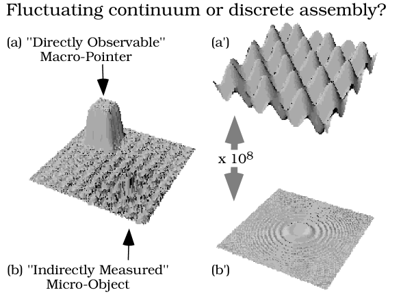
FIG. 1.: A caricature of the observational process. A directly observable quasi–classical pointer, item (a), is coupled to a previously well–isolated elementary constituent, item (b). From the configuration of (a), and knowledge of the coupling, information can be deduced about the unseen system (b). In nature, (a) can exhibit gross fluctuations which are generally interpreted as indicating a discrete foundation for the quantum world. However, given the vast leap in scale, one can equally well imagine theories where the observable reality is described by a coarse–grained continuum field, see the notional magnifications at (a^′) and (b^′). Then the observational process might be traced to collective correlations and fluctuations in the values of this field as a whole — without any assumption of fundamental discreteness. The key to such a continuum theory must lie in the chosen prescription for coarse–graining. It is here that elements of quantum theory might be brought into direct correspondence with the observable reality, so to bypass any need for an observer.

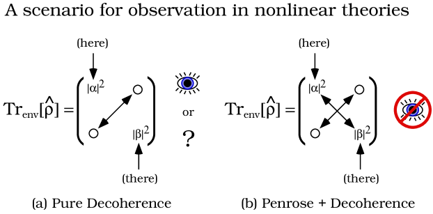
FIG. 2.: In a nonlinear theory one must explain transition probabilities without postulating them, so that a theory of individual events is the natural goal. The existing theory of environmental decoherence provides a route to justify the values these take, see panel (a). There the effect of the environment is to decohere the reduced density matrix into diagonal form in the Zurek pointer basis (Zurek 1981, 1982, 1991). However, because linear interactions entangle states there is no way to cross–couple the diagonal entries. If we invoke the Penrose scenario (1993), of an emergent gravitational instability, one might hope to reduce the remaining terms in stochastic fashion (cf. Diósi 1989). This scenario is advanced as a guide to locating candidate nonlinear terms.

FIG. 3.: On a cosmic scale the Copenhagen theory is open. A simple example is the Newtonian cosmology fixed by a scalar massive field, with no other sources present. Some external agent, here represented by an eyeball, must intervene to define what happens through the act of observation, panel (a). In the Schrödinger theory the act of observation is to be replaced by a dynamic localizing self–potential, panel (b). In that case the cosmology is closed, and one may legitimately pursue an objective interpretation.

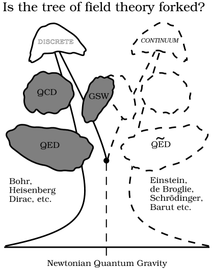
FIG. 4.: Since there are two consistent ways to include gravitation, and these differ in their philosophy, physical interpretation, equations, and predictions, we may view Newtonian quantum gravity as a critical fork which divides quantum field theories into two classes. One is a discrete theory, the other a continuum theory. Since quantum gravity is not directly testable we must seek indirect tests of the continuum alternative. The key issue must be self–energy, and whether a consistent nonlinear treatment is possible for the remaining physical interactions. The self–field quantum electrodynamics of Barut (1990), here labelled as $\tilde{\rm QED}$, is an obvious candidate theory for deeper studies in unification.

FIG. 5.: Universal functions for (a) the gravitational ground state, and (b) ground–state self–potential; and (c) the first excited–state, and (d) excited–state self–potential. A cosmic scale is set for each wave–packet, and no external observer is needed. Thus the gravitational Schrödinger equation exhibits a closed Newtonian quantum cosmology.