LBL-35973

Quantum Electrodynamics at Large Distances III: Verification of Pole Factorization and the Correspondence Principle

Takahiro Kawai

Research Institute for Mathematical Sciences
Kyoto University
Kyoto 606-01 JAPAN
Henry P. Stapp

Lawrence Berkeley Laboratory
University of California
Berkeley, California 94720

In two companion papers it was shown how to separate out from a scattering function in quantum electrodynamics a distinguished part that meets the correspondence-principle and pole-factorization requirements. The integrals that define the terms of the remainder are here shown to have singularities on the pertinent Landau singularity surface that are weaker than those of the distinguished part. These remainder terms therefore vanish, relative to the distinguished term, in the appropriate macroscopic limits. This shows, in each order of the perturbative expansion, that quantum electrodynamics does indeed satisfy the pole-factorization and correspondence-principle requirements in the case treated here. It also demonstrates the efficacy of the computational techniques developed here to calculate the consequences of the principles of quantum electrodynamics in the macroscopic and mesoscopic regimes.

Disclaimer

This document was prepared as an account for work sponsored by the United States Government. Neither the United States Government nor any agency thereof, nor The Regents of the University of California, nor any of their employees, makes any warranty, express or implied, or assumes any legal liability or responsibility for the accuracy, completeness, or usefulness of any information, apparatus, product, or process disclosed, or represents that its use would not infringe privately owned rights. Reference herein to any specific commercial products process, or service by its trade name, trademark, manufacturer, or otherwise, does not necessarily constitute or imply its endorsement, recommendation, or favoring by the United States Government or any agency thereof, or The Regents of the University of California. The views and opinions of authors expressed herein do not necessarily state or reflect those of the United States Government or any agency thereof of The Regents of the University of California and shall not be used for advertising or product endorsement purposes.

Lawrence Berkeley Laboratory is an equal opportunity employer.

1. Introduction

In papers I¹ and II² we examined the functions $F(g)$ associated with the infinite set of graphs $\{g\}$ obtained by dressing a simple triangle graph $G$ with soft photons in all possible ways. A distinguished set of contribution to these functions $F(g)$ was singled out and called “dominant” because these contributions were expected to dominate the macroscopic behaviour of the scattering functions. Each of these distinguished parts was shown to be well defined, and to have a singularity of the form $\log\varphi$ on the (Landau-Nakanishi) triangle-diagram singularity surface $\varphi=0$. This form $\log\varphi$ agrees with the form of the singularity of the original Feynman function $F(G)$ on $\varphi=0$, and it produces the same kind of large-distance fall-off. Moreover, these dominant contributions yield (exactly once) every term in the perturbative expansion of the triangle-diagram version of the pole-factorization property

$$\mbox{Disc}F^{\prime}|_{\varphi=0}=F^{\prime}_{1}F^{\prime}_{2}F^{\prime}_{3}.$$

The left-hand side of this equation represents value at $\varphi=0$ of the discontinuity across the surface $\varphi=0$ of the function $F^{\prime}$ that is obtained by omitting the contributions from the “classical” photons. These latter contributions are supplied by the unitary operator $U(L)$ — after the transformation to coordinate space. Consequently, the discontinuity formula given above entails that the contributions from these “dominant” terms give just the classical-type large-distance behaviour demanded by the correspondence principle: the rate of fall-off at large distances is exactly what follows from the classical concept of three stable charged particles, each moving from one scattering region to another, and the electromagnetic field generated by $U(L)$ is exactly the quantum analog of the classical electromagnetic field generated by the motions of these three charged particles. In the present article we shall show that, in each order of the perturbation expansion, the terms of the remainder give no contributions to the discontinuity defined above. Consequently, these “non-dominant” terms give no contribution to the leading term in the the asymptotic large-distance behaviour, and hence the correspondence-principle requirement is satisfied.

In section 2 we examine the simplest example, namely the triangle graph $G$ dressed with one internal soft photon. The remainder part is separated into a sum of terms. For some terms the weakening of the singularity on the surface $\varphi=0$ is associated with the topological complexity of the graph that represents this term, namely its non-separability: cutting the graph at the three $*$ lines associated with the three Feynman-denominator poles does not separate the graph into three disjoint parts. This means that the integration over the momenta of the internal photons tends to shift the position of the singularity, and hence weaken it. For the remaining terms the weakening of the singularity on $\varphi=0$ is due to the replacement of one or more of the three pole singularities $(p_{s}^{2}-m^{2})^{-1}$ of the integrand by a pair of logarithmic singularities: this replacement of the pole singularities in the integrand by logarithmic singularities likewise leads to a weakening of the singularity of the integral on $\varphi=0$.

Our problems here are first to show that these reductions in the degree of the singularity on $\varphi=0$, which emerge easily within our formalism in this simple one-photon example, hold for every $g$ obtained by dressing the triangle graph $G$ with soft photons, and second to show that the weakening of the singularity is, in every case, a weakening by at least one full power of $\varphi$, up to a prescribed finite number of powers of $\log\varphi$ that increases linearly with the number of photons, and hence with powers of the coupling constant. This strong result means that the validity of the correspondence–principle in the large–scale limit, which is established here at each order of the perturbative expansion, cannot be upset by an accumulation of powers of $(\log\varphi)^{n}$ that leads to a singularity of the form $\varphi^{-\beta}$, where $\beta$ is of the order of the fine-structure constant $(\sim 1/137)$. Accumulations of this kind occur often in field theories. The appearance of the fine-structure constant in the exponent arises from the fact that usually, just as in our case, the number of powers of $\log\varphi$ is linearly tied to the number of powers of the fine-structure constant. We have not studied, in our case, the numerical factors that multiply the terms of the remainder, except to show that they are all finite. Hence we can make here no claim pertaining to meaningfulness of the infinite sum in our case: we plan to examine this question later.

To establish our general conclusions we need two auxiliarly results. The first is a geometric property concerning the structure of the Landau-Nakanishi surface. It is proved in section 3. The second pertains to several singular integrals. The needed computation is performed in section 4. The required properties of the various intergrals are then proved in sections 5, 6, and 7.

2. Examination of non-dominant singularities for the one-photon case.

Let us consider the contributions associated with the graph $g$ shown in Figure ^fig1).

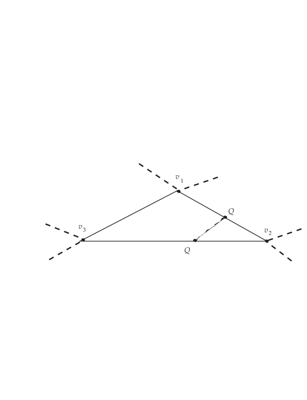
Figure 1: A graph $g$ representing a soft-photon correction to a hard-photon triangle-diagram process $G$. The letters Q near the ends of the wiggly line that represents the soft photon indicate that this particle is coupled to the charged particle through the “quantum” part of the full quantum-electrodynamical coupling.

In references 1 and 2 we showed how to separate the contribution represented by the graph of Fig. 1 into a meromorphic part consisting of a sum of the four terms represented by the the four $*$ graphs of Figure ^fig2) , plus a “non-meromorphic” part.

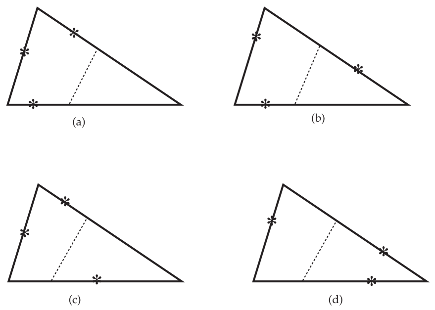
Figure 2: Four $*$ graphs representing the four terms in the meromorphic part of the function represented by the graph in fig. 1. These four terms arise from a decomposition of the meromorphic parts associated with each of the three sides of the triangle into poles times residues. The $*$ lines represent Feynman-denominator poles. The other charged-particle lines represent residue factors.

The term associated with the graph $a$ of Figure 2 is separable, and is classified as dominant. The associated function $F_{a}$ is given by (4.1) and (4.3) of Ref. 1, and has a logarithmic singularity along the Landau surface $\varphi=0$. We also claimed there that the other three terms in the meromorphic part are are infrared finite, and have weaker singularities along the Landau surface $\varphi=0$. In the following subsection we verify this claim for the case of the function $F_{b}$ associated with graph (b) of Fig. 2. The other two cases, $c$ and $d$, can be treated similarly.

2.i. The contribution from a one-photon nonseparable meromorphic part.

The function $F_{b}$ was given in (4.4) of Ref. 1:

$$\eqalignno{F_{b}&=\int{d^{4}p\over(2\pi)^{4}}\int^{\delta}_{0}2rdr\int{d^{4}\Omega\over(2\pi)^{4}}\ \ {i\delta(\Omega^{2}_{0}+\vec{\Omega}^{2}-1)\over\Omega^{2}+i0}\cr&\Tr\Bigg{\{}{i(/{p}+m)\over p^{2}-m^{2}}V_{1}\bigg{(}{(2p_{i\mu}+2r\Omega_{\mu})\Omega^{2}(2p_{1}\Omega+2r\Omega^{2})^{-1}-/{\Omega}\gamma_{\mu}\over 2p_{1}\Omega+r\Omega^{2}}\bigg{)}\cr&\times{(/{p}_{1}+r/{\Omega}+m)\over(p_{1}+r\Omega)^{2}-m^{2}}V_{2}\cr&\times\bigg{(}{2p_{2\mu}\Omega^{2}(2p_{2}\Omega)-\gamma_{\mu}/{\Omega}\over 2p_{2}\Omega+r\Omega^{2}}\bigg{)}{(/{p}_{2}+m)\over p^{2}_{2}-m}V_{3}\bigg{\}}&(2.ii.1)\cr}$$

It was shown in Ref. 2 that we can distort the $\Omega$-contour so that Im$\Omega^{2}>0$ at $\Omega^{2}=0$, and Im$p_{j}\Omega>0\ (j=1,2)$ at $p_{j}\Omega=0$. Then, except for three pole-factors $p^{2}-m^{2},(p_{1}+r\Omega)^{2}-m^{2}$ and $p^{2}_{2}-m^{2}$, each denominator of the integrand of $F_{b}$ is different from zero.

The $r$-integration $\int^{\delta}_{0}rdr/[(p_{1}+r\Omega)^{2}-m^{2}$] can be explicitly performed, and when $p_{1}\Omega\neq 0$ its dominant singularity along $p^{2}_{1}=m^{2}$ is

$$-{(p^{2}_{1}-m^{2})\log(p^{2}_{1}-m^{2})\over 4(p_{1}\Omega)^{2}}.$$

Combining this singularity, instead of the ordinary pole $1/(p^{2}_{1}-m^{2})$, with the other two poles, i.e., $1/(p^{2}-m^{2})$ and $1/(p^{2}_{2}-m^{2})$, we perform the $p$-integration and find a singularity $A(q,\Omega)\varphi(q)^{2}\log\varphi(q)$, with $A$ being analytic. Performing the $\Omega$-integration along the compact distorted contour, the dominant singularity of $F_{b}$ is $\varphi^{2}\log\varphi$.

Essentially the same argument covers the case where one of the two meromorphic parts is due to a $C$-coupling. Then the factor $rdr$ becomes simply $dr$, and the singularity becomes $\varphi\log\varphi$.

2.ii. The contribution from a pair of non-meromorphic parts arising from one photon.

The contribution of $I$ in (4.6) in Ref. 1 to the amplitude is

$$\eqalignno{F&=\int_{|\Omega|=1}{d^{4}\Omega\over\Omega^{2}+i0}\int^{\delta}_{0}{dr\over r}\int d^{4}p_{3}{1\over p^{2}_{3}-m^{2}+i0}\log{(q_{1}+p_{3}+r\Omega)^{2}-m^{2}+i0\over(q_{1}+p_{3})^{2}-m^{2}+i0}\cr&\times\log{(p_{3}-q_{3}-r\Omega)^{2}-m^{2}+i0\over(p_{3}-q_{3})^{2}-m^{2}+i0},&(2.ii.1)\cr}$$

with the $p_{i}$ defined as in Fig. 1 of ref.2. Here the $\Omega$-contour is deformed so that Im$\Omega^{2}>0$ and Im$p_{j}\Omega>0$ (j=1,2). Performing the $p_{3}$-integration we find

$$\eqalignno{\int_{|\Omega|=1}{d^{4}\Omega\over\Omega^{2}+i0}&\int^{\delta}_{0}{dr\over r}(G(q_{1}+r\Omega,q_{3}+r\Omega)\cr&-G(q_{1}+r\Omega,q_{3})-G(q_{1},q_{3}+r\Omega)+G(q_{1},q_{2})).&(2.ii.2)\cr}$$

where

$$G(q_{1},q_{2})=\varphi(q_{1},q_{2})^{2}\log(\varphi(q_{1},q_{2})+i0).$$

Since

$$\eqalignno{(\partial/\partial r)\varphi(q_{1}+r\Omega,q_{3}+r\Omega)&=(\partial\varphi/\partial q_{1}+\partial\varphi/\partial q_{3})\cdot\Omega\cr&=(\alpha_{1}\rho_{1}+\alpha_{2}\rho_{2})\cdot\Omega=-\alpha_{3}p_{s}\cdot\Omega\neq 0\cr}$$

holds by the Landau equation, we can find non-vanishing functions $a(q_{1},q_{3},r,\Omega)$ and $b(q_{1},q_{3})$ for which

$$\varphi(q_{1}+r\Omega,q_{3}+r\Omega)=a(q_{1},q_{3},r,\Omega)(r-b(q_{1},q_{3})\varphi(q_{1}+r\Omega,q_{3}))$$

holds (Cf.$\S$ 3 below). Similar decompositions hold also for $\varphi(q_{1}+r\Omega,q_{2})$ and $\varphi(q_{1},q_{2}+r\Omega)$. Hence application of the results in $\S$ 4 below to $\int^{\delta}_{0}{dr\over r}(G(q_{1}+r\Omega,q_{3}+r\Omega)-G(q_{1},q_{3}))$ etc. entails that the $r$-integration in (2.ii.2) produces a singularity of the form $\varphi(q_{1},q_{3})^{2}(\log(\varphi(q_{1},q_{3})+i0)^{2}$ near $\varphi=0$. Since the $\Omega$-integration (along a suitably detoured path) is over the compact set, $F$ itself behaves as $\varphi^{2}(\log(\varphi+i0))^{2}.$

2.iii. The contribution from a coupling of a non-meromorphic part with either a meromorphic part or a $C$-part.

If a meromorphic part is coupled with a non-meromorphic part, the RHS of (2.ii.1) is replaced by an integral of the following form:

$$\eqalignno{\int_{|\Omega|=1}{d^{4}\Omega\over\Omega^{2}+i0}&\int^{\delta}_{0}dr\int d^{4}p_{3}{1\over p^{2}_{3}-m^{2}+i0}\log{(q_{1}+p_{3}+r\Omega)^{2}-m^{2}+i0\over(q_{1}+p_{3})^{2}-m^{2}+i0}\cr&{1\over(p_{3}-q_{3})^{2}-m^{2}+i0}\ \ {1\over 2(p_{3}-q_{3})\Omega+r\Omega^{2}+i0}.&(2.iii.1)\cr}$$

By deforming the $\Omega$-contour, in the manner specified in ref. 2, so that Im$\Omega^{2}>0$ and Im$p_{j}\Omega>0(j=1,2)$ [with $p_{1}=q_{1}+p_{3},p_{2}=p_{3}-q_{3}$], we find the singularity of this integral near $\varphi(q_{1},q_{3})=0$ is $\varphi\log(\varphi+i0)$, as there is no potentially divergent factor $1/r$.

If the meromorphic part is replaced by a $C$-term, then the dominant singularity is given by an integral similar to (2.iii.1) but with the replacement of the residue factor $1/(2(p_{3}-q_{3})\Omega+r\Omega^{2})$ by $1/r(p_{3}-q_{3})\Omega$. Hence a potentially divergent factor $1/r$ arises. But this problem is circumvented by combining the singularity originating from $\log((q_{1}+p_{3}+r\Omega)^{2}-m^{2}+i0)$ and that from $\log((q_{1}+p_{3})^{2}-m^{2}+i0)$; the results in $\S$ 4 show, with a reasoning similar to (but simpler than) that in $\S$ 2.ii, that the resulting singularity is $\varphi(\log(\varphi+i0))^{2}$.

3. A normalization of the function defining a Landau surface.

The purpose of this section is to prove the following lemma, which is an adaptation of the implicit function theorem (or the Weierstrass preparation theorem in the theory of holomorphic functions of several variables) to the Landau surface shifted by a vector $\Delta$ determined by photons that bridge star lines. (cf.$\S$ 11. of Ref. 1.). Here and in what follows, $(r_{1},...,r_{n})$ denotes a nested set of polar coordinates introduced in Ref. 1, $\S$5.

Lemma 3.1 Let $\varphi(q)$ denote a defining function of the Landau surface for the triangle diagram and let $\hat{q}$ be a point on the surface. Let $i$ be the smallest $j$ such that $j$ identifies a bridge photon line. (A bridge photon line is a photon line that has meromorphic couplings on both ends and that completes — via the rules defined below Eqn. (2)of ref. 2 — to a closed photon loop that passes along at least one star line.) Then on a sufficiently small neighborhood of $q_{0}$ and for sufficiently small $\rho_{i}=r_{1}\cdots r_{i}$ there exist non-vanishing holomorphic functions $B(q,\rho_{i},k^{\prime}/\rho_{i})$ and $C(q,k^{\prime}/\rho_{i})$ such that

$$\varphi(q-\Delta)=B(q,\rho_{i},k^{\prime}/\rho_{i})(\rho_{i}-\varphi(q)/C(q,k^{\prime}/\rho_{i}))$$

holds, where $k^{\prime}$ denotes the collection of bridge lines.

Proof. Since $i$ is the first bridge photon line, any bridge photon line $k_{\ell}$ has the form $k_{\ell}=\rho_{i}r_{i+1}\cdots r_{\ell}\Omega_{\ell}$. Hence $k^{\prime}/\rho_{i}$ is actually independent of $\rho_{i}$. Furthermore, as is shown at the beginning of section 5 ((5.1)),$\partial\varphi(q-\Delta)/\partial\rho_{i}|_{\rho_{i}=0}\neq 0$ holds. Hence the Weierstrass preparation theorem guarantees the local and unique existence of a non-vanishing holomorphic function $B(q,\rho_{i},k^{\prime}/\rho_{i})$, and a holomorphic function $R(q,k^{\prime}/\rho_{i})$, which vanishes for $q_{i}=q_{0}$, for which the following holds:

$$\varphi(q-\Delta)=B(q,\rho_{i},k^{\prime}/\rho_{i})(\rho_{i}-R(q,k^{\prime}/\rho_{i}))$$

Setting $\rho_{i}=0$ in (3.2) we find

$$\varphi(q)=B(q,0,k^{\prime}/\rho_{i})(-R(q,k^{\prime}/\rho_{i}),$$

that is,

$$R(q,k^{\prime}/\rho_{i})=\varphi(q)/(-B(q,0,k^{\prime}/\rho_{i})).$$

Hence by choosing $C(q,k^{\prime}/\rho_{i})=-B(q,0,k^{\prime}/\rho_{i})$ we obtain (3.1).

4. Some auxiliary integrals.

The purpose of this section is to find an explicit form of the singularities of several integrals that we encounter in dealing with infrared problems. The simplest example of this sort is the following integral $I(t)$:

$$I(t)=\int^{\delta}_{0}[\log(r+t+i0)-\log(t+i0)]dr/r,\ \ (\delta>0).$$

In spite of the divergence factor $1/r$, $I(t)$ is well defined as a (hyper) function of $t$. In order to see this, it suffices to decompose $I(t)$ as

$$\int^{t/2}_{0}(\log(r+t)-\log t)dr/r+\int^{\delta}_{t/2}(\log(r+t)-\log t)dr/r$$

with $Im\ t>0$: the well-definedness of the second integral is clear, while the fact that

$$\log(r+t)-\log t=\log(1+{r\over t})\sim{r\over t}$$

holds in the domain of integration of the first integral entails its well-definedness. Furthermore $I(t)$ (thus seen to be well-defined) satisfies the following ordinary differential equation:

$$t{d\over dt}I(t)=\log(t+i0)-\log(t+\delta+i0).$$

Hence $(t{d\over dt})^{2}$ is holomorphic near $t=0$. Then it follows from the general theory of ordinary differential equations that $I(t)$ has the form

$$C_{2}(\log(t+i0))^{2}+C_{1}(\log(t+i0))+h(t),$$

where $C_{1}$ and $C_{2}$ are constants and $h(t)$ is holomorphic near $t=0$. Furthermore, by substituting (4.2) into (4.1) and comparing the coefficients of singular terms at $t=0$, we find $C_{2}=1/2$.

This computation can be generalized as follows:

Proposition 4.1. Let $J(\alpha,j;t)\ (\alpha\neq 0,1,2,\cdots;j\geq 1)$ denote the following integral:

$$\int^{\delta=\rho_{0}}_{0}{d\rho_{1}\over\rho_{1}}\int^{\rho_{1}}_{0}{d\rho_{2}\over\rho_{2}}\cdots\int^{\rho_{j-2}}_{0}{d\rho_{j-1}\over\rho_{j-1}}\int^{\rho_{j-1}}_{0}(t+\rho_{j}+i0)^{\alpha}d\rho_{j}.$$

Then the singularity of $J(\alpha,j;t)$ near $t=0$ is of the following form with some constants $C_{\ell}\ (\ell=0,\cdots,j-1)$:

$$\Bigg{\{}\matrix{(t+i0)^{\alpha+1}(\sum^{j-1}_{\ell=0}C_{\ell}(\log(t+i0))^{\ell}),&\hbox{if}\ \alpha\neq-1\cr\sum^{j-1}_{\ell=0}C_{\ell}(\log(t+i0))^{\ell+1},&\hbox{if}\ \alpha=-1}.$$

Remark 4.1. If $\alpha$ is a non-negative integer, the integral $J(\alpha,j;t)$ is not singular at $t=0$.

Proof of Proposition 4.1. The well-definedness can be verified by the same method as was used for the above example $I(t)$. To find its singularity structure, we again make use of an ordinary differential equation as follows:

$$\eqalignno{&(t{d\over dt}-(\alpha+1))J(\alpha,j;t)=\left(t{d\over dt}-(\alpha+1)\right)\int^{\delta}_{0}{d\rho_{1}\over\rho_{1}}\int^{\rho_{1}}_{0}{d\rho_{2}\over\rho_{2}}\cdots\cr&\int^{\rho_{j-2}}_{0}{d\rho_{j-1}\over\rho_{j-1}}((t+\rho_{j-1}+i0)^{\alpha+1}-(t+i0)^{\alpha+1})/(\alpha+1)\cr&=\int^{\delta}_{0}{d\rho_{1}\over\rho_{1}}\int^{\rho_{1}}_{0}{d\rho_{2}\over\rho_{2}}\cdots\int_{0}^{\rho_{j-2}}{d\rho_{j-1}\over\rho_{j-1}}(t(t+\rho_{j-1}+i0)^{\alpha}-(t+\rho_{j-1}+i0)^{\alpha+1})\cr&=-\int^{\delta}_{0}{d\rho_{1}\over\rho_{1}}\int^{\rho_{1}}_{0}{d\rho_{2}\over\rho_{2}}\cdots\int^{\rho_{j-2}}_{0}(t+\rho_{j-1}+i0)^{\alpha}d\rho_{j-1}=-J(\alpha,j-1;t)(j\geq 2).\cr}$$

Repeating this computation, we finally obtain

$$(t{d\over dt}-(\alpha+1))^{j-1}J(\alpha,j;t)=(-1)^{j-1}\int^{\delta}_{0}(t+\rho_{1})^{\alpha}d\rho_{1},$$

and hence we find $(t{d\over dt}-(\alpha+1))^{j}J(\alpha,j;t)$ is holomorphic near $t=0$. Again, by using the general theory of ordinary differential equations, we obtain the required formula (4.3).

Remark 4.2. Although we do not need the exact values of $C_{\ell}$’s, we note that $C_{j-1}$ in (4.3) is simply given by $(-1)^{j-2}/(j-1)!(\alpha+1)$ if $\alpha\neq-1$. In order to find this value it suffices to insert (4.3) into the recurrence relation $(td/dt-(\alpha+1))J(\alpha,j;t)=-J(\alpha,j-1;t)$ and use the trivial relation

$$\eqalignno{\left(t{d\over dt}-(\alpha+1)\right)J(\alpha,2;t)&=-\int^{\delta}_{0}(t+\rho_{1}+i0)^{\alpha}d\rho_{1}\cr&=((t+i0)^{\alpha+1}/(\alpha+1))-((t+\delta+i0)^{\alpha+1}/(\alpha+1))\cr}$$

as the starting point of the induction. Similarly $C_{j-1}$ for $\alpha=-1$ is equal to $(-1)^{j}/j!$. The coefficient of the most singular term can be similarly computed explicitly for the integrals to be dealt with in subsequent propositions.

The following modification of Proposition 4.1 is often effective in actual computations.

Proposition 4.2. (i) Let $K(\alpha,j;t)\ (\alpha\neq 0,1,\cdots;j\geq 1)$ denote the following integral:

$$\int^{\delta}_{0}{d\rho_{1}\over\rho_{1}}\int^{\rho_{1}}_{0}{d\rho_{2}\over\rho_{2}}\cdots\int^{\rho_{j}-2}_{0}{d\rho_{j-1}\over\rho_{j-1}}\int^{\rho_{j-1}}_{0}\rho_{j}(t+\rho_{j}+i0)^{\alpha}d\rho_{j}.$$

Then its singularity near $t=0$ is of the following form for some constants $C_{\ell}(\ell=0,\cdots,j-1)$:

$$\Bigg{\{}\matrix{(t+i0)^{\alpha+2}\left(\sum^{j-1}_{\ell=0}C_{\ell}(\log(t+i0))^{\ell}\right)&\hbox{if}\ \alpha\neq-1,-2\cr t^{\alpha+2}\left(\sum^{j-1}_{\ell=0}C_{\ell}(\log(t+i0))^{\ell+1}\right)&\hbox{if}\ \alpha=-1\ {\hbox{or}}\ -2}.$$

(ii) Let $n$ be a non-negative integer and let $I(n,j;t)(j\geq 1)$ denote the following integral:

$$\int^{\delta}_{0}{d\rho_{1}\over\rho_{1}}\int^{\rho_{1}}_{0}{d\rho_{2}\over\rho_{2}}\cdots\int^{\rho_{j-2}}_{0}{d\rho_{j-1}\over\rho_{j-1}}\int^{\rho_{j-1}}_{0}(t+\rho_{j})^{n}\log(t+\rho_{j}+i0)d\rho_{j}.$$

Then its singularity near $t=0$ is of the following form with some constants $C_{\ell}(\ell=0,\cdots,j-1)$:

$$t^{n+1}\left(\sum^{j-1}_{\ell=0}C_{\ell}(\log(t+i0))^{\ell+1}\right).$$

(iii) Let $\widetilde{I}(n,j;t)(n$; a non-negative integer, and $j\geq 1$) denote the following integral:

$$\int^{\delta}_{0}{d\rho_{1}\over\rho_{1}}\int^{\rho_{1}}_{0}{d\rho_{2}\over\rho_{2}}\cdots\int^{\rho_{j-2}}_{0}{d\rho_{j-1}\over\rho_{j-1}}\int^{\rho_{j-1}}_{0}\rho_{j}(t+\rho_{j})^{n}\log(t+\rho_{j}+i0)d\rho_{j}.$$

Then its singularity near $t=0$ is of the following form with some constants $C_{\ell}(\ell=0,\cdots,j-1)$:

$$t^{n+2}\left(\sum^{j-1}_{\ell=0}C_{\ell}(\log(t+i0))^{\ell+1}\right).$$

Proof. Since $\rho_{j}(t+\rho_{j})^{\alpha}=(t+\rho_{j})^{\alpha+1}-t(t+\rho_{j})^{\alpha}$, (i) and (iii) follow respectively from Proposition 4.1 and from (ii) above. Hence it remains to prove (ii). Since

$${d^{n+1}\over dt^{n+1}}\left((t+\rho_{j})^{n}\log(t+\rho_{j}+i0)\right)={n!\over t+\rho_{j}+i0}+P_{n},$$

where $P_{n}$ is a polynomial of $(t+\rho_{j})$, Remark 4.1, entails that

$${d^{n+1}\over dt^{n+1}}I(n,j;t)+n!J(-1,j;t)+h(t)$$

holds with a holomorphic function $h(t)$. On the other hand, near $t=0$ a straightforward computation shows

$$\int^{t}dt\ t^{n}(\log(t+i0))^{m}={t^{n+1}\over n+1}\sum^{m}_{r=0}{(-1)^{r}m!(\log(t+i0)^{m-r}\over(m-r)!(n+1)^{r}}$$

holds for non-negative integers $n$, and $m\neg 1$. Combining (4.7) and Proposition 4.1, we use (4.8) repeatedly to find (4.5). We also note that Remark 4.2 entails $C_{j-1}=(-1)^{j}/j!(n+1)$ in this case.

The following proposition is a key result of this section.

Proposition 4.3. Let $I(t)$ denote the following integral (4.9), where $e_{j}\ (j=1,2,\cdots,n)$ is a non-negative integer:

$$\int^{\delta}_{0}r^{e_{1}}_{1}dr_{1}\int^{1}_{0}r_{2}^{e_{2}}dr_{2}\cdots\int^{1}_{0}r_{n}^{e_{n}}dr_{n}\log(t+r_{1}\cdots r_{n}+i0).$$

Then its singularity near $t=0$ is a sum of finitely many terms of the form

$$Ct^{N}(\log(t+i0))^{m}$$

with a constant $C$ and positive integers $N(\geq min\ \ e_{j}+1)$ and $m(\leq n)$.

Proof. First of all, let us re-scale the parameter $r_{1}$ and the variable $t$ as follows:

$$r_{1}=\delta r^{\prime}_{1},\ \ t=\delta s$$

Then $I$ becomes

$$\delta^{-e_{1}-1}\int^{1}_{0}(r^{\prime}_{1})^{e_{1}}dr^{\prime}_{1}\int^{1}_{0}r_{2}^{e_{2}}dr_{2}\cdots\int^{1}_{0}r_{n}^{e_{n}}dr_{n}(\log(s+r^{\prime}_{1}r_{2}\cdots r_{n})+\log\delta).$$

The contribution from $\log\delta$ in (4.11) is a finite constant. Thus we may assume from the first that $\delta=1$. Then the roles of $r_{j}^{\prime}s$ in (4.9) are uniform, and hence we may re-number the index $j$ so that

$$e_{1}\geq e_{2}\geq\cdots\geq e_{n}.$$

Let us introduce new variables $\sigma_{j}$ by

$$\sigma_{1}=r_{1},\ \ \sigma_{2}=r_{1}r_{2},\cdots,\ \sigma_{n}=r_{1}\cdots r_{n}.$$

The integral $I$ (with $\delta=1$) can be now expressed as

$$\int^{1}_{0}{\sigma_{1}^{d_{1}}\over\sigma_{1}}d\sigma_{1}\int^{\sigma_{1}}_{0}{\sigma_{2}^{d_{2}}\over\sigma_{2}}d\sigma_{2}\cdots\int^{\sigma_{n-2}}_{0}{\sigma_{n-1}^{d_{n-1}}\over\sigma_{n-1}}d\sigma_{n-1}\int^{\sigma_{n-1}}_{0}\sigma_{n}^{e_{n}}d\sigma_{n}\log(t+\sigma_{n}+i0),$$

where $d_{j}=e_{j}-e_{j+1}$. The number $d_{j}$ is nonnegative by (4.12), and this non-negativity makes our reasoning much simpler: that is why we re-numbered the index $j$.

The first integration in (4.14), i.e. $\int^{\sigma_{n-1}}_{0}\sigma^{e_{n}}_{n}d\sigma_{n}\log(t+\sigma_{n}+i0)$, can be done in a straightforward manner: using the identity $\sigma^{e}=\sum^{e}_{j=0}c_{j}t^{j}(t+\sigma)^{e-j}$, where $c_{j}$ is some constant, we find it is a sum of terms of the form

$$\eqalignno{Ct^{j}\big{\{}(t&+\sigma_{n-1})^{e_{n}-j+1}\log(t+\sigma_{n-1}+i0)\cr&-t^{e_{n}-j+1}\log(t+i0)\big{\}}&(4.15)\cr}$$

and polynomials of the form

$$C^{\prime}t^{j}\{(t+\sigma_{n-1})^{e_{n}-j+1}-t^{e_{n}-j+1}\},$$

where $C$ and $C^{\prime}$ are some constants.

If $d_{n-1}\geq 1$, the same computation can be done for the second integration (4.14). In this case we do not need to combine the first term and the second term in (4.15). That is, we perform the integration of these terms separately. If $d_{n-1}$ is equal to $0$, we first define an integral $J$ by

$$\int_{0}^{1}{\sigma^{d_{1}}\over\sigma_{1}}d\sigma_{1}\int^{\sigma_{1}}_{0}{\sigma_{2}^{d_{2}}\over\sigma_{2}}d\sigma_{2}\cdots\int^{\sigma_{n-2}}_{0}{d\sigma_{n-1}\over\sigma_{n-1}}\{(t+\sigma_{n-1})^{\alpha}\log(t+\sigma_{n-1}+i0)-t^{\alpha}\log(t+i0)\},$$

where $\alpha=e_{n}-j+1$ is a positive integer. Then we have

$$\eqalignno{(t{d\over dt}&-\alpha)J(t)\cr&=\int^{1}_{0}{\sigma_{1}^{d_{1}}\over\sigma_{1}}d\sigma_{1}\int^{\sigma_{1}}_{0}{\sigma_{2}^{d_{2}}\over\sigma_{2}}d\sigma_{2}\cdots\int^{\sigma_{n-2}}_{0}d\sigma_{n-1}\big{\{}-\alpha(t+\sigma_{n-1})^{\alpha-1}\log(t+\sigma_{n-1}+i0)\cr&+((t+\sigma_{n-1})^{\alpha-1}-t^{\alpha-1})/\sigma_{n-1}\big{\}}\cr}$$

Since the contribution from $((t+\sigma_{n-1})^{\alpha-1}-t^{\alpha-1})/\sigma_{n-1}$ is finite and analytic in $t$ (actually a polynomial), the main contribution to $J(t)$ is from $-\alpha(t+\sigma_{n-1})^{\alpha-1}\log(t+\sigma_{n-1}+i0)$. But this is the same integral discussed at the first step. Repeating this procedure we finally find that $I$ has the form $\sum^{e_{n}}_{j=0}t^{j}I_{j}$, where $I_{j}$ satisfies the following equation:

$$\prod^{n(j)}_{\ell=1}(t{d\over dt}-\alpha_{\ell}(j))I_{j}(t)=\sum_{k}(C_{k}\log(t+i0)+C^{\prime}_{k})t^{k}+A,$$

where $A$ is analytic at $t=0$. Here $n(j)\leq n-1,\ \ \alpha_{\ell}(j)$ is an integer $\geq e_{n}-j+1,k$ ranges over a finite subset of integers $\geq e_{n}-j+1$, and $C_{k}$ and $C^{\prime}_{k}$ are constants. As a solution of the equation (4.17), $I_{j}(t)$ [modulo a function analytic at $t=0$] is a sum of terms of the form

$$Ct^{N}(\log(t+i0))^{m}$$

with a constant $C$ and integers $N\geq e_{n}-j+1$ and $m\leq n$. Thus $I(t)$ consists of terms of the required form (4.10). Note that min $e_{j}=e_{n}$ by the re-numbering of the index $j$.

Remark 4.3. (i) If log $(t+r_{1}...r_{n}+i0)$ in (4.9) is replaced by $(t+r_{1}...r_{n}+i0)^{\alpha}$ ($\alpha$: non-integer), the resulting integral is a finite sum of terms of the form

$$Ct^{\alpha+e}(\log(t+i0))^{m}$$

with an integer $e\geq\min e_{j}+1$ and a non-negative integer $m\leq n-1$. If $\alpha=-1$, then the condition on $e$ is the same as above but the condition on $m$ is replaced by $m\leq n$.

(ii) Let $a(r^{\prime})$ be an analytic function of $r^{\prime}=(r^{\prime}_{1}...,r^{\prime}_{n}$), in a closed “cube” $C=[\epsilon,1]\times...\times[\epsilon,1](\epsilon>0)$. Then the following integral $F(a)$ has the same singularity as $I(t)$, or a weaker one :

$$F(a)=\int^{1}_{\epsilon}dr^{\prime}_{1}...\int^{1}_{\epsilon}dr^{\prime}_{n^{\prime}}a(r^{\prime})\int^{\epsilon}_{0}r_{1}^{e_{1}}dr_{1}...\int^{\epsilon}_{0}r_{n}^{e_{n}}dr_{n}\log(t+r^{\prime}_{1}...r^{\prime}_{n^{\prime}}...r_{n}+i0).$$

In fact, for $r^{\prime}$ in $C$ we find

$$\eqalignno{&\int^{\epsilon}_{0}r_{1}^{e_{1}}dr_{1}...\int^{\epsilon}_{0}r_{n}^{e_{n}}dr_{n}\log(t+r^{\prime}_{1}...r^{\prime}_{m}r_{1}...r_{n}+i0)\cr=&\int^{\epsilon}_{0}r_{1}^{e_{1}}dr_{1}...\int^{\epsilon}_{0}r_{n}^{e_{n}}dr_{n}\big{\{}\log({t\over r^{\prime}_{1}...r^{\prime}_{m}}+r_{1}...r_{n}+i0)\cr&+\log(r^{\prime}_{1}...r^{\prime}_{m})\big{\}}.\cr}$$

Since the contribution from $\log(r^{\prime}_{1}...r^{\prime}_{m})$ to $F(a)$ is an analytic function, it suffices to consider the contribution from $\log({t\over r^{\prime}_{1}...r^{\prime}_{n^{\prime}}}+r_{1}...r_{n}+i0)$. Proposition 4.3 then tells us that it is a sum of terms of the form

$$\int^{1}_{\epsilon}dr^{\prime}_{1}...\int^{1}_{\epsilon}dr^{\prime}_{n^{\prime}}a(r^{\prime}){t^{N}\over(r^{\prime}_{1}...r^{\prime}_{n^{\prime}})^{N}}(\log(t+i0)-\log(r^{\prime}_{i}...r^{\prime}_{n^{\prime}}))^{m}.$$

Hence the singularity of $F(a)$ near $t=0$ is a sum of terms of the form (4.10). Note that the effect of changing the upper end-point of the integral in (4.9) to $\epsilon$ is absorbed by the harmless change of scaling in $r$ variables and $t$ variable (as was employed at the beginning of the proof of Proposition 4.3), on the condition that $\epsilon$ is a fixed positive constant.

To generalize Proposition 4.3 to the form needed in section 6 we prepare the following Lemma:

Lemma 4.1. Let $L_{m}(t;a)(n=1,2,...;{a}$ a strictly positive constant), denote the following integral:

$$\int^{a}_{0}{(\log w)^{m}\over t+w+i0}dw.$$

Then the singularity structure of $L_{m}$ near $t=0$ is as follows:

$$L_{m}=\sum^{m+1}_{j=1}C_{j}(\log(t+i0))^{j}+h(t)$$

where $C_{j}(j=1,...,m+1)$ are some $a$-dependent constants and $h(t)$ is an a-dependent holomorphic function near $t=0$.

Proof. Since $(\log w)^{m}\theta(w)\theta(a-w)(a>0)$ is well-defined as a product of locally summable functions, the convolution-type integral $L_{m}(t;a)$ is well-defined, and it is a boundary value of a holomorphic function on $\{\Im t>0\}$ near $t=0$. To find out its explicit form (4.18), we first apply an integration by parts:

$$\eqalignno{L_{m}&={\mathop{\lim}_{\kappa\downarrow 0}}\Bigg{\{}-\int^{a}_{\kappa}{m(\log(w+i0))^{m-1}\over w+i0}\log(t+w+i0)dw\cr&+(\log a)^{m}\log(a+t+i0)-(\log(\kappa+i0))^{m}\log(t+\kappa+i0)\Bigg{\}}\cr&={\mathop{\lim}_{\kappa\downarrow 0}}\Bigg{\{}-\int^{a}_{\kappa}{m(\log(w+i0))^{m-1}\over w+i0}\log\left({t+w+i0\over t+i0}\right)dw\cr&-\left(\int^{a}_{\kappa}{m(\log(w+i0))^{m-1}\over w+i0}dw\right)\log(t+i0)-\left(\log(\kappa+i0))^{m}\log(t+\kappa+i0)\right\}\cr&+(\log a)^{m}\log(a+t+i0)\cr&={\mathop{\lim}_{\kappa\downarrow 0}}\Bigg{\{}-\int^{a}_{\kappa}{m(\log(w+i0))^{m-1}\over w+i0}\log\left({t+w+i0\over t+i0}\right)dw\cr&-(\log(\kappa+i0))^{m}\log{t+\kappa+i0\over t+i0}\Bigg{\}}+(\log a)^{m}\log{t+a+i0\over t+i0}&(4.19)\cr}$$

Let us note that, if Im $t>0$,

$$\eqalignno{&(\log(\kappa+i0))^{m}\log{t+\kappa+i0\over t+i0}\cr=&(\log(\kappa+i0))^{m}\left({\kappa+i0\over t+i0}-\half\left({\kappa+i0\over t+i0}\right)^{2}+...\right)\longrightarrow 0\cr}$$

as $\kappa\downarrow 0$. Hence we obtain

$$L_{m}=M_{m}-(\log a)^{m}\log(t+i0)+(\log a)^{m}\log(t+a+i0),$$

where

$$M_{m}={\mathop{\lim}_{\kappa\downarrow 0}}\left(-\int^{a}_{\kappa}{m(\log(w+i0))^{m-1}\over w+i0}\log\ {t+w+i0\over t+i0}dw\right).$$

Since $(\log\ (w+i0))^{m-1}$ is locally summable, the reasoning used to verify the well-definedness of the integral $\displaystyle{\int^{\delta}_{0}{dr\over r}\log{t+r+i0\over t+i0}}$ (cf. the beginning of this appendix) is applicable also to $M_{m}$. To find out the explicit form of $M_{m}$, let us first note

$$M_{1}=C_{2}(\log(t+i0))^{2}+C_{1}(\log(t+i0))+h(t)$$

holds near $t=0$ for some constants $C_{1},C_{2}$ and some holomorphic function $h(t)$. (Cf. (4.2)). Thus we can verify (4.18) for $n=1$. For $n>1$, we use mathematical induction: Let us suppose (4.18) is verified for $1\leq m\leq m_{0}$. Since

$$t{d\over dt}M_{m_{0}+1}=\int^{a}_{0}{(m_{0}+1)(\log(w+i0))^{m_{0}}\over t+w+i0}dw=(m_{0}+1)L_{m_{0}},$$

using the induction hypothesis, we find that $(t{d\over dt})^{m_{0}+1}L_{m_{0}}$ is holomorphic near $t=0$. This means that $(t{d\over dt})^{m_{0}+2}M_{m_{0}+1}$ is holomorphic near $t=0$. Otherwise stated,

$$M_{m_{0}+1}=\sum^{m_{0}+2}_{j=1}\widetilde{C}_{j}(\log(t+i0))^{j}+\widetilde{h}(t)$$

holds near $t=0$ for some constants $\widetilde{C}_{j}(j=1,...,m_{0}+2)$ and some holomorphic function $\widetilde{h}(t)$. Therefore (4.20) implies that (4.18) is true for $m=m_{0}+1$. Thus the induction proceeds.

Proposition 4.4. (i) Let $K_{n,m}(t)(n,m=1,2,3,...)$ denote the following integral (with $\delta>0)$ :

$$\int^{\delta}_{0}(\log r_{0})^{m}dr_{0}\int^{1}_{0}...\int^{1}_{0}\prod^{n}_{j=1}dr_{j}(t+r_{0}r_{1}...r_{n}+i0)^{-1}.$$

Then the singularity structure of $K_{n,m}(t)$ near $t=0$ is as follows:

$$K_{n,m}(t)=\sum^{n+m+1}_{j=1}C_{j}(\log(t+i0))^{j}+h(t),$$

where $C_{j}(j=1,...,n+m+1)$ are some constants and $h(t)$ is some holomorphic function near $t=0$.

(ii) Let $J_{n,m}(t)(n,m=1,2,3,...)$ denote the following integral:

$$\int^{\delta}_{0}(\log r_{0})^{m}dr_{0}\int^{1}_{0}...\int^{1}_{0}\prod^{n}_{j=1}dr_{j}\log(t+r_{0}r_{1}...r_{n}+i0).$$

Then the singularity structure of $J_{n,m}(t)$ near $t=0$ is as follows:

$$J_{n,m}(t)=\sum^{n+m+1}_{j=1}C_{j}t(\log(t+i0))^{j}+h(t),$$

where $C_{j}(j=1,...,n+m+1)$ are some constants and $h(t)$ is some holomorphic function near $t=0$.

Proof. (i) Let $\rho_{j}(j=0,1,...,n)$ denote $\prod^{j}_{i=0}r_{i}$. Then $K_{n,m}$ assumes the following form:

$$\int^{\delta}_{0}{(\log\rho_{0})^{m}\over\rho_{0}}d\rho_{0}\int^{\rho_{0}}_{0}{d\rho_{1}\over\rho_{1}}...\int^{\rho_{n-2}}_{0}{d\rho_{n-1}\over\rho_{n-1}}\int^{\rho_{n-1}}_{0}d\rho_{n}(t+\rho_{n}+i0)^{-1}.$$

Hence we find

$$(-t{d\over dt})^{n}K_{n,m}(t)=\int^{\delta}_{0}{(\log\rho_{0})^{m}\over t+\rho_{0}+i0}d\rho_{0}.$$

Therefore Lemma 4.1 shows that $(-t{d\over dt})^{n+m+1}K_{n,m}(t)$ is holomorphic near $t=0$. This entails (4.24).

(ii) Since ${d\over dt}J_{n,m}=K_{n,m}$, the result (i) entails

$${d\over dt}J_{n}=\sum^{n+m+1}_{j=1}C_{j}(\log(t+i0))^{j}+h(t)$$

holds for some constants $C_{j}$ and a holomorphic function $h(t)$. Hence, by integrating both sides of (4.27), we find (4.26). Here we have used a formula

$$\int^{t}(\log t)^{N}dt=t\left(\sum^{N}_{\ell=0}(-1)^{\ell}{N!\over(N-\ell)!}(\log t)^{N-\ell}\right).$$

The following generalization of Proposition 4.4 is used in section 6

Proposition 4.5. Let $L_{n,m}(t)(n,m=1,2,3,...)$ denote the following integral (with $\delta_{0}>0)$, where $e_{j}(j=0,1,...,n)$ is a non-negative integer:

$$\int^{\delta_{0}}_{0}(\log r_{0})^{m}r_{0}^{e_{0}}dr_{0}\int^{1}_{0}...\int^{1}_{0}\prod^{n}_{j=1}r_{j}^{e_{j}}dr_{j}\log(t+r_{0}r_{1}r_{2}...r_{n}+i0).$$

Then the singular part of $L_{n,m}(t)$ near $t=0$ is a finite sum of terms of the following form:

$$C_{N,p}\ t^{N}(\log(t+i0))^{p},$$

where $C_{N,p}$ is a constant, $N$ is a non-negative integer $(\geq\displaystyle{\mathop{\min}_{0\leq j\leq n}}e_{j}+1)$ and $p$ is a positive integer $(\leq n+m+1)$.

Proof. Making use of the scaling transformation of $r_{0}$ and $t$ as in the proof of Proposition 4.3, we may assume without loss of generality that $\delta_{0}=1$. Furthermore, as the role of variables $r_{j}(j=1,...,n)$ is uniform, we may assume, by re-labelling of the variables $r_{j}(j=1,...,n)$, that $e_{1}\geq e_{2}\geq...\geq e_{n}$. If $e_{0}\geq e_{1}$ then the method used in the proof of Proposition 4.3, supplemented by Lemma 4.1, establishes the required result. However, this condition cannot be expected to hold in general, and hence we must generalize. Introducing the new variables $\sigma_{j}=r_{0}r_{1}..r_{j}\ (j=0,1,...,n)$ we find

$$\eqalignno{L_{n,m}(t)&=\int^{1}_{0}(\log\sigma_{0})^{m}\sigma_{0}^{d_{0}-1}d\sigma_{0}\int^{\sigma_{0}}_{0}\sigma_{1}^{d_{1}-1}d\sigma_{1}...\int^{\sigma_{n-2}}_{0}\sigma_{n-1}^{d_{n-1}-1}d\sigma_{n-1}\cr&\times\int^{\sigma_{n-1}}_{0}\sigma_{n}^{e_{n}}\log(t+\sigma_{n}+i0)d\sigma_{n},\cr}$$

where $d_{j}=e_{j}-e_{j+1}$. As noted above, the proof is finished if $d_{0}\geq 0$. Let us consider the case $d_{0}<0$. We then use mathematical induction on $m$. When $m=1$, we use the following:

$$\eqalignno{{d\over d\sigma_{0}}&((\log\sigma_{0})\sigma^{d_{0}}_{0}F(\sigma_{0},t))\cr&=d_{0}(\log\sigma_{0})\sigma_{0}^{d_{0}-1}F(\sigma_{0},t)+\sigma_{0}^{d_{0}-1}F(\sigma_{0},t)\cr&+(\log\sigma_{0})\sigma_{0}^{d_{0}}{\partial F(\sigma_{0},t)\over\partial\sigma_{0}}.&(4.29)\cr}$$

Choosing

$$\int^{\sigma_{0}}_{0}\sigma_{1}^{d_{1}-1}d\sigma_{1}...\int^{\sigma_{n-2}}_{0}\sigma_{n-1}^{d_{n-1}-1}d\sigma_{n-1}\int^{\sigma_{n-1}}_{0}\sigma_{n}^{e_{n}}\log(t+\sigma_{n}+i0)d\sigma_{n}$$

as $F(\sigma_{0},t)$, we obtain

$$\eqalignno{d_{0}L_{n,1}&=(\log\sigma_{0})\sigma_{0}^{d_{0}}F(\sigma_{0},t)|_{\sigma_{0}=1}-\mathop{\lim}_{\sigma_{0}\downarrow 0}((\log\sigma_{0})\sigma_{0}^{d_{0}}F(\sigma_{0},t))\cr&-\int^{1}_{0}\sigma_{0}^{d_{0}-1}F(\sigma_{0},t)d\sigma_{0}-\int^{1}_{0}(\log\sigma_{0})\sigma_{0}^{e_{0}-e_{1}}\sigma_{0}^{e_{1}-e_{2}-1}\cr&\times\int^{\sigma_{0}}_{0}\sigma_{2}^{d_{2}-1}d\sigma_{2}...\int^{\sigma_{n-1}}_{0}\sigma_{n}^{e_{n}}\log(t+\sigma_{n}+i0)d\sigma_{n}.&(4.30)\cr}$$

For notational convenience, let $A_{j}(j=1,2,3,4)$ denote the $j$-th term in RHS of (4.30). Since $F(1,t)$ is a well-defined integral (cf. Proposition 4.3), $A_{1}$ vanishes because of the trivial fact $\log 1=0$. To confirm that $A_{2}$ also vanishes, we note that

$$\abs{{1\over t+\sigma_{n}}}\leq C_{\epsilon}$$

holds if $\Im t\geq\epsilon>0$ and $\sigma_{n}$ is real. Then we find, for $\sigma_{0}\geq 0,$

$$\eqalignno{|F(\sigma_{0},t)|&\leq C_{\epsilon}\int^{\sigma_{0}}_{0}\sigma_{1}^{d_{1}-1}d\sigma_{1}...\int^{\sigma_{n-1}}_{0}\sigma_{n}^{e_{n}}d\sigma_{n}\cr&={C_{\epsilon}\sigma_{0}^{e_{1}+1}\over\prod^{n}_{j=1}(e_{j}+1)}.\cr}$$

Therefore

$$\abs{A_{2}}\leq C_{\epsilon}\mathop{\lim}_{\sigma_{0}\downarrow 0}{(\log\sigma_{0})\sigma_{0}^{e_{0}+1}\over\prod^{n}_{j=1}(e_{j}+1)}=0.$$

Since $\epsilon$ is an arbitrary positive number, this means that $A_{2}$ vanishes.

The term $A_{3}$ has the same structure as the integral discussed in Proposition 4.3, and hence its singular part is a sum of terms of the form (4.28). Note that we can re-label all variables including $r_{0}$ if we go back to $r$-variables from $\sigma$-variables in the integral $A_{3}$; the factor $\log\sigma_{0}$ has disappeared in $A_{3}$.

Finally let us study $A_{4}$. As it has the form $L_{n-1,1}$, we can apply the above procedure to it. Repeating this procedure , we eventually end up with one of the following two integrals (i) or (ii), together with terms of the form $(4.28)$:

(i) $L_{n^{\prime},1}(n^{\prime}<n)$ with $d_{0}\geq 0$

(ii) $\int^{1}_{0}(\log\sigma_{0})\sigma_{0}^{e_{0}+1}\log(t+\sigma_{0}+i0)d\sigma_{0}$.

By using Lemma 4.1 together with the method of the proof of Proposition 4.3, we can verify that the singular part of either of them is a sum of terms of the form (4.28).

Thus the proof is finished if $m=1$. Let us consider next the case $m\geq 2$. We then use

$$\eqalignno{{d\over d\sigma_{0}}&((\log\sigma_{0})^{m}\sigma_{0}^{d_{0}}F(\sigma_{0},t))\cr&=d_{0}(\log\sigma_{0})^{m}\sigma_{0}^{d_{0}-1}F(\sigma_{0},t)+m(\log\sigma_{0})^{m-1}\sigma_{0}^{d_{0}-1}F(\sigma_{0},t)\cr&+(\log\sigma_{0})^{m}\sigma_{0}^{d_{0}}{\partial F(\sigma_{0},t)\over\partial\sigma_{0}}.&(4.31)\cr}$$

As before, we concentrate our attention on the case $d_{0}<0$. Choosing as $F(\sigma_{0},t)$ the same integral as was used when $m=1$, we find that the same reasoning as before applies to the contribution from the LHS of $(4.31)$ and the third term on the RHS of $(4.31)$. When integrated over [0, 1] (with respect to $\sigma_{0})$, the second term on the RHS of $(4.31)$ turns out to be $mL_{n,m-1}$. Thus the induction proceeds, completing the proof.

5. Weakness of the singularity in the general non-separable meromorphic case.

To confirm the weakness of the singularity in the non-separable meromorphic case we first need to verify

$${\partial\over\partial\rho_{i}}\varphi(q-\Delta)|_{\varphi=0}\neq 0,$$

where $\rho_{i}=r_{1}\cdots r_{i}$, with $i$ being the index labelling the first bridge line; i.e., $i$ is the smallest $j$ such that the photon line $j$ has a meromorphic coupling on both ends, and completes to a closed loop — constructed according to the rules specified below Eq.(2) in Ref. 2 — that flows along at least one $*$-segment. The $k_{i}$-dependent vector $\Delta$ is chosen so that at $\varphi=0$ the pole factor associated with each $*$-segment can be evaluated at the critical point $p_{s}(q-\Delta)\ (s=1,2,3)$, defined below Fig. 1 in Ref. 2, with $q=(q_{1},q_{2},q_{3})$ the set of external variables defined there.

The vector $\Delta$ is constructed in the following way. Introduce for each bridge line $i$ an open flow line $L(k_{i})$ that passes along this photon line $i$, but along no other photon line, and along no $*$-segment. Instead, the flow line $L(k_{i})$ enters the diagram at one of the three vertices $v_{i}$ and leaves at another. Specifically, let $e$ be an end-point of the photon line $i$, and let $s$ be the side of the triangle on which $e$ lies. This point $e$ separates $s$ into two connected components, $s^{0}$ and $s^{*}$, where $s^{*}$ is the part of $s$ that contains the $*$-segment. Run $L(k_{i})$ along the component $s^{0}$. At the end-point of $s^{0}$ that coincides with a vertex $v_{i}$ of the triangle diagram, run $L(k_{i})$ out along the external line $q_{j}\ (j=1,2$ or 3). Do the same for the other end-point of the line $i$. Include on $L(k_{i})$ also the segment $i$ itself. This produces a continuous flow line. Orient it so that it agrees with the orientation of the line $i$. This oriented line is the flow line $L(k_{i})$. Then for each external line $q_{j}$ along which $L(k_{i})$ runs add to the vector $q_{j}$ either $+k_{i}$ or $-k_{i}$ according to whether the orientation of $L(k_{i})$ is the same as, or opposite to, the orientation of the external line $q_{j}$ along which $L(k_{i})$ runs. Sum up the contributions from all of the bridge lines. This shift in $q=(q_{1},q_{2},q_{3})$ is the vector $\Delta$.

The function of interest has the form

$$\eqalignno{F(q)&=\prod^{n}_{j=1}\int_{\Omega_{j}\widetilde{\Omega}_{j}=1}d\Omega_{j}\prod^{n}_{j=i+1}\int^{1}_{0}r_{j}^{e_{j}}dr_{j}\prod^{i}_{j=1}\int^{1}_{0}r_{j}^{e_{j}}dr_{j}\cr&\times A(q,\Omega,r)\log\varphi(q-\Delta),&(5.2)\cr}$$

where

$$D\log\varphi(q-\Delta)+E=\int_{p\approx\widehat{p}}d^{4}p\prod^{3}_{s=1}{1\over p^{2}_{s}-m^{2}+i0},$$

and $A$, $D$, and $E$ are holomorphic.

Here

$$\eqalignno{p_{1}&=p+q_{1}+\sum^{n}_{m=i}\epsilon_{1m}k_{m},\cr p_{2}&=p-q_{3}+\sum^{n}_{m=i}\epsilon_{2m}k_{m},&(5.4)\cr}$$

and

$$p_{3}=p+\sum^{n}_{m=i}\epsilon_{3m}k_{m},$$

with each $\epsilon_{sm}$ either zero or one.

We are interested in the singularity of this function at the point $\widehat{q}$ on $\varphi(q)=0$. This singularity comes from the $p$-space point $\widehat{p}=p(\widehat{q})$, and we can consider the $p$-space domain of integration to be some small neighborhood of $\widehat{p}$. Similarily, the domain in $(r,\Omega)$ is confined to a region $R$ in which the following conditions hold:

$$\eqalignno{(\widehat{p}+\widehat{q}_{1})\cdot&\sum^{n}_{m=1}\epsilon_{1m}k_{m}/\rho_{i}\approx i\epsilon_{1}\cr(\widehat{p}-\widehat{q}_{3})\cdot&\sum^{n}_{m=1}\epsilon_{2m}k_{m}/\rho_{i}\approx i\epsilon_{2}\cr\widehat{p}\cdot&\sum^{n}_{m=1}\epsilon_{3m}k_{m}/\rho_{i}\approx i\epsilon_{3}.&(5.5)\cr}$$

That is, the real parts of the three denominators in $(5.3)$ are close to zero, and the imaginary parts are positive: $\epsilon_{s}\geq 0(s=1,2,3);\sum\epsilon_{s}>0$. It was shown in Ref. 2 that the contours can be distorted in a way such that (5.5) holds in a neighborhood of the points contributing to the singularity at $\widehat{q}$.

Note that all of the $k_{m}$ that contribute to $(5.5)$ belong to bridge lines, and hence have a factor $\rho_{i}$. Thus none of the $r_{j}(j\leq i)$ enter into $(5.5)$. Hence the region $R$ is independent of the variables $r_{j}(j\leq i)$.

The quantity $\Delta=(\Delta_{1},\Delta_{2},\Delta_{3})$ is added to $q=(q_{1},q_{2},q_{3})$, and it satisfies, in analogy to $\sum q_{i}=0$, the condition $\sum\Delta_{i}=0$. This trivector $\Delta$ is a sum of terms, one for each bridge line. For each bridge line $j$ the corresponding term in $\Delta$ is proportional to $k_{j}$. If line $j$ bridges over (only) the star line on side $s=1$ then the contribution to $\Delta$ is $(-k_{j},k_{j},0)$. If line $j$ bridges over (only) the star line on side $s=2$ then the contribution to $\Delta$ is $(0,-k_{j},k_{j})$. If the line $j$ bridge (only) over the star line on side $s=3$ then the contribution to $\Delta$ is $(k_{j},0,-k_{j})$.

The gradient of $\varphi(q)$ is also a trivector. The condition $\sum q_{i}=0$ in $q$ space means that the gradient (which is in the dual space) is defined modulo translations: $\Delta_{i}\rightarrow\Delta_{i}+X$, all $i$. Thus one can take $\nabla\varphi$ to have a null second component. Then at the point $\widehat{q}$ of interest the gradient has the form³

$$\nabla\varphi=(\alpha_{1}\widehat{p}_{1},0,-\alpha_{2}\widehat{p}_{2}),$$

provided the sign and normalization of $\varphi$ are appropriately defined. Hence the quantity on the left-hand side of (5.1) is, at $q-\Delta=\widehat{q}$,

$$\eqalignno{{\partial\varphi(q-\Delta)\over\partial\rho_{i}}&=-\nabla\varphi\cdot{\partial\Delta\over\partial\rho_{i}}\cr&=\sum^{3}_{s=1}\sum^{n}_{m=i}\alpha_{s}\widehat{p}_{s}\epsilon_{sm}k_{m}/\rho_{i}&(5.7)\cr}$$

which, according to (5.5), is nonzero, as claimed in (5.1). Use has been made here of the Landau equation $\sum\alpha_{s}\widehat{p}_{s}=0$.

Using (5.1) we now employ the result in section 3 to normalize the defining function $\varphi$ of the Landau surface so that we may apply Proposition 4.3 of Section 4 to the integral $F$ in question. It follows from Lemma 3.1 in Appendix 3 that the following normalization holds on a neighborhood of the point in question:

$$\varphi(q-\Delta)=B(q,\rho_{i},k^{\prime}/\rho_{i})\ (\rho_{i}-\varphi(q)/C(q,k^{\prime}/\rho_{i})),$$

where $B$ and $C$ are different from 0 at any point in question, and $k^{\prime}$ denotes the totality of the bridge lines $k_{j}$. Note that each bridge $k_{j}$ contains a factor $\rho_{i}$ and that $k^{\prime}/\rho_{i}$ is independent of $\rho_{i}$. Let us now apply Proposition 4.3 in section 4 to the following integral I:

$$I=\int^{\delta}_{0}r_{1}^{e_{1}}dr_{1}\int^{1}_{0}r_{2}^{e_{2}}dr_{2}\cdots\int^{1}_{0}r_{i}^{e_{1}}dr_{i}\log(\rho_{i}-\varphi/C).$$

Then we find [modulo a function analytic at $\varphi=0$]

$$\eqalignno{I=E(q,k^{\prime}/\rho_{i})\ (\varphi(q)/C(q,l^{\prime}/\rho_{i}))^{N}&\bigg{(}\sum^{i}_{j=0}a_{j}(q,k^{\prime}/\rho_{i})\cr&\times\left(\log(\varphi(q)/C(q,k^{\prime}/\rho_{i}))\right)^{j}\bigg{)}&(5.10)\cr}$$

with $N\geq 1$, and $E$ and $a_{j}$ being holomorphic in their arguments, and, in particular, in the $r_{j}$’s $(j>i)$.

The function $A$ in $(5.2)$ is holomorphic. This factor has no important effect on the result: it can be incorporated by using Remark 4.3(ii) of section 4.

6. Computation for the Nonmeromorphic Case

The computation in the nonmeromorphic case is similar to the computation for the meromorphic case described in section 5 with the help of section 3. Let the special index $i$ be now the smallest integer such that photon line $i$ is either a bridge line or a photon line with a nonmeromorphic coupling on at least one end.

If line $i$ is a bridge line (and hence, by definition, has a meromorphic coupling on each end, and bridges across a $\ast$-segment) then the argument used for the meromorphic case continues to work. This is because the condition (5.1) of section 5 continues to hold, and each variable $\lambda_{j}$ associated with a nonmeromorphic coupling acts just like a variable $r_{j}(j>i)$ of sections 3 and 5.

If, on the other hand, the index $i$ labels a line with a nonmeromorphic coupling on at least one end then (5.1) may fail, because in this case the variable $k_{i}$ may enter into $\Delta$ only in the form $\lambda_{i}k_{i}$ (or $\lambda_{i}^{\prime}k_{i})$. For example, if the photon line $i$ runs between two different sides, $s$ and $s^{\prime}$, and has a nonmeromorphic coupling on both ends then, according to (10.8b) of ref. 1, the vector $k_{i}$ enters into $\Delta$ only in the combinations $\lambda_{i}k_{i}$ or $\lambda_{i}^{\prime}k_{i}$, where $\lambda_{i}$ and $\lambda_{i}^{\prime}$ are the variables associated with the two different nonmeromorphic couplings of line $i$. Hence the derivative on $\Delta$ occurring in (5.7) will introduce a factor $\lambda_{i}$ or $\lambda^{\prime}_{i}$ into each $k_{i}$-dependent contribution to (5.7). Since $\lambda_{i}$ and $\lambda^{\prime}_{i}$ vanish in the domain of integration, and all other contributions have factors $r_{j}(j>i)$, which can vanish, the property (5.1) can fail.

Similarly, if only one end of line $i$ is coupled nonmeromophically, say into the side $s$, but the closed loop $i$ does not pass through the star line for either of the other two sides $s^{\prime}\neq s$, then again (5.1) can fail, for essentially the same reason.

These failures of (5.1) cannot be avoided by simply using $\rho^{\prime}_{i}=\lambda_{i}\rho_{i}$ (or $\lambda^{\prime}_{i}\rho_{i})$ in place of $\rho_{i}$, because the condition in (3.1) on $k^{\prime}/\rho_{i}$ fails if $\rho_{i}$ is replaced by $\rho^{\prime}_{i}$.

In this section the “self-energy” photons that couple nonmeromorphically on both ends onto the same side $s$ will be ignored: they are treated in section 7.

To deal with the new cases we introduce the set of variables $x_{j}(j\epsilon J)$ to represent both the $r_{j}(j>i)$, and also the occurring variables $\lambda_{j}(j\geq i)$ and $\lambda^{\prime}_{j}(j\geq i)$. This set $x_{j}(j\epsilon J)$ replaces the set $r_{j}(j>i)$ that occurs in the arguments of section 3 and 5.

Using the evaluation (5.6) for the constant gradient vector $\nabla\varphi$ we define a new variable

$$\eqalignno{\rho&=-\nabla\varphi\cdot\Delta\cr&=\sum^{3}_{s=1}\sum^{n}_{m=i}\alpha_{s}\widehat{p}_{s}\epsilon^{\prime}_{sm}k_{m},&(6.6)\cr}$$

where the reasoning leading to (5.7) has been used. However, $\epsilon^{\prime}_{sm}$ can be 0, 1, $\lambda_{m}$, or $\lambda^{\prime}_{m}$, with the latter two possibilities coming from the possible nonmeromorphic couplings.

In the case under consideration the photon line $i$ has a nonmeromorphic coupling on one or both ends. If this line $i$ has a nonmeromorphic coupling on only one end, and the $\epsilon^{\prime}_{si}$ associated with the other end is 1, then (5.1) again holds, and the method used in the meromorphic case again works. In the remaining, cases (namely those for which $\epsilon^{\prime}_{si}\neq 1$ for all $s$) the function $r_{0}=\rho/\rho_{i}$ has a term $\lambda_{i}p_{s}\Omega_{i}$ (or $\lambda^{\prime}_{i}p_{s}\Omega_{i})$ and no other dependence on $\lambda_{i}$ (or $\lambda^{\prime}_{i}$). Hence the variable $r_{0}$ may be introduced as a new variable, replacing $\lambda_{i}$ (or $\lambda^{\prime}_{i}$), provided the associated coefficient $p_{s}\cdot\Omega_{i}$ is nonzero.

The arguments of Ref. 2, slightly extended to include the $\lambda_{j}$, show that $\widehat{p}_{s}\cdot\Omega_{i}$ can be taken to be nonzero near points in the integration domain that lead to a singularity of the integral at $\widehat{q}$. Hence the transformation to the new set of variables (with $r_{0}$ replacing $\lambda_{i}$ or $\lambda^{\prime}_{i}$) is a holomorphic transformation: all analyticity properties are maintained.

The derivative at $(q-\Delta)=\widehat{q}$ of $\varphi(q-\Delta)$ with respect to $\rho$ is

$$\eqalignno{{\partial\varphi(q-\Delta)\over\partial\rho}&=\nabla\varphi\cdot{\partial(-\Delta)\over\partial\rho}\cr&={\partial(-\nabla\varphi\cdot\Delta)\over\partial\rho}\cr&={\partial\rho\over\partial\rho}=1.&(6.7)\cr}$$

Thus (5.1) is now satisfied (with $\rho=r_{0}r_{1}...r_{i}$ in place of $\rho_{i}=r_{1}r_{2}...r_{i}$), and we can use the method of sections 3 and 5.

The function $F(q)$ of (5.2) now takes the form

$$F(q)=\prod^{n}_{j=1}\int_{\Omega_{j}\widetilde{\Omega}_{j}=1}d\Omega_{j}\prod^{i}_{j=1}\int^{1}_{0}r_{j}^{e_{j}}dr_{j}\int dr_{0}G(q,r,r_{0}),$$

where

$$\eqalignno{G(q,r,r_{0})&=\prod_{j\epsilon J}\int^{1}_{0}x_{j}^{e_{j}}dx_{j}\delta(r_{0}+\rho^{-1}_{j}\nabla\varphi\cdot\Delta)\cr&\times A(q,\Omega,r,x)\log\varphi(q-\Delta),&(6.9)\cr}$$

and $\log\varphi(q-\Delta)$ is defined in (5.3) and (5.4), but with the $\epsilon^{\prime}_{sm}$ in place of the $\epsilon_{sm}$. Notice that the $\int dr_{0}$ can be cancelled by the $\delta$ function to give the generalization of (5.2) engendered by the action of the nonmeromorphic-part operators of (10.8b) in Ref. 1.

The expression for $G$ given in (6.9) is well defined only for real $\nabla$ (i.e., only for real $k_{j}(j\geq i))$. A more general definition is this: (1), leave the $\int dr_{0}$ and $\delta$ function out of (6.8) and (6.9); (2), change the variable $\lambda_{i}$ (or $\lambda^{\prime}_{i}$) to $r_{0};(3)$, replace the $\int d\lambda_{i}$ (or $\int d\lambda^{\prime}_{i})$ by $\int dr_{0}$; (4), identify $G$ as the integrand of this integral over $dr_{0}$.

Near the point $\widehat{q}$ one can write

$$\eqalignno{\varphi(q-\Delta)&\cong\varphi(q)-\nabla\varphi\cdot\Delta\cr&=\varphi(q)+\rho.&(6.10)\cr}$$

Insertion of (6.10) into (6.8) and (6.9) gives

$$\eqalignno{F(q)&=\prod^{n}_{j=1}\int_{\Omega_{j}\widetilde{\Omega}_{j}=1}d\Omega_{j}\prod^{i}_{j=1}\int^{1}_{0}r_{j}^{e_{j}}dr_{j}\int dr_{0}\log(\varphi(q)+\rho)\cr&\times f(r_{0},r,\Omega,q),&(6.11)\cr}$$

where

$$f(r_{0},r,\Omega,q)=\prod_{j\epsilon J}\int^{1}_{0}x_{j}^{e_{j}}dx_{j}\delta(r_{0}+\nabla\varphi\cdot\widetilde{\Delta})A(q,\Omega,r,x),$$

and $\widetilde{\Delta}\equiv\Delta/\rho_{i}$.

Equation (6.11) exhibits the smearing of the log $\varphi(q)$ singularity. If $f(r_{0},r,\Omega,q)$ were to have a $\delta$ function singularity at $r_{0}=0$ then the expression (6.12) would yield a singularity of the form log $\varphi(q)$. But if $f$ has only a milder singularity at $r_{0}=0$ then $F(q)$ will have a weaker singularity at $\varphi(q)=0$.

Let us examine, then, the form of $f(r_{0},r,\Omega,q$). Let the particular $x_{j}$ that is $\lambda_{i}$ be called simply $\lambda$. Then $\nabla\varphi\cdot\widetilde{\Delta}$ will be $(a\lambda+P)$, where $P$ is a sum of terms each of which is a coefficient of the form $p_{s}(q)\Omega_{j}$ times a product $r_{i+1}r_{i+2}...r_{j}$, or $r_{i+1}r_{i+2}...r_{j}\lambda_{j}$, or $r_{i+1}r_{i+2}...r_{j}\lambda^{\prime}_{j}$. Eventually the coefficients $p_{s}(q)\Omega_{j}$ will be shifted to nonzero complex numbers. But we shall evaluate the integrals first at points where each $p_{s}(q)\Omega_{j}=1$, $a=A=1$, and each $e_{j}=0$.

Consider first, then, for $0<r_{0}<1$, the simple example

$$f(r_{0})=\int^{1}_{0}d\lambda\int^{1}_{0}dx_{1}\int^{1}_{0}dx_{2}\ \delta(r_{0}-\lambda-x_{1}x_{2}).$$

Using the $\delta$ function to eliminate the $\int d\lambda$ we obtain (with $\Theta$ the Heaviside function)

$$\eqalignno{f(r_{0})&=\int^{1}_{0}dx_{1}\int^{1}_{0}dx_{2}\ \Theta(r_{0}-x_{1}x_{2})\cr&=\int^{1}_{0}dx_{1}\int^{r_{0}/x_{1}}_{0}dx_{2}\ \Theta(1-{r_{0}\over x_{1}})\cr&+\int^{1}_{0}dx_{1}\int^{1}_{0}dx_{2}\ \Theta({r_{0}\over x_{1}}-1)\cr&=r_{0}\int^{1}_{r_{0}}{dx_{1}\over x_{1}}+\int^{r_{0}}_{0}dx_{1}\cr&=r_{0}(-\log r_{0}+1).&(6.14)\cr}$$

Thus in this case the singularity of the function $f(r_{0})$ is much weaker than $\delta(r_{0})$: $f(r_{0})$ is bounded and tends to zero as $r_{0}$ tends to zero.

The general form of $f(r_{0})$ is

$$f(r_{0})=\prod_{j\epsilon J}\int^{1}_{0}dx_{j}\ \Theta(r_{0}-P),$$

where $P$ is as defined above. One sees immediately that $f(r_{0})$ is bounded, and tends to zero with $r_{0}$.

To begin the study of the general form of $f(r_{0})$ let us consider a case slightly more complicated than (6.14):

$$\eqalignno{f(r_{0})&=\int^{1}_{0}dx_{1}\int^{1}_{0}dx_{2}\int^{1}_{0}dx_{3}\ \Theta(r_{0}-x_{1}x_{2}x_{3})\cr&=\int^{1}_{0}dx_{1}\int^{1}_{0}dh\ \Theta(r_{0}-x_{1}h)\cr&\times\int^{1}_{0}dx_{2}\int^{1}_{0}dx_{3}\ \delta(h-x_{2}x_{3})\cr&=\int^{1}_{0}dx_{1}\int^{1}_{0}dh\ \Theta(r_{0}-x_{1}h)H(h),&(6.16)\cr}$$

where (for $0<h<1$)

$$\eqalignno{H(h)&=\int^{1}_{0}dx_{2}\int^{1}_{0}dx_{3}\ \delta(h-x_{2}x_{3})\cr&=\int^{1}_{0}{dx_{2}\over x_{2}}\ \Theta(1-{h\over x_{2}})\cr&=\int^{1}_{h}{dx_{2}\over x_{2}}=(-\log h).&(6.17)\cr}$$

Notice that the last line of (6.16) has the same form as the first line of (6.14), but with a different function $H$. Substituting the function $H(h)$ from (6.17) into (6.16) one obtains, for $0<r_{0}<1$,

$$\eqalignno{f(r_{0})&=\int^{1}_{0}dx_{1}\int^{1}_{0}dh\ \Theta({r_{0}\over x_{1}}-h)(-\log h)\cr&=\int^{1}_{r_{0}}dx_{1}\int^{r_{0}/x_{1}}_{0}dh(-\log h)\cr&+\int^{r_{0}}_{0}dx_{1}\int^{1}_{0}dh(-\log h)\cr&=\sum_{n,m}C_{nm}(r_{0})^{n}(\log r_{0})^{m},&(6.18)\cr}$$

where only a finite number of the constant coefficients $C_{nm}$ are nonzero.

A function of one variable $x$ having, in $0<x<1$, the form $\sum C_{nm}x^{n}(\log x)^{m}$, and bounded in $0\leq x\leq 1$, with some finite number of nonzero coefficients $C_{nm}$, will be said to have form $F$. Thus the functions $f(r_{0})$ specified in $(6.14)$ and $(6.16)$ both have form $F$.

In fact, the general function $f(r_{0})$ of the form specified in $(6.15)$ has form $F$. To see this note first that if we replace the factor $H(h)=(-\log h)$ in (6.16) by any function $H(h)$ of form $F$ then $f(r_{0})$ has form $F$:

$$\eqalignno{f(r_{0})&=\int^{1}_{r_{0}}dx_{1}\int^{r_{0}/x_{1}}_{0}dh\ H(h)\cr&+\int^{r_{0}}_{0}dx_{1}\int^{1}_{0}dh\ H(h)\cr&=r_{0}\int^{1}_{r_{0}}{dx^{\prime}\over(x^{\prime})^{2}}\int^{x^{\prime}}_{0}dh\ H(h)\cr&+r_{0}\int^{1}_{0}dh\ H(h)&(6.19)\cr}$$

Then $(4.8)$ and Lemma $4.1$ give the result that if $H(h)$ has form $F$ then $f(r_{0})$ has form $F$. (Note that every term in $\int^{x^{\prime}}_{0}dhH(h)$ has a factor $x^{\prime}$, and hence the denominator $(x^{\prime})^{2}$ is reduced to $x^{\prime}$.) So our problem is to show that $f(r_{0})$ can be reduced to the form (6.16) with $H(h)$ having the form $F$.

To show this let $I(g)$ be some function of form $F$ and consider the integral operator $H_{h}$ defined by

$$H_{h}[I(g)]=\int^{1}_{0}dx\int^{1}_{0}dg\ \delta(h-xg)I(g).$$

Then, for $0<h<1$,

$$\eqalignno{H_{h}I&=\int^{1}_{h}{dx\over x}\ I({h\over x})\cr&=\int^{1}_{h}{dx^{\prime}\over x^{\prime}}\ I(x^{\prime}),&(6.21)\cr}$$

where $x^{\prime}=h/x$. Then $(4.8)$ and Lemma $4.1$ entail that if $I$ has form $F$, so does $H_{h}I$.

Repeated application of this result shows that if $P=x_{1}x_{2}...x_{p}$ then $f(r_{0})$ has form $F$. One first combines $x_{p-1}x_{p}$ into $h_{p}$, then combines $x_{p-2}h_{p}$ into $h_{p-1}$, etc.. At each stage the functions $I$ and $H$ have form $F$, and hence one finally gets (6.16) with $H(h)$ having form $F$, as required.

The general form of $P$ is not just a single product $r_{i+1}...r_{j}$: it is a sum of such terms with different values of $j$, some of which can be multiplied by $\lambda_{j}$ or $\lambda^{\prime}_{j}$. However, these other terms can be brought into the required form by a generalization of the operator technique used above.

Let us again consider first a simple case:

$$f(r_{0})=\int^{1}_{0}dx\int^{1}_{0}dg\int^{1}_{0}dt\ \Theta(r_{0}-xt-xg)I(g),$$

where $I(g)$ has form $F$, and $t$ could be a $\lambda_{j}$. Then

$$f(r_{0})=\int^{1}_{0}dx\int^{2}_{0}dh\ \Theta(r_{0}-xh)H(h),$$

where

$$H(h)=\int^{1}_{0}dg\int^{1}_{0}dt\ \delta(h-t-g)I(g).$$

Thus

$$\eqalignno{f(r_{0})&=\int^{1}_{0}dx\int^{1}_{0}dh\ \Theta(r_{0}-xh)H(h)\cr&+\int^{1}_{0}dx\int^{2}_{1}dh\ \Theta(r_{0}-xh)H(h).&(6.25)\cr}$$

For $0<h<1$ the function $H(h)$ is

$$\eqalignno{H(h)&=\int^{1}_{0}dg\int^{1}_{0}dt\ \delta(h-t-g)I(g)\cr&=\int^{1}_{0}dg\ I(g)\Theta(h-g)\Theta(1-(h-g))\cr&=\int^{h}_{0}dg\ I(g),&(6.26)\cr}$$

which has form $F$. Thus the first term in (6.25) gives a contribution $f_{1}(r_{0})$ to $f(r_{0})$ that has form $F$. The second term is, for $0<r_{0}<1$,

$$\eqalignno{f_{2}(r_{0})&=\int^{1}_{0}dx\int^{2}_{1}dh\ \Theta(r_{0}-xh)H(h)\cr&=\int^{1}_{0}dx\int^{2}_{1}dh\ \Theta({r_{0}\over x}-h)\int^{1}_{h-1}dg\ I(g)\cr&=\int^{1}_{0}dx\int^{r_{0}/x}_{1}dh\ \Theta({r_{0}\over x}-1)\ \Theta(2-{r_{0}\over x})\int^{1}_{h-1}dg\ I(g)\cr&+\int^{1}_{0}dx\int^{2}_{1}dh\ \Theta({r_{0}\over x}-2)\int^{1}_{h-1}dg\ I(g)\cr&=\int^{r_{0}}_{r_{0}/2}dx\int^{r_{0}/x}_{1}dh\int^{1}_{h-1}dg\ I(g)\cr&+\int^{r_{0}/2}_{0}dx\int^{2}_{1}dh\ \int^{1}_{h-1}dg\ I(g)\cr&=r_{0}\int^{2}_{1}{dx^{\prime}\over(x^{\prime})^{2}}\int^{x^{\prime}}_{1}dh\int^{1}_{h-1}dg\ I(g)+(r_{0}/2)\times{\hbox{const.}}\cr&=r_{0}\times{\hbox{const.}},&(6.27)\cr}$$

which is also of form $F$.

The two important points are: (1), that the integral operator that reduces a sum $t+g$ to a single $h$, just like the operator that reduces a product $tg$ to $h$, preserves form $F$; and (2), the extra part $h>1$ does not disrupt the argument: it adds only a term $r_{0}\times$ const.

By taking combinations of these two kinds of operators, and a third kind with $t$ fixed at unity, rather than being integrated over, one can reduce any one of the possible functions $(r_{0}-P)$ to $(r_{0}-x_{1}h)$ combined with an $H(h)$ of form $F$. Thus all functions $f(r_{0})$ of the kind $(6.15)$ will be of the form $F$ , provided we make the simple assignments $1=a=A=p_{s}\Omega_{j}=e_{j}+1$. The remaining task is to show that essentially the same result follows even when we do not make these simple assignments. One other problem also needs to be addressed: we have computed the integrals on the variables $r_{j}$ under the assumption that the variables $\Omega_{j}$ are held fixed, whereas the distortions in the variables $\Omega_{j}$ can depend on the $r_{j}$.

By following through the arguments just given, but with the $e_{j}$ now allowed to be nonnegative integers, one finds that the conclusions are not disrupted: the positive power $n$ of $r_{0}$ in $f(r_{0})$ can be increased, and the positive power $m$ of $\log r_{0}$ can be decreased, but changes in the opposite direction do not occur. Hence the singularities are at most weakened.

To deal simultaneously with the problems of the dependence of $A(q,\Omega,r,x)$ upon $(r,x)$, and the dependence of the distortion in $\Omega$ upon $(r,x)$, we introduce a sufficiently small number $\epsilon=1/N>0$, and divide the domain of integration $0<x<1$ in each of the variables $x_{j}$ and $r_{j}$ into a sum of $N$ intervals of length $\epsilon$, such that (1), the distortion of the set of $\Omega$ variables can be held fixed over each separate product interval, and (2), for any subset $\sigma$ of the set of variables $r_{j}$ and $x_{j}$, and for the corresponding space $S$ formed by the product over $\sigma$ of the corresponding set of leading intervals $0<(r_{j},x_{j})<\epsilon$, the dependence of $A$ on these variables can be represented by a power series that converges within $S$ for each point in the space formed by the product over the complementary set of variables of the nonleading intervals $\epsilon<x<1$. (See Remark 4.3(ii).) The variables can then be re-scaled so that the original integration domains run from $0$ to $N$, and the leading intervals (formerly from $0$ to $\epsilon$) now run from from $0$ to $1$. The earlier arguments can then be applied to the re-scaled problem, with the concept ‘form F’ replaced by ‘form F^′: a function of one variable $x$ is said to have form F^′ if and only if it is bounded in the interval $0\leq x\leq 1$, and in $0<x<1$ can be written in the form

$$\sum_{m}A_{m}(x)(\log x)^{m},$$

where the sum is over a finite set of integers $m$, and each $A_{m}(x)$ is analytic on $0<x<1$. The contributions from the integrations over the nonleading domains $1<x<N$ do not disrupt the arguments, and formula $(4.8)$ shows that extra factors $n+1$ are introduced into the denominators at each integration, so that convergence at the level of the integral is, if anything, improved over the original convergence at the level of the integrand. This takes care of these two problems.

The final step is to remove the assumption that the coefficients of the various terms of $P$ are unity: these coefficients are actually the quantities $p_{s}\Omega_{j}$.

There is no problem in allowing these coefficients to be strictly-positive $\Omega$-dependent functions: the constants $C_{nm}$, or the functions $A_{m}$, then simply become analytic functions of the variables $p_{s}\Omega_{j}$ over these strictly-positive domains. In fact, these coefficients can be continued into the complex domain without affecting the character of the singularity at $r_{0}=0$ provided we keep each coefficient away from the cut along the negative real axis in that variable, and keep the point $C$ in the space of the collection of these coefficients away from all points where $a\lambda+P(C,x_{j},r_{j})=0$ for some point in the product of the open domains of integration $0<\lambda<1$, and (for all $j$) $0<x_{j}<1$ and $0<r_{j}<1$. Here $a=p_{s}\Omega_{i}$.

The points in the domain of integration over the variables $r_{j},x_{j},\Omega_{j}$ that contribute to the singularity at $\varphi=0$ are points where each of the three star-line factors is evaluated at, or very close to, the associated pole. The arguments in ref. 2 show that in this region the first of the variables $p_{s}\Omega_{j}$, namely $p_{s}\Omega_{i}=a$ can be shifted into upper-half plane Im$a>0$, and the collection of contours $C$ can be distorted so that $a\lambda+P$ is shifted into the upper-half-plane provided $0<\lambda<1$ and, for all $j$, $0<r_{j}<1$ and $0<x_{j}<1$. This is exactly the condition that is needed to justify the extension of the results obtained above for positive real coefficients to the complex points of interest.

The dependence of the distortion of the contour on $\lambda$ needs to be described. When one introduces the nonmeromorphic couplings, and hence the $\int d\lambda$, into the formula, the Landau matrix acquires a new column, the $d\lambda$ column. However, the parameter $\lambda$ enters in an almost trivial way: the pole residues associated with the side $s$ of the triangle into which the vertex associated with $\lambda$ is coupled are changed from $p_{s}(\Omega_{j}+...)$ into $(p_{s}+\lambda_{i}k_{i})(\Omega_{j}+...)$, and the pole denominator $(p_{s})^{2}-m^{2}$ is changed to $(p_{s}+\lambda_{i}k_{i})^{2}-m^{2}$. The new set of Landau equations can be satisfied at each of the two end points $\lambda_{i}=1$ and $\lambda_{i}=0$. These two solutions correspond to diagrams in which the vertex associated with $\lambda_{i}$ is placed at one end or the other of the side $s$ of the triangle. Both solutions to the triangle-diagram equations exist, and, because of the null contributions in all $d\Omega_{j}$ columns, the two solutions yield two different ways of distorting the $\Omega_{j}$ contours, $\Delta_{1}$ and $\Delta_{0}$, the first corresponding to $\lambda_{i}=1$, the second corresponding to $\lambda_{i}=0$. An allowed distortion that gives these two cases and smoothly interpolates to the intermediate values of $\lambda_{i}$ is $\lambda_{i}\Delta_{1}+(1-\lambda_{i})\Delta_{0}$. It keeps the imaginary part of the pole denominator strictly positive (near the zero of the real part) for all values of $\lambda_{i}$ in the domain $0\leq\lambda_{i}\leq 1$. This distortion, or some approximation to it, can be used in the argument given above.

For the remaining integrations on the $dr_{j}$ $(j\leq i)$ one uses Propositions 4.4(ii) and 4.5, and Remark 4.3(ii). This gives for the singular part of $F(q)$ at $\widehat{q}$ a function of form F^′, in some appropriately scaled variable $\varphi(q)$, multiplied by an analytic function of $q$.

7. Computation for Self-Energy Case.

Contributions from photon lines $j$ coupled nonmeromorphically on both ends into the same side $s$ of the triangle were excluded from the discussion in section 6. For these values of $j$ one can, in order to exclude double counting, impose the condition $\lambda_{j}\geq\lambda^{\prime}_{j}$, where $\lambda_{j}$ is the $\lambda$-parameter associated with the nonmeromorphic coupling on the tail of photon line $j$, and $\lambda^{\prime}_{j}$ is the $\lambda$-parameter associated with the nonmeromorphic coupling on the head of line $j$. Momentum $k_{j}$ flows along line $j$ from its tail to its head, according to our conventions.

The formulas of section 2 of Ref. 1 refer to momentum $k_{j}$ flowing out of the charged-particle line at the tail of the photon line $j$. The coupling at the head can be treated like the coupling at the tail, but with a reversal of the sign of $k_{j}$. Then the effect of the two couplings into the same side $s$ is to replace $p_{s}$ by $p_{s}+(\lambda_{j}-\lambda^{\prime}_{j})k_{j}$, and to integrate on $\lambda_{j}$ from zero to one and on $\lambda^{\prime}_{j}$ from zero to $\lambda_{j}$. The condition Im $p_{s}\Omega_{j}>0$ then retains its usual from. The reduction of the domain of integration does not upset the arguments of section 6.

To bring this case into accord with section 6 we use the following transformations:

$$\eqalignno{&\int^{1}_{0}d\lambda\int^{\lambda}_{0}d\lambda^{\prime}f((\lambda-\lambda^{\prime})k)\cr=&\int^{1}_{0}\lambda d\lambda\int^{1}_{0}d\lambda^{\prime\prime}f(\lambda(1-\lambda^{\prime\prime})k)\cr=&\int^{1}_{0}\lambda d\lambda\int^{1}_{0}d\lambda^{\prime\prime\prime}f(\lambda\lambda^{\prime\prime\prime}k)\cr=&\int^{1}_{0}dhf(hk)\int^{1}_{0}\lambda d\lambda\int^{1}_{0}d\lambda^{\prime\prime\prime}\delta(h-\lambda\lambda^{\prime\prime\prime})\cr=&\int^{1}_{0}dhf(hk)\int^{1}_{0}d\lambda\int^{1}_{0}d\lambda^{\prime\prime\prime}\delta({h\over\lambda}-\lambda^{\prime\prime\prime})\cr=&\int^{1}_{0}dhf(hk)\int^{1}_{h}d\lambda\cr=&\int^{1}_{0}dhf(hk)(1-h).\cr}$$

The variable $h$ plays the role played by $\lambda$ in section 6.

References

1. T. Kawai and H.P. Stapp, Quantum Electrodynamics at Large Distances I: Extracting the Correspondence–Principle Part. Lawrence Berkeley Laboratory Report LBL 35971. Submitted to Phys. Rev.
2. T. Kawai and H.P. Stapp Quantum Electrodynamics at Large Distances II: Nature of the Dominant Singularities. Lawrence Berkeley Laboratory Report LBL 35972. Submitted to Phys. Rev.
3. H.P. Stapp, in Structural Analysis of Collision Amplitudes, ed. R. Balian and D. Iagolnitzer, North Holland, New York (1976)