Part I
 
 
Introduction
The most remarkable aspect of quantum mechanics is that it needs interpretation. Never before has there been a situation in which a physical theory provides correct predictions for the behaviour of a system without providing a clear model of the system.

By way of introducing the interpretational issues, Part I briefly sketches the historical development of the formalism and concepts of quantum mechanics.

(A detailed history may be found in [Jam89].)

Chapter I.1 Introduction

I.1.1 A brief history of quantum mechanics

In classical physics, some aspects of nature are described using particles, others using waves. Light, in particular, was described by waves.

In 1900, Max Planck showed that the spectrum of blackbody radiation, which could not be explained in terms of waves, could be explained by the assumption that light is emitted in discrete quanta of energy [Pla90, Pla91]. Later, in 1905, Albert Einstein showed that the photoelectric effect, which also did not fit the wave model, could be explained by the assumption that light is always quantised [Ein05]. This controversial suggestion was not accepted until after the famous experiments of Arthur Holly Compton in 1923 [Com23a, Com23b].

In 1923, Louis de Broglie suggested that, conversely, ‘particles’ might display wave-like properties [Bro23b, Bro23c, Bro23a, Bro24]. This was later confirmed, most strikingly by the Davisson-Germer experiment of 1927 [DG27].

In 1925, Werner Heisenberg introduced matrix mechanics [Hei25]. This formalism was able to predict the energy levels of quantum systems. It was cast in the form of a wave function and differential equation by Erwin Schrödinger in the following year [Sch26]. The efforts of Paul Dirac [Dir26], Pascual Jordan [Jor27] and others at synthesising the two approaches (the so called transformation theory) led to the more general formalism of quantum mechanics [Neu55].

These developments marked a turning point in physics. For the first time, physical results were being derived, not from a model of the universe, but from abstract mathematical constructs such as the Schrödinger wave function. There was an unprecedented need for interpretation.

In 1926, Max Born suggested that the values in a particle’s wave function gave the probabilities of finding the particle in a given place [Bor26]. This really set the cat amongst the pigeons. The suggestion that the laws of physics were non-deterministic flew in the face of everything achieved since Newton.

In retrospect, the work of Born precipitated an even more radical revolution: a switch in physics from ontology (discussion of what is) to epistemology (discussion of what is known). According to Born, an experiment to determine the position of a quantum system would give results with probabilities dictated by the wave function. This statement talks about what results are obtained instead of modelling the process. It involves an artificial division of the world into system and observer.

The following interpretational questions were raised.

• Accepting quantum mechanics as an epistemological theory, is there a specific place at which the observer-system cut should be located? In more concrete terms: are there certain systems which may be described by a wave function and others which may not?

  If there is no such fixed observer-system cut, is it consistent to allow this cut to be made at different places according to convenience? In other words, may we always choose how much of a system to describe by a wave function?

• Is there an ontological theory underlying the epistemological formulation of quantum mechanics? In other words, is there a model of the universe from which we can derive the fact that certain systems may be treated using quantum mechanics?

  If such a model is proposed, does it explain the non-determinism of quantum mechanics in terms of an underlying deterministic mechanism?

In response to these questions, two main schools of thought arose. Bohr and his followers (notably Heisenberg) embraced the epistemological viewpoint and argued that it cannot be possible to find an underlying ontological theory.

Einstein and his followers (notably Schrödinger) felt that a deterministic ontological physics must underly the non-deterministic epistemological predictions of quantum theory. The states in such underlying theories were dubbed hidden variables.

A critical twist came in 1935 when Einstein, Podolsky and Rosen (EPR) showed that the formalism of quantum mechanics implied nonlocality: an action at one point may have immediate consequences at a distant point without any apparent intervening mechanism [EPR35]. They inferred that quantum mechanics cannot be complete. There must be an underlying theory which is local.

This highlighted a division amongst those who accepted quantum mechanics as a fundamental theory.

Bohr himself was a positivist. He insisted on describing things through macroscopic observations only and rejected the idea that the Schrödinger wave function represented the state of a particle. At best, the wave function was a useful way of predicting the macroscopic results of an experiment on the particle. As such, it was essentially physically meaningless to discuss whether the wave function behaved nonlocally.

John von Neumann and Paul Dirac, on the other hand, were perfectly happy to talk about the state of a particle. However, rather than accepting EPR’s argument for an underlying theory, they simply accepted that the world is indeed nonlocal.

Later, in 1964, the controversy was to take another turn when John Bell showed that it was the predictions of quantum theory and not merely the formalism that implied nonlocality [Bel64]. Even if an underlying deterministic theory were found, it would not be local!

In the mean time, there had been two important developments in the interpretation of quantum mechanics. In 1952, David Bohm proposed a hidden variables theory [Boh52]. (The core of Bohm’s idea had earlier been proposed by de Broglie [Bro27] and abandoned [Bro30].) Although it had some strange features including, of course, nonlocality, this was the first real candidate for a deterministic theory underlying quantum mechanics.

In 1957, Hugh Everett III proposed a radical interpretation. He suggested that the Schrödinger wave function describes not one world but an infinite and growing collection of realities [Eve57a]. When the position of a particle is measured, rather than saying it may turn out to be here or there, Everett suggested that it will be both here and there, in parallel realities.

As well as being bizarre, Everett’s interpretation was rather vague. What constitutes a measurement for the purposes of causing reality to split?

Considerable progress was made on this question through study of the phenomenon of decoherence [FV63, Zur81, Zur82, CL83, JZ85, Zur86]. This study abandoned simplified models of isolated lab equipment and started to consider the effects of the environment. This led to a number of “post-Everett” interpretations, some building closely on Everett’s ideas, others not, but all a little more sophisticated and a little less vague. Histories have emerged as the favourite formalism for this work.

I.1.2 The interpretational issues

Quantum mechanics is formulated in terms of a system and an observer. It describes the state of the system using the Schrödinger equation, or, more abstractly, using a mathematical construct called Hilbert space. The theory predicts the possible results for any experiment performed by the observer, as well as the associated probabilities.

The main interpretational issues are as follows.

The measurement problem

The central interpretational issue will emerge in Chapter III.1. It is the fact that measurement, when modelled within the quantum formalism, gives results different to those predicted for external measurements, ie. measurements on the system. This is called the measurement problem.

The problem is exemplified by Schrödinger’s maltreated cat [Sch35], after which this work is named. Schrödinger’s cat is placed in a sealed box with a bomb. The bomb is triggered by the decay of a particle.

According to quantum mechanics, the particle quickly takes on a state in which it is in a superposition of being decayed or intact. If the bomb checks the particle after one minute, at that point the particle will take on a definite state of decayed or intact, with particular probabilities of each, and the bomb will explode or not as appropriate. The cat is either alive or die.

This however assumes that the particle is a quantum system and the bomb is an external observer (alternatively that the cat is an external observer). Now suppose the entire box is treated as a quantum system while Schrödinger is the observer. Then quantum mechanics predicts that the entire cat is in a superposed state of alive and dead until Schrödinger comes along. (In principle, Schrödinger could actually check whether this superposition exists therefore establishing the location of the system-observer cut, though not in practice.)

This problem means that one cannot move around the observer-system cut at will. One can also not do away with it and treat the whole universe as a quantum system because in such a treatment the cat will always be in a superposition of dead and alive, an absurd result.

In summary, one does not know what constitutes a quantum system and what does not. One only knows that the whole universe (or any other closed system, ie. system without an observer) cannot sensibly be treated as a quantum system. One therefore cannot use quantum mechanics to describe the whole world or to recover classical physics.

Non-determinism

Quantum mechanics stipulates that the result of an external observation is non-deterministic. It predicts the probabilities. But is the world truly non-deterministic? Or does the uncertainty result from our ignorance of some details of the state of the system and/or apparatus?

Locality

The conventional interpretation of quantum mechanics is nonlocal. Actions at one point may have consequences at a distant point without any apparent intervening mechanism. Specifically, actions at one point can cause an observable at a distant location to take on a definite value.

Is this really what is happening and if so can it be used to communicate instantly with a remote site (signal nonlocality)? Or perhaps the effect is an illusion. Perhaps the remote observable always had a definite value and it is simply being revealed by the local action.

I.1.3 Outline of thesis

Part II describes the rules of quantum mechanics and formal aspects of quantum theory which are relevant to interpretation.

Part III concerns interpretation. Nine interpretations are considered.

In Part IV, a brief stock-taking takes place. Has a favourite interpretation emerged? Did curiousity kill the cat?

Part II
 
 
Quantum mechanics
The orthodox formulation of quantum mechanics is presented as a series of rules. Some alternative formulations — the Heisenberg picture, the Schrödinger wave function, the density matrix and the logico-algebraic approach — are also presented. The case of a spin half particle is briefly described.

Then, in the second chapter, the formalism of histories is developed.

Issues of interpretation are not considered until Part III.

Note that these chapters assume familiarity with the mathematics of Hilbert space and self-adjoint operators including the spectral theorem in the projection-valued-measure (p.v.m.) form. The concepts of a boolean lattice (= boolean algebra), algebraic congruence and Borel set are also used. (A useful text for this type of maths is [RS80]).

Chapter II.1 Formulation of quantum mechanics

II.1.1 Dirac notation

Quantum mechanics makes extensive use of the Hilbert space construction. Usually the notation introduced by Paul Dirac [Dir47] is used.

In Dirac’s notation every state in Hilbert space is called a ket and written $|\psi\rangle$ where $\psi$ identifies the state (eg. an eigenstate is often identified by its eigenvalues when the relevant operator is made clear by context).

The inner product of $|\phi\rangle$ with $|\psi\rangle$ is written $\langle\phi|\psi\rangle$ and called a bracket. This suggests that $\langle\phi|$ should be called a bra (in fact, the bra associated with $|\phi\rangle$). It may be seen as a linear map from the Hilbert space to ${\mathbb{C}}$.

Note that $\langle\hat{A}\psi,\phi\rangle=\langle\psi|\hat{A}^{\dagger}|\phi\rangle$ so the bra associated with the ket $\hat{A}|\psi\rangle$ is written $\langle\psi|\hat{A}^{\dagger}$.

For $|\phi\rangle\!\in\!{\cal H}_{1}$, $|\psi\rangle\!\in\!{\cal H}_{2}$, the tensor product $|\phi\rangle\otimes|\psi\rangle$ is simply written $|\phi\rangle|\psi\rangle$. It follows that $|\phi\rangle\langle\phi|$ projects onto the subspace spanned by $|\phi\rangle$.

The notation $|\phi\rangle\langle\psi|$ is used for the linear map which takes $|\chi\rangle$ to $|\phi\rangle\langle\psi|\chi\rangle$, ie. to $(\langle\psi|\chi\rangle)|\phi\rangle$.

II.1.2 Systems and observables

The following slightly vague definitions of a system and an observable will be used.

Definition II.1.1

A physical system is any subset of the matter in the universe which does not interact with the other matter except when measured, ie. such interaction which occurs is carefully controlled.

It is now necessary to define properties such as position and momentum of a system. Following Dirac, these are called observables.

Definition II.1.2

A physical observable of a system is a type of measurement which may be performed on the system.

For example, if the system comprises a particle and this particle is allowed to hit a photographic plate, the position of the dot on the photographic plate may be called the position observable.

Note that this definition defines the position of the particle in terms of something that can be seen, namely the dot on the photographic plate.

However, for now it is assumed that the position is an inherent property of the system which is measured by the photographic plate. The importance of this assumption is in that it allows one to say that two different apparatus measure the same observable. Although inherent, the value of an observable may not always be defined.

It will generally be assumed that observables are described by real numbers since this can always be arranged. It will not be assumed that a measurement yields a sharp value; after all, a photographic plate does not have perfect resolution. Instead, it is assumed that an experiment narrows down the value of the observable to some Borel set of real numbers.

II.1.3 Formulation

The conventional formulation of quantum mechanics is now given. It is loosely based on formulations such as [d’E76, Ch.3], [d’E89] although there are several differences.

Postulates

• Every type of physical system may be associated with a separable Hilbert space ${\cal H}$ and each time $t\!\in\!{\mathbb{R}}$ with a self-adjoint operator $\hat{H}(t)$ called the Hamiltonian, densely defined on ${\cal H}$

• a certain subset of instances of a given system may be associated with a non-zero vector in the associated Hilbert space ${\cal H}$ (giving the system’s state)

• every physical observable on a system may be associated with a self-adjoint operator densely defined on the associated Hilbert space

in such a way that the following rules hold.

Composite system

If system $S_{1}$ is associated with Hilbert space ${\cal H}_{1}$ and Hamiltonian $\hat{H}_{1}(t)$ and system $S_{2}$ is associated with Hilbert space ${\cal H}_{2}$ and Hamiltonian $\hat{H}_{2}(t)$ then $S_{1}\!+\!S_{2}$, the union of the two systems, is associated with ${\cal H}_{1}\otimes{\cal H}_{2}$. The Hamiltonian of the joint system if $\hat{H}_{1}(t)\otimes\hat{1}+\hat{1}\otimes\hat{H}_{2}(t)$.

If $S_{1}$ is in a state which may be described by vector $|\phi\rangle$ and $S_{2}$ is in a state which may be described by vector $|\psi\rangle$ then $S_{1}\!+\!S_{2}$ is in a state which may be described by the vector $|\phi\rangle|\psi\rangle$.

Time evolution

While no measurements are performed on the system the state evolves in time according to the Schrödinger equation

$$\boxed{i\hbar\frac{d|\psi_{t}\rangle}{dt}=\hat{H}(t)|\psi_{t}\rangle\mbox{ .}}$$

$\hbar$ is a constant the value of which depends on the units used for distance, time and mass.

For a constant Hamiltonian this is solved by the unitary transformation

$$\boxed{|\psi_{t}\rangle=e^{-i\hat{H}t/\hbar}|\psi_{0}\rangle\mbox{ .}}$$

Statistical formula

The result of measuring a real-valued physical observable $A$ is inherently non-deterministic. When the system is in state $|\psi\rangle$, the probability of obtaining a result in the Borel set $\Omega$ is

$$\boxed{\frac{\|\hat{P}_{\Omega}|\psi\rangle\|^{2}}{\||\psi\rangle\|^{2}}\mbox{ \ ie.\ \ }\frac{\langle\psi|\hat{P}_{\Omega}|\psi\rangle}{\langle\psi|\psi\rangle}}$$

where $\{\hat{P}_{\Omega}\}$ is the p.v.m. associated with $\hat{A}$.

Ideal measurement

For every measuring apparatus it is in principle possible to construct an apparatus to measure the same observable in an ideal way. This means that if the measurement is repeated twice rapidly it will yield the same value on both occasions. (Such a measurement is sometimes called measurement of the first kind following Pauli. Note that in the case where the system was described by a state vector this rule amounts to ‘wave function collapse’.)

Commuting observables

Suppose $\hat{A}$ and $\hat{B}$ commute. If $A$, $B$, $A$ are measured ideally in rapid succession then the value of $A$ will be the same on both occasions.

Realisation of states

Every state in the Hilbert space of a system is in principle realisable unless excluded by a superselection rule. (These rules are peculiar to certain systems and are not described here. Note that this postulate generalises what is sometimes called the linear superposition rule, namely that the linear combination of states is a state.)

Existence of systems with a state vector

If a set $\hat{A}_{1},\ldots,\hat{A}_{n}$ of commuting observables with p.v.m.s $\{\hat{P}^{1}_{\Omega}\},\ldots,\{\hat{P}^{n}_{\Omega}\}$ are measured yielding results in Borel sets $\Omega_{1},\ldots,\Omega_{n}$ respectively, and if $\hat{P}^{1}_{\Omega_{1}}\hat{P}^{2}_{\Omega_{2}}\cdots\hat{P}^{n}_{\Omega_{n}}$ projects onto a space spanned by the single vector $|\phi\rangle$ then the system is left in a state described by $|\phi\rangle$. (Note that without this rule there is no guarantee that any system could ever be described by a state vector.)

Persistence of a state vector

If a state may be described by a state vector then it may be described by a state vector after an ideal measurement is performed.

Notes

What is a rule?

Many formulations include the facts that a system may be associated with a Hilbert space and an observable with an operator etc. as rules. However, these are devoid of physics content. These are merely the mathematical models of choice and it is the statements about these constructions that gives the physics. In the above formulation, these have therefore been separated.

The situation is analogous to modern algebra where the list of operations on the underlying set is separated from the list of axioms obeyed by the operations.

What is a state?

It is easily checked that state $|\phi\rangle$ and $c|\phi\rangle$ are physically equivalent for $c\in{\mathbb{C}}\setminus\{0\}$. The choice $\langle\phi|\phi\rangle=1$ is often imposed although here this convention is not assumed.

Special forms of rules

The postulates above are given in a very general form. More convenient forms may be derived for special cases. It is these special forms which are most useful in practice.

• The statistical formula may be simplified for the case of a discrete spectrum.

  If $\hat{A}$ has eigenvalue $\lambda$ with associated eigenstates forming a space $V$ then the probability that measuring $A$ will give a value $\lambda$ is

  $$\frac{\|\hat{P}|\psi\rangle\|^{2}}{\||\psi\rangle\|^{2}}$$

  where $\hat{P}$ projects onto $V$.

  If in fact the eigenvalue $\lambda$ is non-degenerate, ie. is associated with the single normalised eigenvector $\phi$, then the probability that measuring $A$ will give a value $\lambda$ is

  $$\frac{|\langle\psi|\phi\rangle|^{2}}{\||\psi\rangle\|^{2}}\mbox{ .}$$

• An ideal measurement may be defined in terms of its affect on the state vector when such a vector exists. If an ideal measurement of observable $A$ is made at time $t$ in such a way that its value is determined to be in the Borel set $\Omega$ then the system state changes discontinuously at time $t$ as a result of the measurement to some vector in the space onto which $\hat{P}_{\Omega}$ projects, where $\{\hat{P}_{\Omega}\}$ is the p.v.m. associated with $\hat{A}$.

  There is a case in which the wave function collapse is completely determined, namely if observable $A$ is measured yielding eigenvalue $\lambda$ which is associated with a single eigenstate $|\phi\rangle$. Then the state collapses to $|\phi\rangle$.

  In the more general case, a completely determined collapse is possible if it is assumed that the measurement gives no information other than $A$ lying in set $\Omega$. In this case the measurement is sometimes called ‘moral’ and the system is left in state

  $$\frac{\hat{P}_{\Omega}\psi}{\|\hat{P}_{\Omega}\psi\|}\mbox{ .}$$

The composite system

The composite system rule is particularly important in the interpretation of quantum mechanics. One might have expected that the state of the composite system would always take the form $|\phi\rangle|\psi\rangle$ where $|\phi\rangle$ and $|\psi\rangle$ are respectively states of $S_{1}$ and $S_{2}$. Thus, $S_{1}+S_{2}$ would be associated with the Hilbert space ${\cal H}_{1}\times{\cal H}_{2}$.

Instead, it is associated with the tensor product space ${\cal H}_{1}\otimes{\cal H}_{2}$ in which there are vectors of the form

$$|\phi_{1}\rangle|\psi_{1}\rangle+|\phi_{2}\rangle|\psi_{2}\rangle$$

which cannot be written in the simple form $|\phi\rangle|\psi\rangle\mbox{ .}$ In other words, in general it is not possible to associate a state with each subsystem of a composite system.

This bizarre result is sometimes called the non-separability of quantum mechanics. It leads to nonlocality.

It is interesting to note that this result follows without use of the composite system rule.

Suppose $|\phi_{1}\rangle$ and $|\phi_{2}\rangle$ are states of $S_{1}$ corresponding to different values of an observable $P_{1}$. It follows that $|\phi_{1}\rangle$ and $|\phi_{2}\rangle$ are orthogonal. Suppose also that $|\psi_{1}\rangle$ and $|\psi_{2}\rangle$ are states of $S_{2}$ corresponding to different values of an observable $P_{2}$.

Now it is at least implicit in the rules of quantum mechanics that a composite system may be in a state $|\phi\rangle|\psi\rangle$ for any $|\phi\rangle$ and $|\psi\rangle$, otherwise one could never consider the state of a subsystem.

So $|\phi_{1}\rangle|\psi_{1}\rangle$ and $|\phi_{2}\rangle|\psi_{2}\rangle$ are valid states of $S_{1}+S_{2}$. But the linear superposition rule implies that

$$|\phi_{1}\rangle|\psi_{1}\rangle+|\phi_{2}\rangle|\psi_{2}\rangle$$

is a valid state (assuming that no superselection rule excludes this). It may be checked that this state cannot possibly be expressed in the form $|\phi\rangle|\psi\rangle$.

Therefore the non-separability of quantum mechanics follows immediately from the association of separable Hilbert spaces with systems and self-adjoint operators with observables.

May the rules be derived from physical axioms?

The idea that a system may be described by a Hilbert space is highly abstract and, as was just shown, has surprising consequences. Can this abstract idea be derived from postulates of a more physical nature?

Von Neumann suggested that such a programme should be attempted and made several important contributions in this direction [Neu55] (and later with Birkhoff [BvN36], see §II.1.7).

There have been many further contributions (eg. [Zie61, Pir64]). However, all these attempts either involve abstract assumptions after all or fail to fully reproduce quantum mechanics.

Other rules

Von Neumann put forward the following two rules.

• Every vector in Hilbert space is, in principle, realisable.

• Every densely defined self-adjoint operator is associated with some physical observable.

These assumptions are now known to be false. In some quantum mechanical systems, there are valid states $|\phi\rangle$, $|\psi\rangle$ such that the linear combination $|\phi\rangle+|\psi\rangle$ is not realisable [WWW52]. These restrictions are called superselection rules.

Further, the projection onto $|\phi\rangle+|\psi\rangle$, although self-adjoint, is not a physical observable.

Even in those particular quantum systems where all states are realisable, it is not clear that all densely defined self-adjoint operators correspond to physical observables. In particular, if $\hat{P}$ corresponds to a physical observable, a function $f(\hat{P})$ of $\hat{P}$ will typically not be directly observable.

Nevertheless, these assumptions are of historical importance and feature in some of the older work on the interpretation of quantum mechanics.

II.1.4 The Heisenberg picture

In the above presentation, called the Schrödinger picture, the state of the system evolves with time and the operators giving observables are fixed.

Now suppose one wanted to calculate probabilities associated with a measurement of $A$ at time $t$ for 1,000 systems for which the initial state is known. Is it necessary to apply the Schrödinger equation to all 1,000 systems in order to work out their states at time $t$?

In fact, it is not. It turns out that there is an operator $\hat{A}_{H}(t)$ which may be measured at time $0$ giving exactly the same results as measuring $\hat{A}$ at time $t$. Therefore, even if the measurement is really performed at time $t$, the results may be predicted equally well by analysing the measurement of $\hat{A}_{H}(t)$ at time $0$. (The fact that such an operator exists is not surprising. After all, the states at time $t$ are related to those at time $0$ by a unitary transformation, ie. an isomorphism.)

In this way, it is never necessary to apply the Schrödinger equation. Instead, the operators associated with observables may be said to evolve with time. This is the Heisenberg picture.

It only remains to derive the form of $\hat{A}_{H}(T)$. This will be done for the case of a fixed Hamiltonian. Applying $\hat{A}$ to $|\psi_{t}\rangle=\exp(-i\hat{H}t/\hbar)|\psi_{0}\rangle$ is in some sense similar to applying  $\exp(i\hat{H}t/\hbar)\hat{A}\exp(-i\hat{H}t/\hbar)$  to $|\psi_{0}\rangle$ so a good candidate for $\hat{A}_{H}(t)$ is  $\exp(i\hat{H}t/\hbar)\hat{A}\exp(-i\hat{H}t/\hbar)$.

To check that this is the correct time dependence, let $\{\hat{P}^{t}_{\Omega}\}$ be the p.v.m. associated with $\hat{A}(t)$. It is easy to check that the p.v.m. associated with $\hat{A}_{H}(t)$ is

$$\{\exp(i\hat{H}t/\hbar)\hat{P}^{t}_{\Omega}\exp(-i\hat{H}t/\hbar)\}\mbox{ .}$$

Now consider the probability that measuring $A$ at time $t$ gives a value in the Borel set $\Omega$. In the Schrödinger picture the predicted probability is

$$\langle\psi_{0}|[\exp(-i\hat{H}t/\hbar)(t)]^{\dagger}\hat{P}^{t}_{\Omega}[\exp(-i\hat{H}t/\hbar)]|\psi_{0}\rangle$$

whereas in the Heisenberg picture the predicted probability is

$$\langle\psi_{0}|[\exp(i\hat{H}t/\hbar)(t)\hat{P}^{t}_{\Omega}\exp(-i\hat{H}t/\hbar)(t)]|\psi_{0}\rangle\mbox{ .}$$

These are equal.

Further, if in the Schrödinger picture the state collapses to a vector in the space onto which $\hat{P}_{\Omega}$ projects, say $V$, in the Heisenberg picture the state collapses to a vector in the space onto which $\{\exp(i\hat{H}t/\hbar)\hat{P}^{t}_{\Omega}\exp(-i\hat{H}t/\hbar)\}$ projects and this is just  $exp(i\hat{H}t/\hbar)V$. Therefore the Schrödinger picture state is still obtained from the Heisenberg picture state by applying  $\exp(-i\hat{H}t/\hbar)$.

Hence

$$\boxed{\hat{A}_{H}(t)=\exp(i\hat{H}t/\hbar)\hat{A}\exp(-i\hat{H}t/\hbar)}$$

is the required relationship.

This may be given compactly by the differential equation

$$\boxed{\frac{d\hat{A}_{H}}{dt}=\frac{i}{\hbar}[\hat{H},\hat{A}_{H}(t)]\mbox{ .}}$$ (II.1.1)

This is the Heisenberg equation of motion. It is valid even when the Hamiltonian is not fixed.

II.1.5 Quantisation and the Schrödinger representation

Quantisation

Consider a mechanical system with $n$ degrees of freedom. Classically its state is described by $n$ generalised coordinates $q_{i},\ldots,q_{n}$, and $n$ generalised momenta $p_{1},\ldots,p_{n}$. The dynamics are given by the Hamiltonian function

$$H(q_{1},\ldots,q_{n},p_{1},\ldots,p_{n})\mbox{ .}$$

It is found that the correct quantum description of such a system requires operators $\hat{q}_{i}$ and $\hat{p}_{i}$ such that

$$[\hat{q}_{i},\hat{p}_{j}]=i\hbar\delta_{ij}\hat{1}\quad\quad[\hat{q}_{i},\hat{q}_{j}]=\hat{0}\quad\quad[\hat{p}_{i},\hat{p}_{j}]=\hat{0}\mbox{ .}$$ (II.1.2)

The commutator $[\hat{q}_{j},\hat{p}_{j}]=i\hbar\hat{1}$ captures the wave nature of matter while the others establish the freedom to perform simultaneous measurements on different degrees of freedom. Any operators satisfying these conditions may be used to represent the observables of generalised coordinates and momenta.

It should be noted at this point that these relationships imply an infinite-dimensional Hilbert space because in a finite-dimensional space operators may be represented by matrices and there are no matrices for which $QP\!-\!PQ=i\hbar I$.

In finding the quantum Hamiltonian one is guided by the correspondence principle which states that in certain limits the quantum system should behave classically. It turns out that this implies that the Hamiltonian in the quantum system should bare the same relationship to the operators $\hat{q}_{i}$ and $\hat{p}_{i}$ as the classical Hamiltonian does to the values $q_{i}$ and $p_{i}$. This can be ambiguous but here only the simplest case is of interest and in this case there is no ambiguity.

The case of interest is that of particles described by Cartesian coordinates $q_{1},\ldots,q_{n}$ in a potential $V$.

The classical Hamiltonian is

$$H(q_{1},\ldots,q_{n},p_{1},\ldots,p_{n})={\mathbb{p}}^{2}/2m+V({\mathbb{q}})\mbox{ .}$$

The quantum Hamiltonian is therefore

$$\hat{H}=\mbox{ ``}H(\hat{q}_{1},\ldots,\hat{q}_{n},\hat{p}_{1},\ldots,\hat{p}_{n})\mbox{'' }=\hat{{\mathbb{p}}}^{2}/2m+V(\hat{{\mathbb{q}}})\mbox{ .}$$ (II.1.3)

The Schrödinger representation

Still considering the case of particles in a potential with Cartesian coordinates, one of course may choose any infinite dimensional separable Hilbert space to work with since these are all isomorphic. A particularly useful Hilbert space, the space of Lesbegue measurable maps from $R^{n}$ to ${\mathbb{C}}$ with inner product $\langle\phi,\psi\rangle=\int_{{\mathbb{R}}^{n}}\phi^{*}\psi$ [written $L^{2}({\mathbb{R}}^{n})$], was used in Schrödinger’s formulation of quantum mechanics.

In this separable Hilbert space, the operators defined by $(\hat{q}_{i}f)({\mathbb{q}})=q_{i}f({\mathbb{q}})$ and $(\hat{p}_{i}f)({\mathbb{q}})=-i\hbar(\partial f/\partial q_{i})({\mathbb{q}})$ (or strictly the self-adjoint extensions of these operators) happen to satisfy the commutation relations (II.1.2). These will be chosen to represent the coordinates and momenta.

The useful thing is that the p.v.m. belonging to the operator $\hat{q}_{i}$ is simply

$$(\hat{P}_{\Omega}\psi)({\mathbb{q}})=\left\{\begin{array}[]{ll}\psi({\mathbb{q}})&(q_{i}\!\in\!\Omega)\\ 0&(q_{i}\!\not\in\!\Omega)\mbox{ .}\end{array}\right.$$

Therefore, when the position ${\mathbb{q}}$ is measured in state $\psi$, the probability of finding it in Borel set $\Omega\subseteq{\mathbb{R}}^{n}$ is simply

$$\int_{\Omega}|\psi({\mathbb{q}})|^{2}d{\mathbb{q}}$$

provided that $\psi$ is normalised so that $\int_{{\mathbb{R}}^{n}}|\psi({\mathbb{q}})|^{2}d{\mathbb{q}}=1$. Thus $|\psi({\mathbb{q}})|^{2}$ gives the probability density for finding the particle near ${\mathbb{q}}$!

$\psi$ is called the Schrödinger wave function.

Note that in this ‘Schrödinger representation’ the Hamiltonian (II.1.3) becomes

$$\hat{H}=\frac{-\hbar^{2}\nabla^{2}}{2m}+V(x)\hat{1}\mbox{ .}$$ (II.1.4)

The probability density current

Let $\psi$ be a wave function. A probability density current ${\mathbb{j}}$ for $\psi$ is a function satisfying

$$\boxed{\frac{\partial}{\partial t}\int_{V}|\psi(t,{\mathbb{x}})|^{2}d{\mathbb{x}}=\int_{S}{\mathbb{j}}(t,{\mathbb{x}}).d{\mathbb{S}}}$$

for every volume $V$ bounded by a surface $S$ (with suitable smoothness conditions).

A probability density current exists for the standard Hamiltonian, (II.1.4). This may be derived as follows:

$$\begin{split}\frac{\partial}{\partial t}\int_{V}(\psi^{*}\psi)dV&=\int_{V}\frac{\partial}{\partial t}(\psi^{*}\psi)dV\\ &=\int_{V}\left(\frac{\partial\psi}{\partial t}\psi^{*}+\frac{\partial\psi^{*}}{\partial t}\psi\right)dV\\ &=\frac{1}{i\hbar}\int_{V}\left(\psi^{*}\hat{H}\psi-\psi\hat{H}\psi^{*}\right)dV\\ &=\frac{-\hbar}{2im}\int_{V}\left(\psi^{*}\nabla^{2}\psi-\psi\nabla^{2}\psi^{*}\right)dV\\ &=\frac{-\hbar}{2im}\int_{V}\nabla.\left(\psi^{*}\nabla\psi-\psi\nabla\psi^{*}\right)dV\\ &=\frac{-\hbar}{2im}\int_{S}\left(\psi^{*}\nabla\psi-\psi\nabla\psi^{*}\right).{\bf dS}\mbox{ .}\end{split}$$

The last step uses the divergence theorem. So the probability density current is given by

$${\mathbb{j}}=\frac{\hbar}{2im}(\psi^{*}\nabla\psi-\psi\nabla\psi^{*})=\frac{\hbar}{m}\mbox{ Im}(\psi^{*}\nabla\psi)\mbox{ .}$$

II.1.6 Mixed states and the density matrix

It is sometimes useful to derive the probabilities and expectation values for a physical observable of a quantum mechanical system when knowledge of the system’s state is not complete. Suppose that we know that the system is in normalised state $|\psi_{i}\rangle$ with probability $w_{i}$.

It turns out that the properties of such a mixed state are not in general equal to the properties of any one pure state. But not all the details of the probabilities need to be known; it is sufficient to know the operator

$$\hat{\rho}=\sum_{i}w_{i}\hat{P}_{|\psi_{i}\rangle}=\sum_{i}w_{i}|\psi_{i}\rangle\langle\psi_{i}|\mbox{ .}$$

This is called the density matrix or statistical operator. Two different probability distributions may lead to the same density matrix, and it is therefore necessary to show that the density matrix contains all necessary information. Namely, the following must be expressed in terms of the density matrix:

• the probability of measuring a given value $a$ of an observable $A$

• the collapsed density matrix after a measurement is performed

• the density matrix at a later time.

Probabilities

Let $A$ be an observable with corresponding operator $\hat{A}$. Suppose that $\hat{A}$ has eigenvalue $a$ and that the projection onto the corresponding space of eigenvectors is $\hat{P}_{a}$. Then

$$\Pr(A\!=\!a;\hat{\rho})=\sum_{i}w_{i}\Pr(A\!=\!a;|\psi_{i}\rangle)=\sum_{i}w_{i}\operatorname{Tr}(\hat{P}_{|\psi_{i}\rangle}\hat{P}_{a})=\operatorname{Tr}\left(\left[\sum_{i}w_{i}\hat{P}_{|\psi_{i}\rangle}\right]\hat{P}_{a}\right)\mbox{ .}$$

Therefore

$$\boxed{\Pr(A\!=\!a;\hat{\rho})=\operatorname{Tr}(\hat{\rho}\hat{P}_{a})\mbox{ .}}$$

In the more general case where $\hat{A}$ has a continuous spectrum, if its p.v.m. is $\{\hat{P}_{\Omega}\}$ then

$$\boxed{\Pr(A\!\in\!\Omega;\hat{\rho})=\operatorname{Tr}(\hat{\rho}\hat{P}_{\Omega})\mbox{ .}}$$

The collapsed density matrix

The collapse of a state is not unique. Here the particular case of a moral measurement is considered.

It is shown that in the case of a moral measurement the density matrix after the measurement may be expressed in terms of the density matrix before the measurement and the result. Presumably this result generalises to other types of measurement.

Suppose a system has density matrix $\hat{\rho}=\sum_{i}w_{i}|\psi_{i}\rangle\langle\psi_{i}|$. And that $A$ is then measured with the result $a$. Let $\hat{A}$ be the (positive definite) operator corresponding to $A$ and let $\hat{P}_{a}$ project onto the space of eigenstates of $\hat{A}$ with eigenvalue $a$.

If the system was in fact in state $|\psi_{i}\rangle$ before the measurement, it will now be in state $\hat{P}_{a}|\psi_{i}\rangle$. But note that the probability associated with this eventuality is not simply $w_{i}$ but rather a conditional probability which takes account of the new available information, namely that measuring $A$ gave $a$. Write $\psi_{i}$ for the assertion that the original state was $|\psi_{i}\rangle$ and $A\!=\!a$ for the assertion that $A$ measured $a$. Then

$$\begin{split}w_{i}^{\prime}&=\Pr(\psi_{i}\>|\>A\!=\!a)\\ &=\frac{\Pr(\psi_{i}\mbox{ and }A\!=\!a)}{\Pr(A\!=\!a;\hat{\rho})}\\ &=\frac{\Pr(\psi_{i})\Pr(A\!=\!a;|\psi_{i}\rangle)}{\Pr(A\!=\!a;\hat{\rho})}\\ &=\frac{w_{i}\operatorname{Tr}(\hat{P}_{|\psi_{i}\rangle}\hat{P}_{a})}{\operatorname{Tr}(\hat{\rho}\hat{P}_{a})}\mbox{ .}\end{split}$$

Then the density matrix after the collapse is

$$\hat{\rho}^{\prime}=\sum_{i}w_{i}^{\prime}\hat{P}_{\hat{P}_{a}|\psi_{i}\rangle}=\sum_{i}w_{i}\frac{\operatorname{Tr}(\hat{P}_{|\psi_{i}\rangle}\hat{P}_{a})}{\operatorname{Tr}(\hat{\rho}\hat{P}_{a})}\hat{P}_{\hat{P}_{a}|\psi_{i}\rangle}\mbox{ .}$$

But in general

$$\hat{P}_{|\phi\rangle}=\frac{|\phi\rangle\langle\phi|}{\langle\phi|\phi\rangle}$$

so

$$\hat{P}_{\hat{P}_{a}|\psi_{i}\rangle}=\frac{\hat{P}_{a}|\psi_{i}\rangle\langle\psi_{i}|\hat{P}_{a}^{\dagger}}{\langle\psi_{i}|\hat{P}_{a}^{\dagger}\hat{P}_{a}|\psi_{i}\rangle}=\frac{\hat{P}_{a}|\psi_{i}\rangle\langle\psi_{i}|\hat{P}_{a}}{\langle\psi_{i}|\hat{P}_{a}|\psi_{i}\rangle}=\frac{\hat{P}_{a}\hat{P}_{|\psi_{i}\rangle}\hat{P}_{a}}{\langle\psi_{i}|\hat{P}_{a}|\psi_{i}\rangle}=\frac{\hat{P}_{a}\hat{P}_{|\psi_{i}\rangle}\hat{P}_{a}}{\operatorname{Tr}(\hat{P}_{|\psi_{i}\rangle}\hat{P}_{a})}\mbox{ .}$$ (II.1.5)

(The last step is verified by completing $\psi_{i}$ into an orthonormal complete set and using this set to compute the trace.) Therefore

$$\boxed{\hat{\rho}^{\prime}=\sum_{i}w_{i}\frac{\hat{P}_{a}\hat{P}_{|\psi_{i}\rangle}\hat{P}_{a}}{\operatorname{Tr}(\hat{\rho}\hat{P}_{a})}=\frac{\hat{P}_{a}\hat{\rho}\hat{P}_{a}}{\operatorname{Tr}(\hat{\rho}\hat{P}_{a})}\mbox{ .}}$$ (II.1.6)

Time evolution

First consider the time evolution of the projection $\hat{P}_{|\psi_{i}(t)\rangle}$ associated with the state $|\psi_{i}(t)\rangle$. It is possible to write $|\psi_{i}(t)\rangle\!=\!\hat{U}(t)|\psi_{i}(0)\rangle$ where $\hat{U}(t)$ is unitary and satisfies equations

$$i\hbar\frac{d\hat{U}}{dt}=\hat{H}(t)\hat{U}(t)$$

and

$$-i\hbar\frac{d\hat{U}^{\dagger}}{dt}=\hat{U}^{\dagger}(t)\hat{H}(t)\mbox{ .}$$

Now rather like in (II.1.5) it is possible to write

$$\hat{P}_{\hat{U}|\psi_{i}\rangle}=\frac{\hat{U}|\psi_{i}\rangle\langle\psi_{i}|\hat{U}^{\dagger}}{\langle\psi_{i}|\hat{U}^{\dagger}\hat{U}|\psi_{i}\rangle}=\frac{\hat{U}|\psi_{i}\rangle\langle\psi_{i}|\hat{U}^{\dagger}}{\langle\psi_{i}|\psi_{i}\rangle}=\hat{U}\hat{P}_{|\psi_{i}\rangle}\hat{U}^{\dagger}\mbox{ .}$$

Therefore

$$i\hbar\frac{d}{dt}\hat{P}_{\hat{U}(t)|\psi_{i}\rangle}=\hat{H}(t)\hat{U}(t)\hat{P}_{|\psi_{i}\rangle}\hat{U}^{\dagger}(t)-\hat{U}(t)\hat{P}_{|\psi_{i}\rangle}\hat{U}^{\dagger}(t)\hat{H}(t)\mbox{ .}$$

So

$$i\hbar\frac{d}{dt}\hat{P}_{\hat{U}(t)|\psi_{i}\rangle}=[\hat{H}(t),\hat{P}_{\hat{U}(t)|\psi_{i}\rangle}]\mbox{ .}$$

Now $\rho(t)$ is just $\sum_{i}w_{i}\hat{P}_{\hat{U}(t)|\psi_{i}\rangle}$ and therefore

$$\boxed{i\hbar\frac{d}{dt}\hat{\rho}(t)=[\hat{H}(t),\hat{\rho}(t)]\mbox{ .}}$$

If $\hat{H}$ is constant, this is solved by

$$\hat{\rho}(t)=e^{-i\hat{H}t/\hbar}\hat{\rho}(0)e^{i\hat{H}t/\hbar}\mbox{ .}$$

This completes the argument showing that the quantum mechanics of mixed states may be expressed in terms of the density matrix.

NB

The rules of quantum mechanics may be presented directly in terms of density matrices. Such a presentation has the advantage of assigning states to all systems. However, it is traditional to define the rules in terms of pure states and derive the more general rules as above.

The abstract density matrix

Theorem II.1.3

Let $\hat{\rho}=\sum_{i}w_{i}|\psi_{i}\rangle\langle\psi_{i}|$ be a density matrix for some quantum mechanical system. Then

• $\hat{\rho}$ is Hermitian

• $\hat{\rho}$ is positive semi-definite

• $\operatorname{Tr}\hat{\rho}\!=\!1$.

Proof   The projection operators $|\psi_{i}\rangle\langle\psi_{i}|$ are Hermitian and positive semi-definite and hence $\hat{\rho}$ has both these properties too.

For the last part,

$$\operatorname{Tr}\hat{\rho}=\sum w_{i}\operatorname{Tr}(\hat{P}_{|\psi_{i}\rangle})=\sum_{i}w_{i}=1\mbox{ .}$$

$\Box\!\!\!\!$

Definition II.1.4

Any linear operator (defined everywhere and) satisfying the three conditions in the theorem is called a density matrix.

Then the theorem simply states that every density matrix of a mixed state is an abstract density matrix. The converse is also true.

Theorem II.1.5

Every density matrix is the density matrix for some ensemble.

Proof   Let $\hat{\rho}$ be a density matrix. It follows from the finite trace of $\hat{\rho}$ that $\hat{\rho}$ has a discrete spectrum. Let $|1\rangle,|2\rangle,\dots$ be a complete orthonormal sequence of eigenvectors with corresponding eigenvalues $\lambda_{1},\lambda_{2},\dots$ (which necessarily sum to $1$). Then

$$\hat{\rho}=\sum_{i}\lambda_{i}|i\rangle\langle i|$$

so $\hat{\rho}$ is the density matrix of the ensemble with states $|1\rangle,|2\rangle,\dots$ in the respective proportions $\lambda_{1},\lambda_{2},\dots$. $\Box\!\!\!\!$

II.1.7 The Logico-algebraic approach

Classical assertions

An assertion about a classical system may be that a particle has a given position or momentum, or, more generally, that the position and momentum are in given ranges. Any such assertion may be identified with a subset of phase space.

It may be that not every subset of phase space corresponds to a useful assertion (eg. non-measurable sets). Instead, the experimental propositions will correspond to some field of subsets of phase space.

The assertions may be manipulated using classical logic. This simply corresponds to manipulating the corresponding subsets. Implication between assertions corresponds to set inclusion, the negation of an assertion corresponds to the set complement, disjunction corresponds to set union and conjunction to set intersection.

Quantum assertions

In discussing quantum mechanics, two changes occur.

Firstly, since position and momentum cannot be measured simultaneously, assertions can only relate to one or the other (in practise to the one which is going to be measured). A statement fixing the particle’s position and momentum cannot be checked and, arguably, is physically meaningless.

If one particular observable is picked, assertions may be made about the values of that observable and these may be manipulated using classical logic as above. However, in general an assertion will be neither true nor false — this is the second difference. Instead, there will be a certain probability of it being true.

Of course, one can make assertions about several commuting observables. However, this amounts to nothing more than making a single assertion about some observable with a more refined spectrum (any commuting self-adjoint operators may be written as a functions of a single common self-adjoint operator).

This suggests the following definition of an assertion.

Definition II.1.6

Let ${\cal H}$ be a Hilbert space. An assertion is a pair $(\hat{A},\Omega)$ where $\hat{A}$ is a densely defined self-adjoint operator on ${\cal H}$ and $\Omega$ is a Borel subset of ${\mathbb{R}}$.

Informally, the semantics of such an assertion is that if the observable $\hat{A}$ is measured then the result will be in $\Omega$.

If one fixed observable $A$ is considered, classical logic can easily be applied to all the assertions involving $\hat{A}$. It is possible to talk about the value of a measurement of $\hat{A}$ lying in $\Omega_{1}$ and in $\Omega_{2}$, in $\Omega_{1}$ or in $\Omega_{2}$, or not lying in $\Omega$. Finally one can say that if it lies in $\Omega_{1}$ this implies that it lies in $\Omega_{2}$.

As in the classical case, these manipulations amount to nothing more than set intersection, union, complement and inclusion.

Von Neumann and Birkhoff [BvN36] introduced an elegant abstract representation for these assertions. The probability of the assertion $(\hat{A},\Omega)$ holding in a mixed state with density matrix $\hat{\rho}$ is just

$$P[(\hat{A},\Omega);\hat{\rho}]=\operatorname{Tr}(\hat{\rho}\hat{P}_{\Omega})$$ (II.1.7)

where $\{\hat{P}_{\Omega}\}$ is, of course, the p.v.m. associated with $\hat{A}$. Therefore the assertion may be represented simply by the projection operator $\hat{P}_{\Omega}$. Although this projection may also represent some other assertion $(\hat{A}^{\prime},\Omega^{\prime})$, the abstract form is sufficient for calculating the probabilities.

The classical logic operations may also be carried out in terms of the projections, or, more conveniently, in terms of the spaces on to which they project. In terms of these spaces, conjunction corresponds to intersection, disjunction to the linear span $+$, negation to orthogonal complement and implication to set inclusion.

Although all the assertions for all the operators are now neatly represented by a single structure, the lattice of projection operators on ${\cal H}$, they may not all be treated using classical logic. Mathematically, this is because the lattice of projectors is not boolean, ie. if we blindly started applying classical logic to all the projectors, basic identities such as

$$p\wedge(q\vee r)=(p\vee q)\wedge(p\vee r)$$

will fail.

Instead, for any particular experiment, the projectors which arise in the p.v.m. for the relevant operator must be picked out. These form a boolean sublattice and may be discussed using classical logic.

Probabilities

Up to now the assertions have been discussed. In a given (mixed) state, each assertion, ie. each projector, is associated with a probability by (II.1.7):

$$\hat{P}\mapsto\operatorname{Tr}(\hat{\rho}\hat{P})\mbox{ .}$$ (II.1.8)

In other words, there is a map from the lattice of projectors to $[0,1]$. Does this map behave like a probability?

One might expect that if $V$ and $W$ are disjoint linear subspaces then the corresponding probabilities should be additive, ie.

$$\operatorname{Tr}(\hat{\rho}\hat{P}_{V})+\operatorname{Tr}(\hat{\rho}\hat{P}_{W})=\operatorname{Tr}(\hat{\rho}\hat{P}_{V+W})\mbox{ .}$$

This is false. For example, consider a spin ${\textstyle\frac{1}{2}}$ system, in a state with $z$-component of spin up. The projection associated with $z$-component of spin up has probability $1$ while the projection associated with $y$-component of spin up has probability ${\textstyle\frac{1}{2}}$. These corresponding spaces are disjoint and yet the probability associated with the span of the two spaces is not, of course, $1{\textstyle\frac{1}{2}}$.

In general, probabilities are additive for mutually exclusive assertions which may be tested at one time but not for assertions which cannot be tested at one time.

Assertions can be tested at one time if their projectors project onto mutually orthogonal spaces because then these spaces may appear as eigenspaces for a self-adjoint operator.

Therefore, (II.1.8) defines a measure in the sense that if $V$ and $W$ are mutually orthogonal then

$$\operatorname{Tr}(\hat{\rho}\hat{P}_{V})+\operatorname{Tr}(\hat{\rho}\hat{P}_{W})=\operatorname{Tr}(\hat{\rho}\hat{P}_{V+W})\mbox{ .}$$

More abstractly, (II.1.8) defines a probability measure on every boolean sublattice of the lattice of projectors.

The map (II.1.8) defines such a measure for each mixed state $\hat{\rho}$. Gleason’s theorem [Gle57] is that these are the only measures.

Theorem II.1.7 (Gleason’s theorem)

Let $V$ be a separable Hilbert space of dimension more than two. Let $\mu$ be a map from the set of closed linear subspaces of $V$ to $[0,1]$ such that one of the following two (equivalent) conditions hold.

• $\mu$ is a measure on every maximal boolean sublattice of the lattice of subspaces

• If $U_{1},U_{2},\dots$ are pairwise orthogonal closed linear subspaces then

  $$\mu\left(\bigcup_{i\in{\mathbb{N}}}U_{i}\right)=\sum_{i\in{\mathbb{N}}}\mu(U_{i})\mbox{ .}$$

Then there is some abstract density matrix such that

$$\mu(U)=\operatorname{Tr}(\hat{\rho}\hat{P}_{U})$$

for all $U$. $\Box\!\!\!\!$

Therefore the state of a quantum mechanical system can be defined as a probability measure, in the above sense, on the projection lattice of the associated Hilbert space.

This may be used to give an alternative formulation of quantum mechanics. However, the motivation for presenting this material here is different: the idea of projections as assertions is central to the histories formalism, considered next, which in turn is central to some modern interpretations of quantum mechanics.

II.1.8 Spin half

One particular quantum system will be used in examples, that of a particle of spin half. In such a system the $x$-component, $y$-component and $z$-component of spin are associated respectively with operators $\hat{\sigma}_{x}$, $\hat{\sigma}_{y}$ and $\hat{\sigma}_{z}$ which satisfy

$$[\hat{\sigma}_{x},\hat{\sigma}_{y}]=i\hat{\sigma}_{z}\quad\quad[\hat{\sigma}_{y},\hat{\sigma}_{z}]=i\hat{\sigma}_{x}\quad\quad[\hat{\sigma}_{z},\hat{\sigma}_{x}]=i\hat{\sigma}_{y}\mbox{ .}$$

Each of the operators has eigenvalues $\pm 1$. Each eigenvalue is associated with a single eigenvector typically written $|z\!=\uparrow\rangle$, $|z\!=\downarrow\rangle$, for example, or, when context allows, just $|\!\uparrow\rangle$ and $|\!\downarrow\rangle$.

Whenever the system is in an eigenstate of one of the components, the other two components take values up and down with equal probability.

Bibliography

The rules of quantum mechanics, the Heisenberg picture and Schrödinger representation and the density matrix construction are discussed in most quantum mechanics textbooks, eg. [d’E76, LL77].

The logico-algebraic approach was introduced in [BvN36]. A concise treatment is given in [Red87, §1.4].

Chapter II.2 Histories

A history is a sequence of results from different measurements at different times. Histories are here presented as sequences of measurements which may be analysed using the rules of quantum mechanics.

However, the importance of histories lies elsewhere. In some interpretations of quantum mechanics, histories are given a fundamental role and it is the rules of quantum mechanics which are derived. This approach is not considered until the end of Part III.

One of the motivations for discussing histories is the limitations of ordinary quantum logic (§II.1.7). Since at one time it is possible to measure position or momentum but not both, classical logic can only be used to discuss either position or momentum, for example. But, of course, it is quite possible to measure position at one time and momentum at another.

Histories

In this approach, the idea of a projection operator representing an assertion is generalised to sets of projection operators which represent assertions about different times. This is clearly most easily presented in the Heisenberg picture.

Let $\hat{P}$ be a projection operator. $\hat{P}(t)$ may be thought of as the assertion that $\hat{P}$ holds at time $t$. In the Heisenberg picture it may be defined formally as

$$\hat{P}(t)=e^{i\hat{H}t/\hbar}\hat{P}e^{-i\hat{H}t/\hbar}\mbox{ .}$$

Definition II.2.1

An exhaustive set of exclusive assertions at time $t$ is a sequence $(\hat{P}_{1}(t),\hat{P}_{2}(t),\ldots)$ such that

$$\sum_{\alpha}\hat{P}_{\alpha}(t)=1\quad\quad\hat{P}_{\alpha}\hat{P}_{\beta}=\delta_{\alpha\beta}\hat{P}_{\alpha}\mbox{ .}$$

A set of alternative histories consists of a sequence $t_{1}<t_{2}<\cdots$ of times and a corresponding sequence

$$(\hat{P}^{1}_{1}(t_{1}),\hat{P}^{1}_{2}(t_{2}),\ldots),(\hat{P}^{2}_{1}(t_{1}),\hat{P}^{2}_{2}(t_{2}),\ldots),\ldots$$

of exhaustive sets of exclusive assertions.

A history in a set of alternative histories is a sequence

$$(\hat{P}^{1}_{\alpha_{1}}(t_{1}),\hat{P}^{2}_{\alpha_{2}}(t_{2}),\ldots)$$

of assertions at different times, one for each set of assertions in the set of histories.

NB

The times play no essential role in the formalism. A history may be seen simply as a sequence of projectors.

Fine-graining / course-graining

One set of alternative histories may be obtained from another by replacing the alternatives $\hat{P}^{i}_{1}(t_{i}),\hat{P}^{i}_{2}(t_{i}),\ldots$ with a smaller set of alternatives in which projectors $\hat{P}^{i}_{r_{1}}(t_{i}),\ldots,\hat{P}^{i}_{r_{k}}(t_{i})$ are replaced by the projector $\hat{P}^{i}_{r_{1}}(t_{i})+\cdots+\hat{P}^{i}_{r_{k}}(t_{i})$. This process is called course-graining (although Omnès calls it reduction).

The set of alternative histories obtained by this process (which may be repeated arbitrarily many times) is called a course-graining of the original set of alternative histories. The opposite relation is fine-graining.

In the case where all the operators at a given time $t_{i}$ are replaced by the identity operator, the time $t_{i}$ may be completely dropped in the course-grained set of histories.

Although these relations are between sets of alternative histories, it is often convenient to talk about a course-grained history meaning a history in a course-grained set of alternative histories. Similarly a fine-grained history will mean a history in a fine-grained set of alternative histories.

Each history in a course-graining corresponds, in an obvious way, to a set of histories in the original set of alternative histories. Formally, the course-grained history

$$\left(\sum_{\alpha\!\in\!S_{1}}\hat{P}^{1}_{\alpha}(t_{1}),\ldots,\sum_{\alpha\!\in\!S_{n}}\hat{P}^{n}_{\alpha}(t_{n})\right)$$

in which the projectors $\hat{P}^{i}_{\alpha}(t_{i})$ are from the original fine-grained set of alternative histories, corresponds to the set

$$\{(\hat{P}^{1}_{\alpha_{1}}(t_{1}),\ldots,\hat{P}^{n}_{\alpha_{n}}(t_{n}))\;|\;\alpha_{1}\!\in\!S_{1},\ldots,\alpha_{n}\!\in\!S_{n}\}$$

of fine-grained histories.

The following property of histories will be important.

Lemma II.2.2

For a set of alternative histories,

$$\sum_{\alpha_{1},\ldots,\alpha_{n}}\hat{P}^{1}_{\alpha_{1}}(t_{1})\cdots\hat{P}^{n}_{\alpha_{n}}(t_{n})=\hat{1}\mbox{ .}$$

Proof   By induction on $n$.

$$\begin{split}\sum_{\alpha_{1},\ldots,\alpha_{n}}\hat{P}^{1}_{\alpha_{1}}(t_{1})\cdots\hat{P}^{n}_{\alpha_{n}}(t_{n})&=\left(\sum_{\alpha_{1}}\hat{P}^{1}_{\alpha_{1}}(t_{1})\right)\left(\sum_{\alpha_{2},\ldots,\alpha_{n}}\hat{P}^{2}_{\alpha_{2}}(t_{2})\cdots\hat{P}^{n}_{\alpha_{n}}(t_{n})\right)\\ &=\sum_{\alpha_{1},\ldots,\alpha_{n}}\hat{P}^{2}_{\alpha_{2}}(t_{2})\cdots\hat{P}^{n}_{\alpha_{n}}(t_{n})\cdots\mbox{ .}\end{split}$$

$\Box\!\!\!\!$

Probabilities

In the conventional rules, what is the probability of measuring $P_{1},P_{2},\ldots,P_{n}$ and obtaining $1$ for each? Here it is assumed that these are indeed physical observables (in practice histories are only useful if they are) and, more importantly, that they are measured morally.

This probability may be given by

$$\Pr(P_{1},\ldots,P_{n})=\Pr(P_{1})\times\Pr(P_{1}|P_{2})\times\ldots\times\Pr(P_{n}|P_{1},\ldots,P_{n-1})$$

where $\Pr(Q|Q_{1},\ldots,Q_{r})$ means the probability of measuring $1$ for $Q$ given that $Q_{1},\ldots,Q_{r}$ have been measured in that order and have all been found to be equal to $1$. Now by (II.1.6), the right hand side is given by

$$\operatorname{Tr}(\hat{P}_{1}\hat{\rho}\hat{P}_{1})\times\frac{\operatorname{Tr}(\hat{P}_{2}[\hat{P}_{1}\hat{\rho}\hat{P}_{1}]\hat{P}_{2})}{\operatorname{Tr}(\hat{P}_{1}\hat{\rho}\hat{P}_{1})}\times\cdots\times\frac{\operatorname{Tr}(\hat{P}_{n}[\hat{P}_{n-1}\cdots\hat{P}_{1}\hat{\rho}\hat{P}_{1}\cdots\hat{P}_{n-1}]\hat{P}_{n})}{\operatorname{Tr}(\hat{P}_{n-1}\cdots\hat{P}_{1}\hat{\rho}\hat{P}_{1}\cdots\hat{P}_{n-1})}\mbox{ .}$$

Thus

$$\boxed{\Pr(\hat{P}_{1},\ldots,\hat{P}_{n})=\operatorname{Tr}(\hat{P}_{n}\cdots\hat{P}_{1}\hat{\rho}\hat{P}_{1}\cdots\hat{P}_{n})\mbox{ .}}$$

This formula is used to define probabilities for histories.

Note that it is inevitable that the probabilities depend on the order of the projectors. For example, consider a particle of spin ${\textstyle\frac{1}{2}}$ with the projectors $\hat{P}$ and $\hat{Q}$ corresponding respectively to $\sigma_{x}=\hbar/2$ and $\sigma_{y}=\hbar_{2}$. It is clearly more probable to obtain all $1$s when measuring $P$ several times followed by $Q$ several times rather than measuring them alternately.

Consistency

Above it was shown that a course-grained history corresponds to a set of fine-grained histories. Can the course-grained history be considered as a disjunction of the corresponding fine-grained histories? Does its probability equal the sum of the probabilities of the fine-grained histories? This question is now analysed.

Given a fixed set of alternative histories, a history $(\hat{P}^{1}_{\alpha_{1}}(t_{1}),\ldots,\hat{P}^{n}_{\alpha_{n}}(t_{n}))$ may be denoted simply by the sequence $(\alpha_{1},\ldots,\alpha_{n})$ of indices. The notation $[\boldsymbol{\alpha}]$ will be used as a shorthand for such a sequence.

Now given a particular set of alternative histories and an initial state $\hat{\rho}$, define for any two histories $[\boldsymbol{\alpha}]$, $[\boldsymbol{\alpha}^{\prime}]$,

$$\boxed{D([\boldsymbol{\alpha}],[\boldsymbol{\alpha}^{\prime}])=\operatorname{Tr}[\hat{P}^{1}_{\alpha_{1}}(t_{1})\cdots\hat{P}^{n}_{\alpha_{n}}(t_{n})\hat{\rho}\hat{P}^{n}_{\alpha_{n}^{\prime}}(t_{n})\cdots\hat{P}^{1}_{\alpha_{1}^{\prime}}(t_{1})]\mbox{ .}}$$

$D$ is called the decoherence functional (for state $\hat{\rho}$). Note that $D([\boldsymbol{\alpha}],[\boldsymbol{\alpha}])$ gives the probability of $[\boldsymbol{\alpha}]$ and that

$$\begin{split}D([\boldsymbol{\alpha}],[\boldsymbol{\alpha}^{\prime}])&=\operatorname{Tr}[\hat{P}^{1}_{\alpha_{1}}(t_{1})\cdots\hat{P}^{n}_{\alpha_{n}}(t_{n})\hat{\rho}\hat{P}^{n}_{\alpha_{n}^{\prime}}(t_{n})\cdots\hat{P}^{1}_{\alpha_{1}^{\prime}}(t_{1})]\\ &=\operatorname{Tr}[\{\hat{P}^{1}_{\alpha_{1}}(t_{1})\cdots\hat{P}^{n}_{\alpha_{n}}(t_{n})\hat{\rho}\hat{P}^{n}_{\alpha_{n}^{\prime}}(t_{n})\cdots\hat{P}^{1}_{\alpha_{1}^{\prime}}(t_{1})\}^{\dagger}]^{*}\\ &=\operatorname{Tr}[\hat{P}^{1}_{\alpha_{1}^{\prime}}(t_{1})\cdots\hat{P}^{n}_{\alpha_{n}^{\prime}}(t_{n})\hat{\rho}\hat{P}^{n}_{\alpha_{n}}(t_{n})\cdots\hat{P}^{1}_{\alpha_{1}}(t_{1})]^{*}\\ &=D([\boldsymbol{\alpha}^{\prime}],[\boldsymbol{\alpha}])^{*}\end{split}$$

using the facts that $\operatorname{Tr}(A^{\dagger})=\operatorname{Tr}(A)^{*}$ and that $(\hat{A}\hat{B})^{\dagger}=\hat{A}^{\dagger}\hat{B}^{\dagger}$ and that all the operators are self-adjoint.

Now let $[\boldsymbol{\alpha}]$ be a course-grained history with its $i$-th projector $\hat{P}^{i}_{\alpha_{i}}(t_{i})$ equal to $\sum_{\beta\!\in\!S_{i}}\hat{Q}^{i}_{\beta}(t_{i})$.

Then

$$\begin{split}D([\boldsymbol{\alpha}],[\boldsymbol{\alpha}])&=\sum_{\mbox{\scriptsize$\begin{array}[]{c}[\boldsymbol{\beta}]\in S_{1}\times S_{2}\times\cdots\\ {}[\boldsymbol{\gamma}]\in S_{1}\times S_{2}\times\cdots\end{array}$}}D([\boldsymbol{\beta}],[\boldsymbol{\gamma}])\\ &=\sum_{[\boldsymbol{\beta}]\in S_{1}\times S_{2}\times\cdots}D([\boldsymbol{\beta}],[\boldsymbol{\beta}])+\sum_{\mbox{\scriptsize$\begin{array}[]{c}[\boldsymbol{\beta}]\in S_{1}\times S_{2}\times\cdots\\ {}[\boldsymbol{\gamma}]\in S_{1}\times S_{2}\times\cdots\\ {}[\boldsymbol{\beta}]\neq[\boldsymbol{\gamma}]\end{array}$}}D([\boldsymbol{\beta}],[\boldsymbol{\gamma}])\mbox{ .}\end{split}$$ (II.2.1)

If the last term vanished, this result would give the required probabilities sum rule giving the probability of the course-grained history as the sum of the probabilities of the corresponding fine-grained histories. Note that the last term is necessary real because it sums conjugate pairs. This motivates the following definition.

Definition II.2.3

A set of alternative histories is weakly decoherent or consistent with respect to an initial state $\hat{\rho}$ if for every two distinct histories $[\boldsymbol{\alpha}]$ and $[\boldsymbol{\alpha}^{\prime}]$ in the set, $\operatorname{Re}D([\boldsymbol{\alpha}],[\boldsymbol{\alpha}^{\prime}])\!=\!0$. The set is decoherent or medium decoherent if for every two distinct histories $[\boldsymbol{\alpha}]$ and $[\boldsymbol{\alpha}^{\prime}]$ in the set, $D([\boldsymbol{\alpha}],[\boldsymbol{\alpha}^{\prime}])=0$.

(II.2.1) leads immediately to the following theorem.

Theorem II.2.4

If a set of histories is weekly decoherent (with respect to initial state $\hat{\rho}$) then the probability of a history in any course-graining of this set (with respect to $\hat{\rho}$) is the sum of the probabilities of the corresponding fine-grained histories. $\Box\!\!\!\!$

In practice, the approaches to establishing decoherence generally establish decoherence and not merely weak decoherence. Therefore weak decoherence, although sufficient for the theorem, will not be very useful in practice.

Why are consistent sets of histories important? If the probabilities in a fine-graining do not add up to the probability of the original course-grained history, then the fact that finer measurements are being made is affecting the overall chances of the course-grained history occurring. To sum up,

In a decoherent set of histories, every fine-grained measurement is providing extra information without affecting the overall chance a any course-grained history.

Therefore, if one wants to obtain information about a quantum system by experiment, without disturbing the results of later experiments, only consistent histories may be considered!

Decoherence, pure initial states, and records

Let $\hat{\rho}=|\psi\rangle\langle\psi|$ with $|\psi\rangle$ normalised, the projector onto the space spanned by $|\psi\rangle$. Let $[\boldsymbol{\alpha}]$ range over a set of alternative histories. Then

$$\begin{split}D([\boldsymbol{\alpha}],[\boldsymbol{\alpha}^{\prime}])&=\operatorname{Tr}[\hat{P}^{1}_{\alpha_{1}}(t_{1})\cdots\hat{P}^{n}_{\alpha_{n}}(t_{n})\hat{\rho}\hat{P}^{n}_{\alpha_{n}^{\prime}}(t_{n})\cdots\hat{P}^{1}_{\alpha_{1}^{\prime}}(t_{1})]\\ &=\operatorname{Tr}[|\psi\rangle\langle\psi|(\hat{P}^{1}_{\alpha_{1}^{\prime}}(t_{1})\cdots\hat{P}^{n}_{\alpha_{n}^{\prime}}(t_{n}))^{\dagger}\hat{P}^{1}_{\alpha_{1}}(t_{1})\cdots\hat{P}^{n}_{\alpha_{n}}(t_{n})|\psi\rangle\langle\psi|]\\ &=\langle\psi|[|\psi\rangle\langle\psi|(\hat{P}^{1}_{\alpha_{1}^{\prime}}(t_{1})\cdots\hat{P}^{n}_{\alpha_{n}^{\prime}}(t_{n}))^{\dagger}\hat{P}^{1}_{\alpha_{1}}(t_{1})\cdots\hat{P}^{n}_{\alpha_{n}}(t_{n})|\psi\rangle\langle\psi|]|\psi\rangle\\ &=\langle\psi\,|(\hat{P}^{1}_{\alpha_{1}^{\prime}}(t_{1})\cdots\hat{P}^{n}_{\alpha_{n}^{\prime}}(t_{n}))^{\dagger}\hat{P}^{1}_{\alpha_{1}}(t_{1})\cdots\hat{P}^{n}_{\alpha_{n}}(t_{n})\,|\psi\rangle\mbox{ .}\end{split}$$

Therefore an equivalent condition for the set of histories to decohere with respect to initial state $|\psi\rangle$ is that $\hat{P}^{1}_{\alpha_{1}}(t_{1})\cdots\hat{P}^{n}_{\alpha_{n}}(t_{n})\,|\psi\rangle$ and $\hat{P}^{1}_{\alpha_{1}^{\prime}}(t_{1})\cdots\hat{P}^{n}_{\alpha_{n}^{\prime}}(t_{n})\,|\psi\rangle$ should be orthogonal for all $[\boldsymbol{\alpha}]\!\neq\![\boldsymbol{\alpha}^{\prime}]$.

If the histories do decohere, by Lemma II.2.2, $|\psi\rangle$ may be written as the sum

$$\sum_{\alpha_{1},\ldots,\alpha_{n}}\hat{P}^{1}_{\alpha_{1}}(t_{1})\cdots\hat{P}^{n}_{\alpha_{n}}(t_{n})\,|\psi\rangle$$

of orthogonal vectors.

This alternative definition of decoherence shows that decoherence is equivalent to the existence of records. Suppose one were to perform all the experiments of a set of alternative histories and lose the results. Is it possible to reconstruct these by doing a further experiment on the system?

According to the conventional rules, if the experiment gives results $\alpha_{1},\ldots,\alpha_{n}$ then the system is left in state $\hat{P}^{1}_{\alpha_{1}}(t_{1})\cdots\hat{P}^{n}_{\alpha_{n}}(t_{n})\,|\psi\rangle$. An experiment to determine which of these states the system is in, is of course possible iff these states are mutually orthogonal. But is has just been shown that this is the case iff the set of decoherent histories decoheres (with respect to $|\psi\rangle$).

Prediction and retrodiction

A history $(\alpha_{1},\ldots,\alpha_{n})$ may be split into two parts $(\alpha_{i_{1}},\ldots,\alpha_{i_{k}})$ and $(\alpha_{j_{1}},\ldots,\alpha_{j_{l}})$ each of which is a history in some (different) coarse-graining. Given an initial state, define the conditional probability

$$p\left(\rule{0.0pt}{12.91664pt}\right.(\alpha_{i_{1}},\ldots,\alpha_{i_{k}})\>|\>(\alpha_{j_{1}},\ldots,\alpha_{j_{l}})\left.\rule{0.0pt}{12.91664pt}\right)=\frac{p(\alpha_{1},\ldots,\alpha_{n})}{p(\alpha_{j_{1}},\ldots,\alpha_{j_{k}})}\mbox{ .}$$

Consider an experiment in which $P^{1}_{\alpha_{1}}(t_{1}),\ldots,P^{n}_{\alpha_{n}}(t_{n})$ are measured. It is tempting to think of the above probability as the probability that measurements $\alpha_{i_{1}},\ldots,\alpha_{i_{k}}$ give $1$ given that measurements $\alpha_{j_{1}},\ldots,\alpha_{j_{l}}$ give $1$. But, in general, that probability is given by

$$\frac{p(\alpha_{1},\ldots,\alpha_{n})}{\sum_{\mbox{\scriptsize$\begin{array}[]{c}\beta_{i_{1}},\ldots,\beta_{i_{k}}\\ \beta_{j_{1}}=\alpha_{j_{1}},\ldots,\beta_{j_{l}}=\alpha_{j_{l}}\end{array}$}}p(\beta_{1},\ldots,\beta_{n})}\mbox{ .}$$

However, if the set of alternative histories decoheres then these are equal.

Classical logic

Definition II.2.5

A proposition over a set of alternative histories is a subset of the histories in this set.

Of course, the propositions over a set of alternative histories may be discussed using classical logic by identifying conjunction, disjunction, negation and implication with, respectively, set intersection, set union, set complement and set inclusion.

However, this will not give a useful implication relation. In a given system we would expect to have $a\Rightarrow b$ even if $b$ is not a subset of $a$, provided that the histories in $b\!-\!a$ have probability zero. In effect, histories of probability zero can be neglected.

Suppose a system with initial state $\hat{\rho}$ is being considered. Write $a\equiv b$ if all the histories in $a\Delta b$ (the set-theoretic symmetric difference of $a$ and $b$) have probability zero. This relation is clearly reflexive and symmetric and it also transitive since for any sets $p,q,r$,

$$p\Delta r\subseteq(p\Delta q)\cup(q\Delta r)\mbox{ .}$$

In order for the operations $\wedge$, $\vee$ and $\neg$ (identified with $\cap$, $\cup$ and set complement) to carry over to equivalence classes, it is necessary to check that $\equiv$ is a congruence with respect to these operations. To see that this is true, suppose $a\equiv a^{\prime}$ and $b\equiv b^{\prime}$. Then

$$\begin{array}[]{rcl@{\mbox{ follows from }}rcl}a\wedge b&\equiv&a^{\prime}\wedge b^{\prime}&(p\cap q)\Delta(p^{\prime}\cap q^{\prime})&\subseteq&(p\Delta p^{\prime})\cup(q\Delta q^{\prime})\\ a\vee b&\equiv&a^{\prime}\vee b^{\prime}&(p\cup q)\Delta(p^{\prime}\cup q^{\prime})&\subseteq&(p\Delta p^{\prime})\cup(q\Delta q^{\prime})\\ \neg b&\equiv&\neg b^{\prime}&(S-p)\Delta(S-p^{\prime})&=&p\Delta p^{\prime}\mbox{ if }p,p^{\prime}\subseteq S\mbox{ .}\end{array}$$

Then by a standard result of universal algebra $\wedge$, $\vee$ and $\neg$ may be defined naturally on equivalence classes and, like the original operations, satisfy the axioms for a complemented boolean lattice (in the algebraic sense, ie. no partial order is assumed). Implication may then be defined by

$$[a]\Rightarrow[b]\mbox{ \ iff \ }[a]=[a]\vee[b]$$

(this is the standard way for defining a partial order on an algebraic lattice) thus recovering classical logic.

NB

The above procedure is different to that presented by Omnès [Omn88a, Omn90]. There, $a\Rightarrow b$ means that all the histories in $a\!-\!b$ have probability $0$ (although it is not explicitly defined in this form). $a=b$ is written for $a\Rightarrow b$ and $b\Rightarrow a$ so that $=$ coincides with the equivalence above.

However, Omnès does not then redefine $\Rightarrow$, $\wedge$, $\vee$ and $\neg$ in terms of equivalence classes, a gap in the paper’s presentation. Omnès directly proves the 20 or so rules of abstract logic (ie. properties of a boolean lattice) whereas here we have taken the more elegant route of inferring these immediately from the lattice structure of set theory by using a theorem of universal algebra.

Note that the above procedure is valid whether or not the set of alternative histories weakly decoheres. Omnès writes that conventional logic applies iff consistency conditions are satisfied. However, neither his approach to logic nor the above approach seem to support this conclusion. Any set of histories represents a valid programme of experiments and the results of such a programme can always be discussed in classical logic. $\Box\!\!\!\!$

Now that logic has fully been constructed for equivalence classes, what can be said about the original propositions? Without attempting to reconstruct all of logic, one can just define implication between propositions by

$$a\Rightarrow b\quad\mbox{\it iff\/}\quad[a]\Rightarrow[b]\mbox{ .}$$

It is this type of implication which is used in physical reasoning.

Now what is the importance of consistent sets of histories? Suppose $a$, $b$ are propositions in some set of histories and $a^{\prime}$, $b^{\prime}$ correspond to the fine-grainings of the histories in $a$ and $b$ in some fine-grained set of histories. Now if these sets of histories are consistent then $a\Rightarrow b$ iff $a^{\prime}\Rightarrow b^{\prime}$. Of course, if $a^{\prime\prime}$ and $b^{\prime\prime}$ correspond to the fine-grainings of $a$ and $b$ in some other consistent fine-grained set of histories then this is also equivalent to $a^{\prime\prime}\Rightarrow b^{\prime\prime}$.

Therefore, any physical implications which may be derived in one consistent set of histories is also valid in any other consistent set of histories. It is this result which allows histories to be used consistently in interpretation.

Bibliography

Most of the work on decoherent histories is concerned with the interpretation of quantum mechanics, see Chapters III.9–III.8. Many of the papers do include careful descriptions of the histories formalism and of the associated probabilities, logic and consistency conditions. Here, pointers to some of these papers are given.

Histories were introduced by Griffiths [Gri84] in a slightly different form to the above. This paper also introduced the ideas of consistent sets of histories, and the probability measure for histories.

Histories were defined in a form closer to that used above by Omnès [Omn88a, Omn90, Omn92]. These papers developed the idea of applying classical logic to decohering sets of histories.

Another variant of the histories formalism plays a central role in the work of Gell-Mann and Hartle on interpretation and is described in many of their papers, particularly [GMH90a, GMH90b, Har93c].

Other papers which include a description of the formalism include [Hal93a, Hal94, DK94].

One aspect of histories not discussed above is the notion of equivalence between histories. Discussions are included in [Har91, GMH90b, DK94, GMH94].

There have been a small number of papers concerned with the histories formalism per se, eg. [Diò94a, Diò94b].

Part III
 
 
Interpretation
Nine interpretations of quantum mechanics are discussed.

The first consists of the rules of quantum mechanics as already presented. This approach derives its importance from the fact that most people learn quantum mechanics in this form; many never learn any other. The chapter points out the ambiguities and difficulties inherent in the rules.

The second chapter discusses Bohr’s ideas in which the rules are rapped up in an interpretation of sorts. The third chapter discusses a variant in which the observer-system cut in the rules is fixed between mind and body.

The fourth chapter discusses hidden variables. This is not a particular interpretation but rather defines a programme for finding an interpretation.

Chapters five and six discuss two variants of a more radical interpretation in which there are many realities.

Chapter seven discusses Bohm’s interpretation.

Finally, chapters eight and nine present two modern interpretations based on histories.

In each chapter, the interpretation is introduced and formulated. Attention is then given to modelling the process of measurement within the interpretation. Then, determinism, locality and any relevant philosophical issues are discussed. Finally, the interpretation is criticised and variants of the interpretation are noted.

Chapter III.1 The Orthodox interpretation

Introduction

Most physicists think of quantum mechanics in terms of the rules presented in Chapter II.1. These rules, without any further interpretation, can perhaps be called the orthodox interpretation of quantum mechanics.

Formulation

The formulation of orthodox quantum mechanics is as in Chapter II.1.

Measurement

The rules of quantum mechanics are formulated in terms of external measurements on a quantum system. measurement may also be modelled within a system as follows.

Suppose a system has eigenstates $|\phi_{1}\rangle$, $|\phi_{2}\rangle$,$\ldots$ corresponding to values $1,2,\ldots$ of some observable. Suppose a measuring apparatus has initial state $|\chi\rangle$ and states $|\chi_{1}\rangle$, $|\chi_{2}\rangle$,$\ldots$ corresponding to the pointer showing values $1,2,\ldots$. (Such a description for a macroscopic pointer is almost obscenely simplified but that does not matter for now.)

Suppose an interaction may be found in which

$$|\chi\rangle|\phi_{i}\rangle$$

evolves over a very short time into

$$|\chi_{i}\rangle|\phi_{i}\rangle\mbox{ .}$$

In such circumstances one might say that the apparatus is measuring the observable.

The measurement problem

The main difficulty with the orthodox interpretation is that while it stipulates what happens when external measurements are made on a quantum system, different results are obtained when the same process of measurement is treated within the theory as above. This is called the measurement problem.

Because of this problem, the theory is ambiguous. One never knows whether to treat an interaction within the theory or as an external measurement. Or in other words, one does not know what is an external measurement — where the system-observer cut should be placed.

The following example illustrates the different predictions for a measurement treated as an interaction and for an external measurement.

Example

In a benign version of the famous story, Schrödinger measures the $x$ component of spin of an electron finding it to be $\!\uparrow$. He then locks his cat in a box, telling it to measure the $z$ component of spin. (Surely any cat belonging to the great physicist would be up to such a task.)

The cat knows that the electron’s state is

$$(|z\!=\uparrow\rangle+|z\!=\downarrow\rangle)/\sqrt{2}\mbox{ .}$$

It obtains a result of either $\uparrow$ or $\downarrow$ and writes it down. It believes that the electrons state has collapsed into $|z\!=\uparrow\rangle$ or $|z\!=\downarrow\rangle$ respectively. To an outside observer, the cat would expect these to appear, together with his own state, as

$$|\mbox{cat wrote `up'}\rangle|z\!=\uparrow\rangle\mbox{ \ or \ }|\mbox{cat wrote `down'}\rangle|z\!=\downarrow\rangle\mbox{ .}$$ (III.1.1)

Sitting in his office, Schrödinger thinks about his cat and the electron. He decides to treat them both using quantum theory. The system’s initial state is

$$|\mbox{initial cat}\rangle\left(\rule{0.0pt}{12.91664pt}\right.|z\!=\uparrow\rangle+|z\!=\downarrow\rangle\left.\rule{0.0pt}{12.91664pt}\right)/\sqrt{2}$$

and, by linearity, he expects that the state will now have become

$$\left(\rule{0.0pt}{12.91664pt}\right.|\mbox{cat wrote `up'}\rangle|z\!=\uparrow\rangle+|\mbox{cat wrote `down'}\rangle|z\!=\downarrow\rangle\left.\rule{0.0pt}{12.91664pt}\right)/\sqrt{2}\mbox{ .}$$ (III.1.2)

If Schrödinger opens the box and has a look at the cat’s result and checks the measurement, he will find the two in agreement. If he repeats the whole process many times, the result will be up or down in equal proportions. This he will readily explain in terms of (III.1.2). It is also entirely consistent with (III.1.1).

But suppose that instead he carefully checks which of the following four orthogonal states the cat-electron system is in:

$$\begin{array}[]{rcl}\left(\rule{0.0pt}{12.91664pt}\right.|\mbox{`up'}\rangle|z\!=\uparrow\rangle+|\mbox{`down'}\rangle|z\!=\downarrow\rangle\left.\rule{0.0pt}{12.91664pt}\right)/\sqrt{2}\\ \left(\rule{0.0pt}{12.91664pt}\right.|\mbox{`up'}\rangle|z\!=\uparrow\rangle-|\mbox{`down'}\rangle|z\!=\downarrow\rangle\left.\rule{0.0pt}{12.91664pt}\right)/\sqrt{2}\\ \left(\rule{0.0pt}{12.91664pt}\right.|\mbox{`up'}\rangle|z\!=\downarrow\rangle+|\mbox{`down'}\rangle|z\!=\uparrow\rangle\left.\rule{0.0pt}{12.91664pt}\right)/\sqrt{2}\\ \left(\rule{0.0pt}{12.91664pt}\right.|\mbox{`up'}\rangle|z\!=\downarrow\rangle-|\mbox{`down'}\rangle|z\!=\uparrow\rangle\left.\rule{0.0pt}{12.91664pt}\right)/\sqrt{2}\mbox{ .}\end{array}$$ (III.1.3)

He expects to find the state to be the first of these with certainty.

If, on the other hand, the cat has succeeded in collapsing the wave function as it believes, the two possible states (III.1.1) may be written

$$\begin{split}{\textstyle\frac{1}{2}}\left(\rule{0.0pt}{12.91664pt}\right.|\mbox{`up'}\rangle|z\!=\uparrow\rangle+|\mbox{`down'}\rangle|z\!=\downarrow\rangle\left.\rule{0.0pt}{12.91664pt}\right)\\ \pm{\textstyle\frac{1}{2}}\left(\rule{0.0pt}{12.91664pt}\right.|\mbox{``up''}\rangle|z\!=\uparrow\rangle-|\mbox{``down''}\rangle|z\!=\downarrow\rangle\left.\rule{0.0pt}{12.91664pt}\right)\end{split}$$

and therefore the first two states above will occur equally often. $\Box\!\!\!\!$

Decoherence

The problem above has been partly solved by understanding of a process called decoherence. The point is that it is not feasible to isolate the cat in the box so perfectly from its environment that there will be no record of whether it wrote ‘up’ or ‘down’. There will be some air particle of photon somewhere in states $|u\rangle$ or $|d\rangle$ correlated with what the cat wrote. Then instead of the state (III.1.2), the system as viewed by Schrödinger has state

$$\left(\rule{0.0pt}{12.91664pt}\right.|u\rangle\,|\mbox{`up'}\rangle\,|z\!=\uparrow\rangle+|d\rangle\,|\mbox{`down'}\rangle\,|z\!=\downarrow\rangle\left.\rule{0.0pt}{12.91664pt}\right)/\sqrt{2}\mbox{ .}$$ (III.1.4)

Then it is easy to check that, after all, Schrödinger should expect to obtain either of the first two states in (III.1.3) with equal probability.

The process of decoherence explains why, in practice, there is no ambiguity in the predictions of quantum theory when the measuring apparatus is macroscopic.

To sum up, the orthodox interpretation of quantum mechanics is ambiguous in that it does not determine the observer-system cut. If there is no such cut, the theory predicts an absurd universe in which nothing has a state.

In practice, the environment of a macroscopic system, treated within quantum mechanics, simulates the effect of an outside observer as defined in quantum mechanics. This is decoherence. The effect means that the ambiguity in quantum theory gets blurred at larger scales.

The measurement problem is devastating. The orthodox interpretation of quantum mechanics is practically useful but conceptually unacceptable.

Determinism

The orthodox interpretation accepts a fundamental non-determinism in the laws of the microscopic world.

However, this non-determinism only occurs when an external measurement is made. It is not at all clear what constitutes an external measurement and therefore not at all clear when non-deterministic transitions occur.

Locality

The orthodox interpretation of quantum mechanics is nonlocal in the sense that an action at one point in space may have repercussions at a distant point without any apparent intervening mechanism. This well known result is due to Einstein, Podolsky and Rosen (EPR) [EPR35].

In the best know version of their thought experiment, due to Bohm [Boh51, pp.614–623], a particle of spin zero decays into two particles of spin half which fly off in opposite directions. In the basis of eigenstate of $z$-component of spin, the two particle system is in state

$$(|\!\uparrow\rangle|\!\downarrow\rangle+|\!\downarrow\rangle|\!\uparrow\rangle)\mbox{ .}$$

Neither particle has a definite $z$-component of spin.

But if the $z$-component of spin of the first particle is measured then the entire two particle system collapses into the state $|\!\uparrow\rangle|\!\downarrow\rangle$ or into the state $|\!\downarrow\rangle|\!\uparrow\rangle$. In other words, the measurement performed on one particle has caused the other particle, which may be distant, to obtain a definite $z$-component of spin (anti-correlated with the first).

However, this nonlocality cannot be used to send signals to a distant point. The remote observer cannot tell whether his or her measurement is itself causing the state to collapse or is revealing an already collapsed value.

This feature of orthodox quantum mechanics is, of course, related to non-separability: distant particles cannot in general be assigned separate states.

Philosophy

The orthodox interpretation attempts, as much as possible, to give an ontological model of physical systems using the concept of the quantum state.

However, the interpretation does not fully succeed in giving such a model because the formalism cannot sensibly be applied to the entire universe.

One solution to this problem is to abandon any attempt at an ontological model and to put quantum mechanics on a purely epistemological footing. This is the approach of Bohr and it is discussed in the next chapter.

However, most physicists simply accept the above presentation. Since the ambiguity is imperceptible in practice, why worry about it?

Criticism

Even if the interpretation works in practice, the conventional interpretation cannot provide an ontological model for the universe because of the measurement problem. This has been the main motivation in the search for a new interpretation.

The measurement problem manifests itself in other ways. For example, no one has shown how to recover classical physics from orthodox quantum mechanics in the large-number-of-bound-particles-high-temperature-limit. The most obvious barrier to achieving this is that if a large object is treated using orthodox quantum mechanics, its wave function does not collapse and it will not have a well defined position let alone fully classical behaviour.

Essentially the same problem may be expressed by saying that orthodox quantum mechanics cannot be applied to closed systems (such as the universe).

At the same time, nonlocality is considered totally unacceptable by some physicists. In particular, Einstein, Podolsky and Rosen [EPR35] do not even consider the possibility that locality might fail.

Others have found non-determinism unacceptable. Here again, Einstein’s view, that God does not play with dice, is particularly famous.

Variations

Instead of leaving the observer-system split completely open, it is sometimes stated that anything macroscopic should be treated as an observer. This means that whenever a macroscopic object gets into a superposition of states, its wave function collapses.

Although very popular, this version suffers from multiple vaguenesses. How big is macroscopic? A cat? A catfish? A cation? Also, in which basis does the wave function collapse? And how closely bound do particles have to be to be considered part of one macroscopic object?

More seriously, this view may be ruled out by modern evidence for quantum effects in macroscopic objects: tunneling in Superconducting Quantum Interference Devices (SQUIDs) [Leg80, Leg84, Leg85, Leg86, Leg87], charge density waves [Bar79, Bar80, GZCB81] and the photon field in a ring laser [LCSM81].

Conclusion

The orthodox interpretation works well in practice but cannot provide a model for the universe.

Bibliography

The ideas of quantum states and of operators corresponding to observables are due to von Neumann [Neu55] and Dirac [Dir47]. More up to date texts include [d’E76, Sch73b, LL77].

Decoherence is investigated in [FV63, Zur81, Zur82, CL83, JZ85, Zur86, Zur91] and [GMH90b]. Note that some of these authors argue that decoherence totally destroys large-scale quantum effects whereas this chapter has followed [Bel75, d’E90] in arguing that decoherence destroys quantum effects in practice but not in principle.

Chapter III.2 Bohr’s interpretation

Any ontology whatsoever is ruled out by the very nature of reality as revealed throughout quantum theory.

Niels Bohr

Introduction

The orthodox interpretation is orthodox not only in the sense that most physicists use it but also in the sense that it aims to emulate classical physics in assigning states to quantum systems.

In the orthodox interpretation a system always has a well-defined state. It is only the observables which are not always sharply defined. In other words, the process of measurement cannot be controlled.

There is a less orthodox approach which was developed by Bohr and his colleagues in Copenhagen. It is often called the Copenhagen interpretation. This approach abandons the idea of talking ontologically about quantum objects. Instead, it is decided essentially by fiat that one should only talk about properties of quantum objects by talking about the measuring apparatus. The measuring apparatus are assumed to behave classically and may be described using classical physics and everyday language.

It is very difficult to get used to this approach. Bohr’s own presentation style is highly idiosyncratic although this barrier has been removed by the secondary literature. Even so, Bohr’s ideas are worded vaguely and intentionally lack the customary mathematical formulation. More importantly, the very idea of introducing a physical theory which is epistemological — describing what knowledge can be obtained about a system rather that describing the nature of the system — is extremely unfamiliar in physics.

Nevertheless, for those who are happy with a physical theory describing experimental results without giving a model for what is going on, Bohr’s approach has a number of advantages.

Formulation

Bohr accepts that calculations should be performed using the quantum rules of Chapter II.1. Bohr’s interpretational ideas are centred around two postulates. Bohr presents these in different ways in different papers. The following wording is taken from [Sch73a] and based closely on Bohr’s own wordings.

Two postulates

Quantum postulate

Every quantum phenomenon has a feature of wholeness or individuality which never occurs in classical physics and which is symbolized by the Planck quantum of action.

Buffer postulate

The description of the apparatus and of the results of observation, which forms part of the description of a quantum mechanical phenomenon, must be expressed in the concepts of classical physics (including those of “everyday life”), eliminating the Planck constant of action.

(Note that Bohr, who distrusted technical terminology, did not name the second postulate; this name is due to [Sch73a].)

An attempt will now be made to make some sense of these.

The quantum postulate

In the quantum postulate, Bohr discusses the quantum phenomenon by which he means a property of a quantum object attached to a particular experimental apparatus. Examples of quantum phenomena would be ‘an electron in a double slit experiment behaves like a wave’ or ‘a proton in a photographic emulsion traces a definite path through space’.

The ‘wholeness’ or ‘individuality’ of the phenomenon is meant to imply a ban on discussing properties of the object or apparatus in isolation. Statements such as ‘a muon always behaves like a wave’ or ‘a pion always has a definite position’, which are merely false in the orthodox interpretation, are here excluded as meaningless because they do not involve a description of the quantum apparatus.

This restriction on our freedom of speech applies to experiments which are “symbolized by the Planck quantum of action”. This means that it only applies to experiments in which one is trying to talk about position and momentum, for example, to an accuracy of order $\Delta x\Delta p\approx h$. When talking about macroscopic phenomena, their is no such wholeness and one is free to talk about the object and the experiment independently.

The buffer postulate

Since one is not allowed to talk about properties of the quantum object on its own, one had better be allowed to talk about the apparatus or else physicists would be doomed to silence. The buffer postulate permits talk about the apparatus using everyday language and classical physics.

The buffer postulate refers to any item which is being treated as an apparatus. There is therefore flexibility in the object–apparatus divide. The buffer postulate talks about eliminating the Planck constant of action meaning that one is only free to treat something as an apparatus when one is observing it with an accuracy less than $\Delta x\Delta p\approx h$.

The interaction

The quantum postulate implies that there is a non-negligible interaction between the object and apparatus. Otherwise, the object and apparatus could hardly be an unanalysable whole. Note that this contrasts with classical physics where the interaction involved in an observation may be made arbitrarily small and ultimately neglected.

Using the buffer postulate, Bohr argues that the interaction is not separably accountable. For example, one cannot determine how much momentum is transferred from the screen to the electron in a double slit experiment. The reason is that the buffer postulate insists that effects of order $h$ are neglected in treating the apparatus. Therefore, the treatment of the apparatus is not sensitive enough to determine the interaction.

In Bohr’s style of language, this is expressed by saying that the interaction is an integral part of the phenomenon. It cannot be analysed on its own.

The object

Since it is impossible to determine the nature of the interaction in a particular experiment, it is also impossible to assign independent properties to a specific quantum object. There is no concept of the state of an object.

Properties of an object may only be defined through specific apparatus, ie. in the context of a specific phenomenon. For example, for a particle travelling in a photographic emulsion, the position may be defined as the (newer) edge of the track. In this phenomenon, momentum will be undefined.

Complementarity

When different phenomena are

• incompatible in the sense that the different apparatus cannot be set up simultaneously and

• mutually complete in the sense that both give important information about the object which in classical terms would combine to give complete information

then Bohr calls the phenomena complementary.

Measurement

As Bohr insists that the interaction cannot be surveyed, measurement cannot be modelled in this interpretation.

Determinism

The view-point of complementarity allows us indeed to avoid any futile discussion about an ultimate determinism or indeterminism of physical events, by offering a straightforward generalisation of the very idea of causality.

Niels Bohr, [Boh39, p.25]

In other words, ‘futile’ discussion about ultimate determinism or indeterminism is avoided by Bohr’s ban on looking for an ontological model for quantum theory.

Bohr regarded determinism as being complementary to the space-time description. Ie. a particle in an emulsion traces a definite path in space-time but behaves non-deterministically while a particle in a vacuum behaves deterministically but does not trace a definite path in space-time. Thus, complementarity generalises causality in that causality becomes just one possible type of behaviour.

Locality

The formulation of the EPR paradox is not possible in Bohr’s view since one cannot talk about the state of an unobserved physical system. The only type of statement Bohr would allow about a spin zero particle decaying into particles of spin half is that detectors placed at a distance will register opposite spins. This is a phenomenon which cannot be “split”. Ie. one may not talk about the intervening state and the paradox does not arise.

However, there is still a form of nonlocality in that the phenomenon that cannot be split spreads over two distant sights [BH93, §7.2].

Philosophy

Bohr believed that quantum mechanics forces us into an uncompromising positivist stance, ie. recognising only empirical facts and denying science a role in determining the reality behind such facts. This in particular meant that he rejected any attempt to find an ontological theory of the quantum world.

Criticism

Most physicists are not positivists and are therefore not comfortable with Bohr’s views.

Bohr argued that the unpredictability and uncontrollability of quantum effects ruled out the possibility of an underlying ontology. It has already been pointed out [BH93, §2.5] that this view is not sustainable; chaotic dynamical systems are unpredictable and uncontrollable but may be explained in terms of an underlying deterministic ontology. In any event, several ontological models for quantum theory have been suggested.

Bohr believed that the measurement problem was purely a result of futile talk about states and the like. It could, however, be argued that Bohr was covering up this very real problem by placing restrictions on the type of questions one is allowed to ask.

Conclusion

Bohr’s view is historically very important. It is an epistemological interpretation in good agreement with experiment. However, Bohr’s arguments against an ontology are unconvincing and his positivism may be covering up ambiguities rather than resolving them.

Bibliography

Bohr’s works on the interpretation of quantum mechanics include [Boh34, Boh35, Boh58, Boh61, Boh63]. Commentaries by authors regarding themselves as Bohr’s disciples include [Ros53, Pet63, Ros63, MA65, Pet68].

The account above was based on [Sch73a]. Other useful discussions of Bohr’s views include [d’E76, Ch.21],[BH93, §2.2].

It is interesting to note that despite the advent of ontological interpretations of quantum mechanics, some experts still feel that the epistemological approach is preferable and perhaps even inevitable [PZ82].

Chapter III.3 Mind causes collapse

Introduction

Schrödinger’s equation cannot be accepted on its own because our minds perceive macroscopic objects as always having definite states, not linear superpositions of definite states.

It is therefore possible to assume that the unitary mechanics applies to the entire physical universe and that wave function collapse occurs at the last possible moment, in the mind itself. This, of course, assumes a non-physical mind.

This interpretation was hinted at by Von Neumann [Neu55, §VI.1] and later advocated in [LB39, §11], [Wig67]. It was at one time known as the standard interpretation.

Formulation

The idea that consciousness causes the wave function to collapse may be formulated as follows.

The rules of quantum mechanics are correct but there is only one system which may be treated with quantum mechanics, namely the entire material world. There exist external observers which cannot be treated within quantum mechanics, namely human (and perhaps animal) minds, which perform measurements on the brain causing wave function collapse.

Of course, the state of particles in a persons brain will be correlated with the state of particles outside the person’s brain so the collapse will have far reaching consequences. For example, assuming that Schrödinger’s cat is not itself conscious, its fate will be finally decided after Schrödinger first takes a look at it, when the information enters his mind.

This interpretation makes a prediction that is, in principle, experimentally testable, namely that some particles in the human brain do not obey Schrödinger’s equation. For example, if a person’s mind measures say the position of a particle in the person’s brain at time $t$, this will have an effect which may be observed by measuring the momentum of the same particle at times $t\!-\!\epsilon$ and $t\!+\!\epsilon$.

Measurement

In this interpretation, the only true measurement is the mind measuring the brain.

Determinism

This interpretation accepts that the universe is inherently non-deterministic.

Locality

This interpretation accepts that the universe is nonlocal; when the mind measures the brain it causes wave-function collapse which may have consequences far beyond the brain. In the EPR situation, for example, a conscious observation of one particle’s $z$-component of spin causes the distant particle to obtain a definite $z$-component of spin.

Philosophy

This interpretation depends on a particular ontological view of the mind-body question. Many physicists have criticised the interpretation because it does not accord with their own understanding of the mind-body question without in any way making clear that this is the reason.

Therefore, in order to put the debate about this interpretation into its correct philosophical context, a brief description of the main philosophical approaches to the mind is required here.

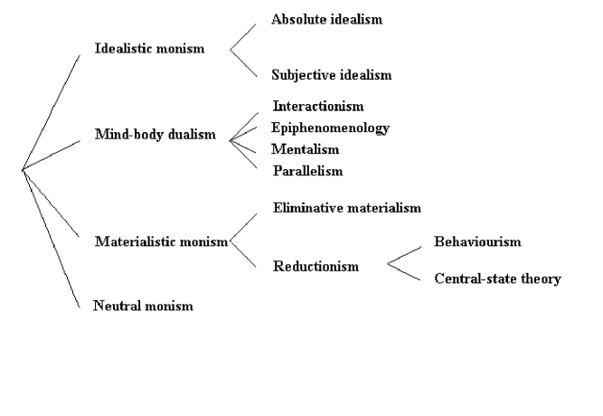
Figure III.3.1: Some philosophies of the mind

Idealism

Russell uses the term idealism for “the doctrine that whatever exists, or at any rate whatever can be known to exist, must be in some sense mental.”. It is a monistic theory as it recognises only one type of entity. It may be traced back to the Irish bishop George Berkeley [Ber10, Ber13] This belief has been very popular with philosophers over the ages.

The main argument against idealism is that elements of the physical world evolve with time in a way which is often predictable and which does not depend on whether or not I am looking at them. Even if this does not prove that these items have an independent existence, it makes it a lot simpler to assume that they do. And there is, after all, no evidence whatsoever that they do not.

(One interpretation of quantum mechanics, the many-minds interpretation [Chapter III.6] is arguably idealistic.)

Materialism

At the other extreme is materialism, another monistic theory, the doctrine that the physical universe is all that exists. It may be traced back to the early Greeks.

How does this doctrine explain sensations and emotions? In one version it is believed that these words should be eliminated altogether from the philosopher’s vocabulary, at least for the purpose of describing facts. In the other version, reductionism, sensations and emotions may be explained as complex physical phenomena. That is, the study of the mind can in principle be reduced to the study of chemistry and physics. They may either be explained as nothing more that types of behaviour (behaviourism) or as particular states of neurons in the brain (central-state theory or the identity thesis).

Materialism gains credence from recent progress in understanding the brain (eg. [Kon93, LeD94]), work which has not found any need for a mind.

Materialism is very much in vogue at the moment following the proclamation by Francis Crick and Chrostof Koch (the former of double-helix fame) in 1990 that the time is ripe for science to tackle consciousness (see [Cri94]). This has helped to inspire “an intellectual stampede” of ‘scientific research’ into consciousness [Hor94].

This doctrine, by definition, precludes consciousness from having a privileged role in quantum mechanics.

Dualism

Mind-body dualism, or psychoneural dualism, is the doctrine that the mind or consciousness exists as an entity separate to the physical universe. In this model, there is an objective physical universe and, in addition, associated with humans and perhaps some other beings is an extra-physical mind which observes (and possibly influences) the universe. This view may be traced back to Plato although it is Rene Descartes [Des42] who gave the best known formulation.

Advocates of this view may accept that the behaviour of a fellow human can be understood without assuming that they have an extra-physical mind. But they feel that their own sensations must be extra-physical. After all, one could imagine a human-body obeying the law of physics without having any sensations. The advocate of dualism believes that he or she must comprise more than ordinary matter and, for philosophical or emotional reasons, believes that other humans, and perhaps animals, must be conscious in the same way.

Do the body and mind interact? Descartes thought that they do. The mind observes the world but also influences it; for example, one makes a conscious decision to move one’s arm. This is called interactionism.

Others have suggested that the decision to move an arm is made by the physical brain and the mind can do nothing but observe. This is epiphenomenology. Still others have suggested that the mind can affect the body but is not affected by it. This is mentalism. Finally, in a view that goes back to Leibniz, it has been suggested that the mind and brain do not interact at all but work in parallel maintaining corresponding states, rather like synchronised clocks. This view is called parallelism or, more fully, psycho-physical parallelism.

Neutral monism

There is one more form of monism which warrants a mention, neutral monism. In this doctrine there is only one type of entity which is neither purely physical nor purely mental. This doctrine was first proposed by Benedict de Spinoza [Spi77] and various other forms have been proposed since.

Science and philosophy

Scientists may, for the most part, ignore the multitude of theories of the mind. Their job is to model the physical world and they have been able to do so, up to know, without assuming any kind of mind whatsoever. Almost without exception, scientists believe, perhaps implicitly, that their success in modelling the physical world without reference to the mind, vindicates the idea that the physical world exists in its own right. In terms of philosophical models, this means that scientists tend to be materialists or dualists.

Many scientists believe that it is possible to model the physical universe completely without reference to the mind, ie. they believe that the mind does not affect the physical world and so reject any form of interactionism or mentalism.

In fact, many scientists are materialists, ie. they reject the existence of anything outside the physical universe. (In a cynical assessment of this, Wigner [Wig67] writes “The reason is probably that it as emotional necessity to exalt the problem to which one wants to devote a lifetime.”.)

In this context, it is easy to see why the present interpretation, which stipulated a form of interactionism, is often rejected out of hand.

Criticism

One important difficulty with this interpretation is that it assumes a very specific model of the mind, a dualistic interactionist model. However, even if this model is accepted, the interpretation is problematic.

Firstly, it is often criticised for giving predictions which are not clear-cut in that they depend on which animals are conscious and on the precise nature of the measurements performed by the mind. However, this criticism is unscathing as these open questions could, in principle, be settled by experiment. It is true that even with the arsenal of modern invasive and non-invasive techniques for observing the brain, the above experiments will not be feasible for the foreseeable future. But the interpretation is a good theory in that it has testable consequences and in that it prescribes a scientific programme for filling in the unspecified parameters.

A more serious criticism is hinted at by Bohm and Hiley [BH93, §2.4]. They write that “it is difficult to believe that the evolution of the universe before the appearance of human beings depended fundamentally on the human mind”. This criticism can be expanded as follows. Assuming that the only minds belong to humans and to certain animals, the universe in this interpretation would initially undergo no wave function collapse. If that were true, the universe’s wave function would become a linear superposition of many different possibilities and human beings or animals would not come into existence at any well-defined moment. It is therefore difficult to see at what point minds could start to observe the universe.

Bohm and Hiley write “Of course one could avoid this difficulty by assuming a universal mind. But if we know little about the human mind, we know a great deal less about a universal mind. Such an assumption replaces one mystery by an even greater one.”. Indeed, if the interpretation were correct and if there were minds observing points outside human and animal brains, we would not know were to start looking for the quantum effects they must be causing!

Variations

Some have suggested that the mind not only observers the universe causing a random collapse of the wave function but that rather it chooses between different quantum alternatives [Mar67, Mar68, Wal74, WH77, Mar84] This is seen as a way of attributing free will to the mind.

In the normal version of the interpretation, it was shown that the effects of the mind could be detected by sensitively analysing the brain. But if the mind can actually choose between alternatives, its effects could be detected outside the body. (Unless the mind is in some way forced to obey Copenhagen statistics in the long run.)

For example, if Schrödinger had many cats each sharing a box with a bomb in the normal way then when he observed the cats his brain would be in a linear superposition of seeing them alive and seeing them dead and his mind could choose to make them all alive thereby causing a blatant deviation from the predictions of quantum theory. (There have been claims that the mind can be seen to exert just such an influence on macroscopic objects in the lab [For69]!)

Conclusion

The interpretation ties down the Copenhagen model by saying that the only true measuring apparatus are non-physical minds. Unlike the previous two interpretations, it is ontological and is not inherently ambiguous.

For those who accept the philosophical arguments for dualism and are not scared of a little interactionism, this interpretation seems attractive. Even so, it does not allow sensible discussion of the big-bang and evolution.

Scientists must hope for a different interpretation of quantum mechanics.

Bibliography

This idea is advocated by [Neu55] (especially §VI.1), [LB39] (especially §11), [Wig67] and criticised all over the place.

An excellent concise overview of the various philosophical approaches to the mind-body question may be found in [Sha76]. A well known known philosophical discussion of the relevant issues is [Rus12]. A classification of the various views may be found in [Bun77].

Chapter III.4 Hidden variables

I$\ldots$ believe$\ldots$ that the flight into statistics is to be regarded only as a temporary expedient that bypasses the fundamentals.

Albert Einstein, [Ein38]

Introduction

The statistical results of quantum mechanics seem at first sight reminiscent of the non-deterministic results of statistical mechanics. The latter result from underlying laws which are deterministic. Could the same be true of quantum mechanics? Could quantum mechanics be incomplete?

The hidden variables programme suggests that in the complete theory, every quantum system is always in a state in which every observable has a definite value. The predictions of quantum mechanics reflect the fact that there is no mechanism for completely observing or controlling every aspect of a system’s state. Ie. there is no way to prepare an ensemble of systems in which every system has the same position and the same momentum even though such an ensemble may exist. In fact, the maximal knowledge we can ever obtain may be summed up by a vector in Hilbert space. It is precisely for this reason that the specification of the state beyond the state vector is called hidden.

There exist no hidden variables theories at least in the broad sense described above. Work on hidden variables has in fact often concentrated on proving that such theories cannot exist. This chapter therefore does not describe a theory. Instead, it outlines what would constitute a hidden variables theory and discusses the proofs that no such theories exist.

Formulation

The following might be given as the definition of a completion of a quantum mechanical system.

Definition III.4.1 (Completion)

Let a quantum mechanical system have states given by the Hilbert space ${\cal H}$ and have Hamiltonian $\hat{H}$. A completion of this system is a tuple $(\Omega,U,V,\mu)$ where

• $\Omega$ is a set (the hidden states)

• for every state $s\!\in\!\Omega$ and densely define self-adjoint operator $\hat{Q}$, $V(s,\hat{Q})$ is a value in the spectrum of $\hat{Q}$ (so in each state each physical quantity has a definite value — this is often expressed by saying that the states in $\Omega$ are ‘dispersion free’)

• for every $t\!>\!0$, $U_{t}:\Omega\rightarrow\Omega$ is a map which has a measurable inverse (giving the time evolution over a time interval of length $t$) where the $\sigma$-field of subsets of $\Omega$ generated by the subsets

  $$\left\{\rule{0.0pt}{12.91664pt}\right.s\!\in\!\Omega\>|\>V(s,\hat{Q})\!\in\!(a_{1},a_{2}]\left.\rule{0.0pt}{12.91664pt}\right\}$$

  are called measurable

• for every $|\psi\rangle\!\in\!{\cal H}$, $\mu_{|\psi\rangle}$ is a probability measure on $\Omega$ defined on some $\sigma$-field including the sets called measurable above (giving the ratios of systems with different states in $\Omega$ in an ensemble described by $|\psi\rangle$)

such that

• the values of observables are consistent with relationships between the observables

  $$V(s,f(\hat{Q}))=f(V(s,\hat{Q}))\quad(\forall s\!\in\!\Omega,\hat{Q},f\!:\!{\mathbb{R}}\rightarrow{\mathbb{R}}\mbox{ Borel measurable})$$

• the ensemble defined by $\mu_{|\psi\rangle}$ gives Copenhagen statistics:

  $$\mu_{|\psi\rangle}\left(\rule{0.0pt}{12.91664pt}\right.\{s\!\in\!\Omega\>|\>V(s,\hat{Q})\!\in\!B\}\left.\rule{0.0pt}{12.91664pt}\right)=\Pr\left(\rule{0.0pt}{12.91664pt}\right.Q\!\in\!B\,;\,|\psi\rangle\,\left.\rule{0.0pt}{12.91664pt}\right)\quad(\forall Q,\psi,B\mbox{ Borel})$$

• the composure of the ensemble associated with a quantum system does not change with time (although its constituent systems do, of course, evolve with time)

  $$\mu_{e^{-i\hat{H}t/\hbar}|\psi\rangle}(U_{t}(K))=\mu_{|\psi\rangle}(K)\quad(\forall t\!>\!0,\psi,K\subseteq\Omega\mbox{ measurable})$$

• it is consistent to assume that the wave function collapses

  $$\frac{\mu_{|\psi\rangle}\left(\rule{0.0pt}{12.91664pt}\right.K\cap\{s\!\in\!\Omega\>|\>V(s,\hat{Q})\!\in\!B\}\left.\rule{0.0pt}{12.91664pt}\right)}{\mu_{|\psi\rangle}\left(\rule{0.0pt}{12.91664pt}\right.\{s\!\in\!\Omega\>|\>V(s,\hat{Q})\!\in\!B\}\left.\rule{0.0pt}{12.91664pt}\right)}=\mu_{\hat{P}|\psi\rangle}(K)\quad(\forall K\subseteq\Omega,Q,\psi,B\mbox{ Borel})$$

  where $\hat{P}$ projects onto eigenvectors of $\hat{Q}$ with eigenvalues in $B$ (this represents the case when $Q$ is measured in an ensemble in state $|\psi\rangle$ and the systems with result in $B$ are selected).

A completion in the above sense would provide a deterministic theory in which all the predictions of quantum mechanics hold.

In fact, the programme of completing quantum mechanics runs into difficulties long before the details of ensembles of dispersion free state are considered. The debate about hidden variables has centred on the feasibility of finding any dispersion free states $s$ with sensible associated values $V(s,\hat{P})$. In order to concentrate on this problem, a dispersion free state may be viewed more abstractly as a map from operators to ${\mathbb{R}}$.

Definition III.4.2 (Dispersion free state)

A dispersion free state is a map $V$ from self-adjoint operators to ${\mathbb{R}}$ which maps every observable $P$ to a value in the spectrum of $\hat{P}$ such that

• the values of observables are consistent with relationships between observables

  $$V(f(\hat{Q}))=f(V(\hat{Q}))\quad(\forall\hat{Q},f\!:\!{\mathbb{R}}\rightarrow{\mathbb{R}})\mbox{ .}$$

The trouble is that no such states exist. This is shown under Criticism.

Measurement

It is not immediately apparent whether a hidden variables theory would facilitate the modelling of measurement within the theory. After all, in the above formulation the world is still split into system and observer. Whether the observed can be brought within the system more successfully that in ordinary quantum mechanics is an open question.

There is, however, room for optimism on this point. In quantum mechanics one could not describe the whole universe within the formalism because doing so led to the strange result that nothing ever has a definite state. On the other hand with hidden variables, the hidden variables may provide this definiteness. Just such an approach is taken in Bohm’s interpretation, Chapter III.7.

Determinism

A hidden variables theory is completely deterministic. It is of course this which motivates the programme.

Locality

One of the original motivations of hidden variables theories was to eliminate nonlocality from quantum theory. If the spin in an EPR experiment is determined by hidden variables, each particle will have a definite $z$-component of spin all along and measuring the spin of one merely reveals the spin of the other without influencing it.

However, a famous paper by Bell established that nonlocality is implied not only by the Hilbert space formalism but by the statistical predictions of quantum mechanics. Any hidden variables theory which reproduces the statistical predictions of quantum mechanics would necessarily be nonlocal. A far simpler version of Bell’s argument is reproduced here from [Mer90c, Mer90a, Mer90b].

Proof of nonlocality

Consider three particles numbered $1$, $2$ and $3$ of spin ${\textstyle\frac{1}{2}}$. Write eg. ${1x}$ for the $x$ component of spin of particle $1$ and $\hat{\sigma}_{1x}$ for the associated operator. These satisfy the commutation relations

$$[\hat{\sigma}_{nx},\hat{\sigma}_{ny}]=i\hat{\sigma}_{nz},\quad[\hat{\sigma}_{ny},\hat{\sigma}_{nz}]=i\hat{\sigma}_{nx},\quad[\hat{\sigma}_{nz},\hat{\sigma}_{nx}]=i\hat{\sigma}_{ny}$$

with other commutators vanishing.

It is an easy matter to check that the three operators $\hat{\sigma}_{1x}\hat{\sigma}_{2y}\hat{\sigma}_{3y}$, $\hat{\sigma}_{1y}\hat{\sigma}_{2x}\hat{\sigma}_{3y}$ and $\hat{\sigma}_{1y}\hat{\sigma}_{2y}\hat{\sigma}_{3x}$ commute. Suppose the particles are in a common eigenstate of these with each having value $1$.

The product of the three operators is $-\hat{\sigma}_{1x}\hat{\sigma}_{2x}\hat{\sigma}_{3x}$ and so the system will also be in an eigenstate of this operator with eigenvalue $1$.

But now assume hidden variables and locality. This means that each particular spin component has a definite value (which is revealed by the measurement) and that this value, for a particular particle, cannot depend on which component of spin is measured for a different particle. Let $m_{1x}$ represent the hidden value of $1x$, etc.

Now in this particular state it must be that $m_{1x}m_{2y}m_{3y}\!=\!1$ etc. Therefore

$$1=m_{1x}^{2}m_{2x}^{2}m_{3x}^{2}=(m_{1x}m_{2y}m_{3y})(m_{1y}m_{2x}m_{3y})(m_{1y}m_{2y}m_{3x})(m_{1x}m_{2x}m_{3x})=-1$$

giving the required contradiction.

To make the implications clear, suppose that a triplet of particles in the above state is repeatedly sent out with each particle going in a different direction. Suppose that at three distant sights sit three observers and each of them on each occasion measures some component of spin. They later meet and compare results.

Now suppose that the observers assume that on each occasion the $m$ values are well defined, ie. the result of their experiment was predetermined and depended only on their own experimental set up, as is the case in hidden variable theories. Looking back on their data they will all agree that an invariant property of these $m$ values is that

$$m_{1x}m_{2y}m_{3y}=m_{1y}m_{2x}m_{3y}=m_{1y}m_{2y}m_{3x}=-m_{1x}m_{2x}m_{3x}=1$$

since each of these identities held true in every experiment which happened to test it. But the observers then find that no six integers satisfy these equations!

The result of each individual experiment cannot be predetermined. If one wants to insist that the world is deterministic, the only was is to assume that the result of the three experiments is predetermined only in terms of the experimental apparatus of all three observers. In other words, the result of one experiment depends nonlocally on the apparatus set up at the other sights.

In conclusion, from the predictions of quantum mechanics (as opposed to the formalism) it follows that if the world is deterministic it is nonlocal.

Philosophy

It is a little futile to discuss in any detail the philosophy behind a non-existent theory. Suffice to reword the discussion under Measurement and to say that although one might initially be looking for an epistemological hidden variables theory, one might expect such a theory to easily yield an underlying ontological theory.

Criticism

What is proved by impossibility proofs is lack of imagination.

A ‘suspicion’ aired by John S. Bell, [Bel82]

Consider a quantum mechanical system with states given by the Hilbert space ${\cal H}$ and with Hamiltonian $\hat{H}$.

Do there exist dispersion free states?

The proof of von Neumann

This theorem is mainly of historical interest. As will be seen, Gleason’s theorem leads to a much more general result.

Theorem III.4.3

There are no dispersion-free states with the following additional property.

• The values of (even non-commutative) operators are additive.

  $$V(\hat{P}\!+\!\hat{Q})=V(\hat{P})+V(\hat{Q})\quad(\forall s\!\in\!\Omega,\hat{P},\hat{Q})\mbox{ .}$$

$\Box\!\!\!\!$

The imposition of C.1+ is dubious. If $\hat{P}$ and $\hat{Q}$ do not commute then measuring $P$, $Q$ and $P\!+\!Q$ involves three totally different experiments. $P\!+\!Q$ is the sum of $P$ and $Q$ only in the formal mathematical sense that the operator associated with $P\!+\!Q$ is $\hat{P}\!+\!\hat{Q}$.

Therefore, although it happens to be a fact that

$$E(\hat{P}+\hat{Q})=E(\hat{P})+E(\hat{Q})$$

for the expectation values in quantum mechanics, there is no reason to expect this to hold for arbitrary states in some completion of quantum mechanics (although it must hold for quantum ensembles). The postulate described by von Neumann as ‘very general and plausible’ is ‘absurd’ [Bel82]!

This point may be emphasised by constructing a time-independent completion for a two-dimensional system, eg. for a particle of spin ${\textstyle\frac{1}{2}}$ ([Bel66, §2], [KS67, §VI]) in which, of course, C.1+ is violated.

The proof of Jauch and Piron

The same conclusion is proved by Jauch and Piron [JP63], starting from the following weaker premises.

• If $\hat{P}_{V}$ and $\hat{P}_{W}$ are projections and  $V(\hat{P}_{V})=V(\hat{P}_{W})=1$  then  $V(\hat{P}_{V\cap W})\!=\!1$.

It is easy to see that this follows from C.1+.

Bell [Bel66] however argues that the property in C.1+ is once again peculiar to quantum mechanics and that there is no reason to expect this to hold in some new theory. It is true that every element in an ensemble with state in $V\cap W$ will have to have this property. But there may be other hidden states which do not appear in such ensembles and which violate this property.

Implications of Gleason’s theorem

Theorem III.4.4

Let ${\cal H}$ be a separable Hilbert space of dimension more than two. Then there are no dispersion free states for ${\cal H}$.

Proof   Suppose $V$ were a dispersion free state. Define a map $\mu$ from the lattice of closed linear subspaces of ${\cal H}$ to ${\mathbb{R}}^{+}$ by letting $\mu(U)\!=\!V(\hat{P}_{U})$ (in fact $\mu$ must take the values $0$ or $1$). It will be shown that this map satisfies the conditions of Gleason’s theorem (Theorem II.1.7).

Let $U_{1},\ldots,U_{n}$ be orthogonal linear subspaces of ${\cal H}$. Let

$$\hat{A}=\sum_{i=1}^{n}\hat{P}_{U_{i}}=\hat{P}_{\sum U_{i}}\mbox{ .}$$

Now $\hat{A}$ and the $\hat{P}_{U_{i}}$ all commute so, by a well-known theorem, each is a function of some common operator $\hat{Q}$. C.1’ will therefore imply that

$$V(\hat{A})=V(\hat{P}_{\sum U_{i}})=\sum_{i}V(\hat{P}_{U_{i}})\mbox{ .}$$

Thus, $\mu(\sum U_{i})\!=\!\sum\mu(U_{i})$.

Then Gleason’s theorem implies that there is some density matrix such that

$$\mu(U)=\operatorname{Tr}(\hat{\rho}\hat{P}_{U})$$

for all $U$. This in turn implies that the state is not dispersion free after all because there will always be some assertions which are neither true or false (eg. either a projector tying down position or one tying down momentum). $\Box\!\!\!\!$

Is this the final nail in the coffin of hidden variables? Bell [Bel66] argues that even the condition C.1’ (Definition III.4.2) is unreasonable and that hidden variables which do not have property C.1’ are therefore feasible. He writes as follows.

The result of an observation may reasonably depend not only on the state of the system (including hidden variables) but also on the complete disposition of the apparatus.

As an example, suppose $\hat{A}=f(\hat{P})$ and $\hat{A}=g(\hat{Q})$. Then it so happens that in quantum mechanics one can measure $A$ by measuring $P$ and applying $f$ or by measuring $Q$ and applying $g$. In each case one is obtaining different side information; the first type of measurement reveals the value of any $\hat{B}=f^{\prime}(\hat{P})$ while the second reveals the value of any $\hat{B}=g^{\prime}(\hat{Q})$. However, since in quantum mechanics the statistical predictions for $A$ are the same in both kind of measurement, one becomes accustomed to thinking of $A$ as a physical observable and of the two experiments as different ways of measuring $A$.

But perhaps deep down there is no physical observable called $A$ and the two experiments are revealing different properties which happen to have the same statistical distributions in the ensembles allowed by quantum theory!

Thus, the whole definition of completions and dispersion free states has been coloured by some deep rooted but unfounded assumptions about what constitutes a physical observable.

So what Gleason’s theorem tells us is that in any hidden variables theory, some quantities which appeared as coherent physical observables in quantum theory will manifest themselves as a group of distinct observables, which correspond to different experimental set ups. Such observables are called context dependent observables although this slightly obscures the point that they are not really observables. As Bell [Bel82] points out, all of this is in accord with Bohr’s philosophy that the properties of a system are inextricably tied up with the set-up of the experiment.

So it turns out that the proofs against hidden variables are disappointing. They only tell us that some quantities which seem like observables in quantum mechanics will turn out to depend on the experimental set up in a hidden variables theory. And this is not new! Bell’s theorem has already established that some results will have to depend on the experimental set up, in fact, on the experimental set up at remote sights!

Bibliography

Von Neumann’s proof is contained in [Neu55, §IV.1–2]. It is criticised in eg. [Her35, pp.99–104], [Bel66, Bel71].

The implications of Gleason’s theorem were pointed out by Jauch. The relevant corollary of Gleason’s theorem is established using elementary arguments in [Bel66]. Kochen and Specker [KS67] proved the same conclusion without starting from Gleason’s theorem. A simpler proof, for the case of two particles of spin ${\textstyle\frac{1}{2}}$ was given by Peres [Per90]. A proof for more than two particles is given in [GHSZ90]. These proofs are summarised concisely in [Mer90b].

A concise account of the proofs of von Neumann, Jauch and Piron and of the consequences of Gleason’s theorem is given in [Bel66]. A more general survey is [Bel73].

Bell’s theorem is presented in [Bel64] and again, in a slightly more general form, in [Bel71]. The theorem establishes that the statistical correlations in a certain experiment on two particles of spin one half are inconsistent with hidden variables and locality. The relevant predictions of quantum mechanics have been checked experimentally [AGR81, ADR82]. The same result may be established by considering angular momentum [Mer80].

In an alternative experimental arrangement with three particles of spin one half, there are perfect correlations which are inconsistent with hidden variables and locality [GHZ89, GHSZ90]. The proof presented above is a simplified version of this due to Mermin [Mer90c, Mer90a, Mer90b]. The implications of these results are discussed carefully in [Sta93]. The same result may be achieved considering two particles [Har92] or one particle [Cza94].

Einstein was the best know advocate of hidden variables and a nice book on his views is [Fin86].

Chapter III.5 Many-worlds interpretation

Every quantum transition taking place on every star, in every galaxy, in every remote corner of the universe is splitting our local world on earth into myriads of copies of itself.

B. S. DeWitt, [DeW71]

Introduction

At the heart of the measurement problem is the contrast between the coherent state (III.1.2):

$$(|\mbox{``up''}\rangle|\uparrow\rangle+|\mbox{``down''}\rangle|\downarrow\rangle)/\sqrt{2}\mbox{ .}$$

predicted by Schrödinger’s equation, on the one hand, and the two possible outcomes (III.1.1):

$$|\mbox{``up''}\rangle|\uparrow\rangle\mbox{ \ or \ }|\mbox{``down''}\rangle|\downarrow\rangle$$

predicted by the wave function collapse, on the other.

The many-worlds interpretation suggests that these are one and the same!

If it were possible to imagine that the two summands $|\mbox{``up''}\rangle|\uparrow\rangle$ and $|\mbox{``down''}\rangle|\downarrow\rangle$ represents equally real but separate realities then the wave function collapse would actually follow from the Schrödinger equation!

In the many-worlds interpretation, this is achieved by the bold suggestion that the summands in the coherent state represent separate worlds, existing in parallel and equally real, one in state $|\mbox{``up''}\rangle|\uparrow\rangle$ and the other in state $|\mbox{``down''}\rangle|\downarrow\rangle$.

The idea of decomposing the state into orthogonal summands to show that the unitary mechanics and wave function collapse are one and the same is highly seductive. Here, an extreme view will be taken: this observation is entirely irrelevant to the interpretation of quantum mechanics.

Why? The measurement problem arises because in studying our world it is found that both the Schrödinger equation and wave function collapse are needed. The challenge is therefore to find a way to understand both the Schrödinger equation and the wave function collapse within our world. There is no virtue in finding a way to apply the Schrödinger equation elsewhere, ie. in some collection of worlds.

The many-worlds interpretation has always been presented in a vague way along with exaggerated claims (such as “The mathematical formalism of the quantum theory is capable of yielding its own interpretation” [DeW71]) and overlooked technical problems. Nonetheless, it has received broad attention and is therefore considered here.

Formulation

Rules

The universe may be associated with a separable Hilbert space ${\cal H}$; a densely defined self-adjoint operator $\hat{H}$ on ${\cal H}$ called the Hamiltonian; and an element $|\psi\rangle\!\in\!{\cal H}$ called the initial state, in such a way that the following hold.

• At any time, the universe comprises a countable number of worlds each of which has a space-time like our own world and each of which may be described by a state in ${\cal H}$. The worlds have a branching structure, ie. sometimes one world splits into countably many worlds.

• Parallel worlds at one time have orthogonal states.

• The total state of any subset of the branches evolves according to Schrödinger’s equation with Hamiltonian $\hat{H}$.

• If one assigns a measure $\langle\psi|\psi\rangle$ to a world in state $|\psi\rangle$ (the previous rule implies that this measure is conserved across a split) then one should only expect to reproduce the predictions of quantum mechanics in almost all worlds (with respect to this measure).

• The way in which vectors in ${\cal H}$ describe the world is understood using orthodox quantum mechanics, ie. self-adjoint operators and the like.

The ontology is sketched in Figure III.5.1.

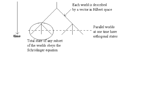
Figure III.5.1: The many-worlds ontology

Discussion

At any one time the states of parallel worlds are orthogonal so these states may be normalised and extended (perhaps in many ways) to a complete orthonormal set of vectors. Such a set is called a preferred basis.

Conversely, given that $|\psi_{1}\rangle,|\psi_{2}\rangle,\ldots$ is a preferred basis at some time, the global state may be decomposed into the form $\sum_{i}a_{i}|\psi_{i}\rangle$ giving the states of the different worlds at that time: $a_{1}|\psi_{1}\rangle,a_{2}|\psi_{2}\rangle,\ldots$ (ignoring zeroes).

The interpretation is still incomplete in that it does not give details of the branching structure or of the preferred basis and its time evolution.

It is necessary to check that the rules can be satisfied. Suppose that an arbitrary branching structure is fixed. At any time when no splitting occurs, the state of each world must evolve according to the Schrödinger equation. (This means that the elements of the ‘preferred basis’ are also evolving according to the Schrödinger equation. One cannot have a fixed preferred basis.)

What happens at a split? Of course, the total state must not change discontinuously. What happens is that a world in state $|\psi\rangle$ splits into worlds with orthogonal states $|\phi_{1}\rangle$, $|\phi_{2}\rangle$,$\ldots$, where $|\psi\rangle=\sum_{i}|\phi_{i}\rangle$. (This corresponds to a discontinuous change in the preferred basis.)

This is sufficient to ensure that all the rules are satisfied.

Achievements

What has been achieved? Consider one branch. At times the state of that branch evolves in accordance with the Schrödinger equation. At other times (at the splits) it undergoes a wave function collapse.

This, of course, is a possible way to solve the measurement problem. The world obeys the Schrödinger equation except that the wave function sometimes collapses ensuring that things have some sort of definite state. Of course, the big question is when and how this collapse occurs and the many-worlds interpretation has left this completely open.

So what has been gained by assuming many-worlds? Merely that it might be possible for the entire collection of worlds to be described by Schrödinger’s equation. This, as already argued, is no gain at all.

Measurement

There is one thing that works in the many-worlds interpretation, namely that the Copenhagen statistics for a measurement are reproduced. This does assume that things have been sorted out so that the preferred basis at the end of the measurement is precisely a basis consisting of the eigenstates of the system and apparatus (tensor producted with some states for the rest of the world). (Of course, the central difficulty with this type of interpretation is how to sort things out so that this always holds. This in turn requires a rigorous definition of a measurement.)

Consider a system with normalised eigenstates $|\chi_{1}\rangle,|\chi_{2}\rangle,\dots$ coupled with an observer in initial normalised state $|\phi\rangle$ in such a way that over a specified time the initial state $|\phi\rangle\otimes|\chi_{i}\rangle$ evolves into the normalised state $|\phi_{i}\rangle\otimes|\chi_{i}\rangle$ in which the observer has completed the measurement and has a record of the result.

Let $|R\rangle$ be the state of the rest of the world and assume that $|R\rangle\otimes|\phi_{i}\rangle\otimes|\chi_{i}\rangle$ is a part of a preferred basis at this time.

What is the result of performing a measurement on the normalised state $\sum_{i}a_{i}|\chi_{i}\rangle$ ? Of course, the state $|R\rangle\otimes|\phi\rangle\otimes\sum_{i}a_{i}|\chi_{i}\rangle$ evolves to the state $|R\rangle\otimes\sum_{i}a_{i}(|\phi_{i}\rangle\otimes|\chi_{i}\rangle)$ in which there are a number of worlds in each of which a specific value has been measured.

In the world where the observer measured value $i$ (that is where the observer is in state $|\phi_{i}\rangle$), the state of the system is $|\chi_{i}\rangle$ after the measurement, ie. each observer observes the wave function collapse predicted in the Copenhagen interpretation.

To check that the Copenhagen statistics are observed, it is necessary to consider the same experiment on an ensemble.

Consider an ensemble of $n$ copies of the system and a team of $n$ observers with states

$$|\boldsymbol{\phi}\rangle=|\phi\rangle\cdots|\phi\rangle\quad\quad|\boldsymbol{\phi}_{i_{1},\dots,i_{n}}\rangle=|\phi_{i_{1}}\rangle\cdots|\phi_{i_{n}}\rangle\mbox{ .}$$

Then the initial state

$$|R\rangle\otimes|\boldsymbol{\phi}\rangle\otimes\left[\left(\sum_{i}a_{i}|\chi_{i}\rangle\right)\otimes\cdots\otimes\left(\sum_{i}a_{i}|\chi_{i}\rangle\right)\right]$$

evolves into the state

$$|R\rangle\otimes\sum_{i_{1},\dots,i_{n}}a_{i_{1}}\cdots a_{i_{n}}|\phi_{i_{1},\dots,i_{n}}\rangle\otimes|\chi_{i_{1}}\rangle\otimes\cdots\otimes|\chi_{i_{n}}\rangle\mbox{ .}$$

It must now be assumed that each of these summands is in a preferred basis.

The measure of the observer who observes the sequence $i_{1},\dots,i_{n}$ is $|a_{1}|^{2}\cdots|a_{n}|^{2}$. It follows that as $n\rightarrow\infty$, the measure of observers who observe the proportion of results $i$ to be within $\epsilon$ of $|a_{i}|^{2}$ tends to one. In the limit, almost all observers obtain the probabilities predicted by the Copenhagen interpretation.

Note that it is also easy to check that almost all observers will obtain the results predicted by Schrödinger’s equation if they wait before performing the measurement.

Determinism

The interpretation is deterministic. This does not, however, allow definite predictions to be made because a typical prediction will be wrong in most futures.

Locality

In the many-world interpretation an experiment performed at one point in the universe causes a split at all points in the universe. In this sense, the interpretation cannot be considered local.

Philosophy

The interpretation presents a bizarre realistic ontology.

Criticism

The central difficulty with the many-worlds interpretation is that it is formulated so vaguely as to hardly warrant the title interpretation. With no indication of how to sort out the preferred basis and branching structure, the interpretation has achieved nothing.

The other disturbing feature of this interpretation is the ontological extravagance of an infinity of parallel worlds. (These are intended to recover the Schrödinger equation.)

Another criticism of the interpretation which is sometimes raised (eg. [Alb92, p.115]) is what sense can be made, in the interpretation, of the statement that an event will happen with probability $p$? However, sense can be made of this by saying that (in almost all futures) if the experiment is repeated many times then the given result will occur with frequency $p$.

Variations

Some people try to avoid the extravagance of many-worlds by talking about one world with many stories (eg. [Loc89]). However, it is not at all clear what this really means.

It is possible to avoid the extra worlds by assuming that only one survives. Explicitly, one may assume that whenever the world branches, only one world is retained, it being chosen probabilistically with probability proportional to the branch’s measure in the ordinary many-worlds interpretation. This has been called the one-world version of the many-worlds interpretation [Hea84]. It is the version which Bell considered most defensible. It is, of course, not a theory with many-worlds although there are still many possible future worlds of which one will be realised.

It seems that in the many-worlds interpretation one can choose between a deterministic universe with many worlds and a stochasticly governed universe with one world.

Conclusion

The many-worlds interpretation makes no progress in helping us to understand the wave function collapse. It introduces extra worlds to allow Schrödinger’s equation to be recovered but this is pointless.

Bibliography

The many-worlds interpretation was introduced as the “relative state” formulation of quantum mechanics by Hugh Everett III in his PhD dissertation [Eve57a]. A fuller account is [Eve57b]. The book [DG73] reproduced these and some other papers explaining the many-worlds interpretation.

Everett did not explicitly say that the different summands represented different worlds but only that at each observation “the observer state ‘branches’ into a number of different states” and that “all branches exist simultaneously”. De Witt [DeW70, DeW71] and others added the idea of many-worlds (mistakenly attributing this idea to Everett).

A thorough discussion of the development of the interpretation is included in [BD87]. Other discussions of many-worlds include [CvV69, Zeh71, Pri81, Hea84, Ger84, Ste84, AL89], [d’E76, Ch.20],[BH93, Ch.13]. A typical philosophical reaction to the interpretation is [Gib87].

The interpretation is criticised in several papers of Bell (eg. [Bel76, Bel81, Bel86]) for the vagueness regarding the preferred basis problem, for simplistically treating instruments as single particles, and for extravagance. Bell and others [Bal73] also criticised the exaggerated claims such as quantum mechanics ‘yields its own interpretation’. The interpretation is also criticised in [Bar92].

[Alb90] points out the surprising result that one observer can prove to another that the latter exists in two universes.

Astoundingly, presumably for lack of choice, the interpretation is accepted by many cosmologists. Some have gone so far as to consider travelling to parallel universes (eg. [DL94] for a non-technical discussion).

Chapter III.6 Many-minds interpretation

We have little doubt that the MMV (many-minds view)
will invoke in most readers an “incredulous stare”.

David Albert and BarryLoewer [AL89]

Introduction

The many-minds interpretation accepts Everett’s idea that all results of an experiment are equally real but shies away from the idea that this involves making an infinite number of copies of the universe. Instead, different minds perceive the different results.

Formulation

Rules

The universe may be associated with a separable Hilbert space ${\cal H}$; a densely defined self-adjoint operator $\hat{H}$ on ${\cal H}$ called the Hamiltonian; and an element $|\psi\rangle\!\in\!{\cal H}$ called the initial state, in such a way that the following hold.

• The state of the universe may be represented by a vector in Hilbert space which evolves according to Schrödinger’s equation with Hamiltonian $\hat{H}$.

• Each conscious brain in the universe is associated with many non-physical minds. There is a specific set of normalised orthogonal states of a brain written $|B_{1}\rangle,|B_{2}\rangle,\ldots$ for each of which the attached mind is in a given state, ie. these brain states correspond to particular sensations. (States of the mind may therefore be labelled $B_{1},B_{2},\ldots$.)

• Suppose the universe is in state $\sum|B_{i}\rangle|R_{i}\rangle$ where the $|R_{i}\rangle$ are normalised states of the rest of the world. Suppose that $|B_{i}\rangle|R_{i}\rangle$ evolves over time to the state $\sum_{j}b_{j}|B_{j}\rangle|R_{j}^{\prime}\rangle$ with the $|R_{j}^{\prime}\rangle$ normalised. Then the probability that any one mind initially in state $B_{i}$ ends up in state $B_{j}$ is $|b_{j}|^{2}$.

There is an immediate difficulty with this formulation, similar to the vagueness regarding the branching structure in the many-worlds interpretation.

In order to decide the probability for a particular mind to be in a particular state $B_{i}$ at time $t$, one may look at its state at some earlier time and the above rule will give the probability. But for each earlier time there will be such a probability! In general these probabilities will all be different.

Of course, it is always possible that with a large enough set of minds the allocation could be done very cleverly so that all the rules of probabilities are satisfied. It is just that nobody has ever been clever enough to propose such a scheme.

Measurement

In this interpretation, a measurement occurs when a conscious brain becomes aware of the result. For example, let $\hat{A}$ be an observable on some system with spectrum $|A_{1}\rangle,|A_{2}\rangle,\ldots$ and let $|``A_{i}\mbox{''}\rangle$ (equal to some $|B_{j}\rangle$) represent the state of a brain which has noted the value of $A$ to be $i$.

A measurement consists of a chain of interactions under which any state $|?\rangle|A_{i}\rangle$ evolves into the state $|``A_{i}\mbox{''}\rangle|A_{i}\rangle$.

To see that the orthodox statistics are reproduced, let a system be in state $|A_{i}\rangle$. Someone measures the state leading to a state $|``A_{i}\mbox{''}\rangle|A_{i}\rangle$. Now suppose the two systems evolve independently for a time into state $|?\rangle(\sum_{i}a_{i}|A_{i}\rangle)$. Another measurement changes this into state $\sum_{i}a_{i}|``A_{i}\mbox{''}\rangle|A_{i}\rangle$. Of the minds which originally perceived $``A_{i}\mbox{''}$ the rules dictate that a proportion $|a_{j}|^{2}$ now perceive $``A_{j}\mbox{''}$ in accordance with the orthodox statistics.

Determinism

The state of the universe evolves deterministically but the state of a given mind evolves probabilistically.

Locality

The inventors of the interpretation claim that it is local. In the EPR situation, when each observer measures the $z$-component of spin, half of their minds perceive it to be up and the other half of their minds perceive it to be down. It makes no difference in what order the experiments are performed. (Even so, if both observers write down the result then all minds will perceive the results to be anti-correlated.)

More generally, it is easy to check that the probabilistic evolution of the state of a mind does not depend on what happens in a part of the universe which is isolated from the associated brain or on what happens to a mind attached to a distant brain.

Nevertheless, there is a sense in which the interpretation is not local. Considering again the EPR situation, when a particular mind becomes committed to seeing the local particle’s $z$-component of spin as being up or down, it is also being committed to seeing the distant particle’s $z$ component as being, respectively, down or up. So, as in orthodox quantum mechanics, the local experiment causes the distant particle to take on a definite $z$-component of spin, at least as far as the local mind is concerned (even though the distant minds will be unaffected).

This ambiguity in the understanding of locality is due to the fact that the interpretation is mainly concerned with describing minds (ie. it is idealistic, see Philosophy below). As such, it is not terribly clear that the concept of locality is even relevant.

Philosophy

The interpretation is most easily understood as being idealistic. In other words, it assumes that no universe exists independently of minds and that Schrödinger’s equation may be used to predict the time evolution of minds. There may be many conscious entities each associated with infinitely many minds and their sensations are governed by a single equation so are correlated.

Criticism

It is not clear that the probability rule can be satisfied. If it can, this interpretation suffers from the same difficulty as the interpretation in which the mind causes collapse; it cannot explain the evolution of the universe prior to the appearance of (animals and) man.

Variations

The interpretation was originally formulated in terms of sets of minds so that to any one mind attached to one person’s brain their corresponded a particular mind attached to another person’s brain [AL89]. The idea was that, for example, in an EPR type situation it is this pair of minds which would be anti-correlated in their perceptions. If they ever met they could confirm this. But since minds cannot meet, this idea seems a bit pointless and indeed it was dropped [Alb92].

Conclusion

The fact that this interpretation is extremely bizarre would be more palletable if the technical stuff actually worked.

Bibliography

The interpretation is presented in [AL88, Alb88, AL89] and [Alb92, esp. pp.130–133].

Chapter III.7 Bohm’s interpretation

The God of the BB (Bohm-Bell) view doesn’t play dice
but he has a malicious sense of humor.

David Albert and Barry Loewer, [AL89]

Introduction

Bohm’s interpretation of quantum mechanics came about not so much as an attempt to solve the measurement problem but more as an attempt to explain the wave-particle duality. In quantum mechanics electrons, for example, display the interference properties of waves while, at the same time, coming in discrete multiples of some basic mass like particles.

In 1927 de Broglie [Bro27] suggested that the duality could be resolved by saying that an electron was a wave and a particle, ie. the wave function represents a physical field and in it moves a particle with well defined position and momentum. This theory was retracted in 1930 [Bro30].

The idea was taken up (independently) by Bohm in 1952 [Boh52]. Here it was cast as a hidden variables theory in which the position of the particle is the hidden variable.

Later Bohm stopped using the term ‘hidden variables’ and emphasised the fact that his interpretation promotes quantum mechanics from epistemology to ontology.

Here, the interpretation is first presented as a hidden variables theory. Its application to closed systems is then discussed.

Formulation

As a hidden variables theory

Bohm’s interpretation gets around the impossibility proofs with the following bold conjecture: the only true observable is position.

The interpretation may be formulated for a spinless system with $n$ generalised coordinates as follows.

Rules

The system may be associated with a self-adjoint Hamiltonian $\hat{H}$ densely defined on $L^{2}({\mathbb{R}}^{n})$, with a wave function $\psi(t,q_{1},\ldots,q_{n})$ (which may be seen as an objective physical field) and with $n$ sharply defined coordinates following continuous paths $r_{1}(t),\ldots,r_{n}(t)$, in such a way that the following hold.

• The wave function evolves according to Schrödinger’s equation with Hamiltonian $\hat{H}$.

• The rate of change $\dot{r}_{i}(t)$ of the $i$th coordinate at time $t$ is equal to

  $$\boxed{\dot{r}_{i}(t)=\frac{{\mathbb{j}}_{i}(t,r_{1}(t),\ldots,r_{n}(t))}{|\psi(t,r_{1}(t),\ldots,r_{n}(t))|^{2}}}$$ (III.7.1)

  where ${\mathbb{j}}$ is the ($n$-dimensional) probability density current for the wave function $\psi$.

• A measurement which tests in which of a number of (Borel) sets $B_{i}$ the $j$th coordinate lies at time $t$ will yield the set $B_{k}$ containing $r_{j}(t)$. It will also cause the wave function to collapse in such a way that $\psi(t,q_{1},\ldots,q_{n})$ will be zero for $q_{j}\not\in B_{k}$.

• In any ensemble of systems with wave function $\psi$, the number of systems with coordinates in the Borel set $B$ is proportional to $\int_{B}|\psi({\mathbb{r}})|^{2}d{\mathbb{r}}\mbox{ .}$

Discussion

The idea is that the sharp coordinates $r_{i}(t)$ are hidden variables determining the result of any measurement of a coordinate. A quantum mechanical ensemble with wave function $\psi$ really consists of systems all of which have wave function $\psi$ and in which the proportion of systems with coordinate values $r_{1},\ldots,r_{n}$ at time $t$ is proportional to $|\psi(t,r_{1},\ldots,r_{n})|^{2}$. If this is true at time $t$, the definition of the probability density current ensures that it stays true at all later times.

It is possible to check that this is a completion of quantum mechanics in the formal sense of Definition III.4.1 if “every self-adjoint operator $\hat{Q}$” is replaced in the definition by “each of the operators $\hat{q}_{1},\ldots,\hat{q}_{n}$”. The set of states $\Omega=L^{2}({\mathbb{R}}^{n})\times{\mathbb{R}}^{n}$; a typical state may be written $(\psi,{\mathbb{r}})$ (strictly one should call $\psi$ and $k\psi$ equivalent and consider equivalence classes). $Q((\psi,{\mathbb{r}}),\hat{q}_{i})$ is of course just $r_{i}$. The time evolution $U_{t}$ evolves the wave function according to Schrödinger’s equation and the coordinates according to (III.7.1).

For every Borel set $B\subseteq{\mathbb{R}}^{n}$, one may define $\mu_{\psi}(\{\phi\}\times B)=\delta_{\psi\phi}\int_{B}|\psi({\mathbb{x}})|^{2}\,d{\mathbb{x}}$.

It may be checked that C.1–C.4 hold.

For closed systems

The same formalism precisely may be applied to closed systems, in particular to the entire universe. Again, the $n$-dimensional spinless case is considered.

Rules

The closed system may be associated with a self-adjoint Hamiltonian $\hat{H}$ densely defined on $L^{2}({\mathbb{R}}^{n})$, with a wave function $\psi(t,q_{1},\ldots,q_{n})$ (which may be seen as an objective physical field) and with $n$ sharply defined coordinates following continuous paths $r_{1}(t),\ldots,r_{n}(t)$, in such a way that the following hold.

• The wave function evolves according to Schrödinger’s equation with Hamiltonian $\hat{H}$.

• The rate of change $\dot{r}_{i}(t)$ of the $i$th coordinate at time $t$ is equal to

  $$\dot{r}_{i}(t)=\frac{{\mathbb{j}}_{i}(t,r_{1}(t),\ldots,r_{n}(t))}{|\psi(t,r_{1}(t),\ldots,r_{n}(t))|^{2}}$$

  where ${\mathbb{j}}$ is the ($n$-dimensional) probability density current for the wave function $\psi$.

• Human experience results from a perception of the “hidden” coordinates (not from a perception of the wave function).

Discussion

It is now necessary to establish that the two presentations are mutually consistent. One must show that in a closed system one may treat any subsystem (which does not contain conscious entities) using the hidden variables formulation.

Suppose the subsystem comprises coordinate $1,\ldots,m$. Then the wave function of this subsystem may be obtained from the total wave function by

$$\psi_{0}(t,r_{1},\ldots,r_{m})=\int_{{\mathbb{R}}}\psi(t,r_{1},\ldots,r_{n})dr_{m+1}\cdots dr_{n}\mbox{ .}$$ (III.7.2)

The hidden coordinates of the subsystem are $r_{1}(t),\ldots,r_{m}(t)$ as in the total system.

The fact that an ensemble of such subsystems will tend to have a $|\psi|^{2}$ distribution is proved in [Val91a]. Note that once this distribution is obtained it will be maintained (this follows from the definition of ${\mathbb{j}}$).

When there is no interaction, the wave function and the coordinates will have the correct time evolution. When a measurement of position takes place, this must be modelled in the total system and it must be shown that the interaction preduces the result predetermined by the $r_{1}(t),\ldots,r_{m}(t)$ and that it causes the reduced wave function (III.7.2) to collapse. This will be shown under Measurement.

When Bohm’s interpretation is applied to the whole universe, the particle coordinates, far from being hidden, are the only things which we perceive. This important assumption is sometimes swept under the carpet in discussions of Bohm’s interpretation. But if our perceptions are determined by the wave function, the coordinates would play no role whatsoever. Note, however, that when considering a subset of the universe which includes no conscious brain, the particle coordinate are hidden.

Comparison with many-worlds interpretation

The many-worlds interpretation seeks to explain the definite position of macroscopic objects by writing the wave function as a sum of different vectors and saying that different vectors are experienced in different branches of the universe. Bohm’s interpretation achieves the same thing using the “hidden” coordinates and it is instructive to cast this in the language of many worlds.

Let $\psi(t,{\mathbb{x}}_{1},{\mathbb{x}}_{2},\ldots)$ be the wave function of the universe. At time $t$, this may be written as the sum

$$\psi(t,{\mathbb{x}}_{1},{\mathbb{x}}_{2},\ldots)=\int\psi(t,{\mathbb{r}}_{1},{\mathbb{r}}_{2},\ldots)\delta({\mathbb{x}}_{1}\!-\!{\mathbb{r}}_{1})\delta({\mathbb{x}}_{2}\!-\!{\mathbb{r}}_{2})\cdots\,d{\mathbb{r}}_{1}\,d{\mathbb{r}}_{2}\cdots\mbox{ .}$$

This may be interpreted as a continuum of universes. A typical world has wave function $\delta({\mathbb{x}}_{1}\!-\!{\mathbb{r}}_{1})\delta({\mathbb{x}}_{2}\!-\!{\mathbb{r}}_{2})\cdots$ and measure $|\psi(t,{\mathbb{r}}_{1},{\mathbb{r}}_{2},\ldots)|^{2}$. In each world every particle has a definite position.

A branch may be said to have the defining property that every particle moves continuously in that branch.

Now the “hidden” coordinates of Bohm’s interpretation clearly define a branch in this many-worlds model. These are a very special class of branches in which the laws of quantum mechanics are observed to hold.

Clearly, Bohm’s interpretation is not a many-worlds theory. In the first place, the above account uses uncountably many worlds. It has not been shown how to write the wave function in terms of the branches. And, most importantly, only a very special class of branches is picked out.

Nevertheless, it is interesting to see the relationship between these seemingly unrelated interpretations.

Spin

There has been an attempt to model spin in Bohm’s interpretation as the physical spin of the particle [BST55]. However this fails where there is more than one particle.

Instead, spin should be considered as a property of the wave function only. It is then only necessary to recast (III.7.1) in terms of the spinor wave function and this can be done in two ways (compare [Bel84] and [BH93, §10.4–10.5]).

Measurement

Of position

The aim now must be to recover the hidden variables version of the theory from the theory for closed systems. In other words, if the measured particle and measured apparatus are all modelled within the theory, one must derive the result that the measured position will correspond to the coordinates of the measured particles and that wave function will appear to collapse.

Consider a simple impulsive measurement of position in which a macroscopic pointer initially has wave function $\psi_{ini}$ and after the measurement has position $y$ corresponding to the measured position of the particle. This is only intended as an example and so the mathematically dubious Dirac delta functions will be used here.

During the measurement, an initial wave function $\delta(x-r)\psi_{ini}(y)$ corresponding to a particle in position $r$ evolves into the wave function $\delta(x-r)\delta(y-r)$ in which both the particle and pointer have position $r$. In this case the hidden coordinate of the particle must initially be $r$ and both hidden coordinates end up as $r$.

If, more generally, the particle initially has wave function

$$\psi(x)\psi_{ini}(y)=\int\psi(r)\delta(x-r)\psi_{ini}(y)\,dr$$

then, by linearity, it evolves into the wave function

$$\int\psi(r)\delta(x-r)\delta(y-r)\,dr=\psi(x)\delta(y-x)$$ (III.7.3)

in which the coordinate $x$ and $y$ are perfectly correlated.

What about the hidden coordinates? If the initial coordinate was $q$ for the particle then in the sharp case of an initial wave function $\delta(x-q)\psi_{ini}(y)$ the coordinates end up as $q$ for both the particle and pointer. Here we have a superposition of wave packets $\int\psi(r)\delta(x-r)\delta(y)\,dr$ but the wave packets never overlap (because of the $\delta(x-r)$ factor which does not change with time) so just one of them affects the hidden coordinates and therefore the coordinates vary in exactly the same way ending up as $q$ for both the position and particle.

Thus the hidden variables result is recovered. The final coordinate of the pointer, which is perceived by us, corresponds accurately to the hidden coordinate of the particle.

What about wave function collapse? In any further experiments on the particle, the perceived results will again be based entirely on the “hidden” coordinate of the pointer. This coordinate will evolve according to the probability density current of the wave function (III.7.3). But here again, the packets do not overlap and only the packet $\delta(x-q)\delta(y-q)$ will contribute to the behaviour of the pointer coordinate. This shows that for the purposes of predicting further results the wave function of the particle must be taken to be the collapsed form $\delta(x-q)$.

Of other observables

Measurements of other observables will not lead to definite answers.

Consider what happens if the above argument is repeated for momentum. An initial wave function $e^{ipx/\hbar}\psi_{ini}(y)$ evolves into $e^{ipx}e^{ipy}$. The more general wave function

$$\int\phi(k)e^{ikx}\psi_{ini}dk$$

evolves, by linearity, into

$$\int\phi(k)e^{ikx}e^{iky}dk\mbox{ .}$$ (III.7.4)

But here all the wave packets will affect the hidden coordinates, (not just the one with momentum equal to the initial momentum of the coordinate, for example). So the hidden coordinates will not predetermine the result. In fact, no definite result will emerge since the momentum of the hidden coordinates will not settle down to a fixed value.

In doing further calculations, all the wave packets in (III.7.4) will influence the hidden coordinates and no wave function collapse will be observed.

In conclusion, there is no measurement until there is a measurement of position.

Determinism

The theory is deterministic.

Locality

The theory is explicitly nonlocal. The velocity (III.7.1) of a particle depends on the multidimensional wave function at the point given by all the other particles. Therefore any change in the position of one particle instantly changes the velocity of the other particles.

It is reassuring, however, that if the wave function is separable (ie. if two systems have not interacted in the past) then the systems do not interact nonlocally. This is easily checked.

In any event, the nonlocal effect on a distant system may effect that system but will not have a perceptible effect on a $|\psi|^{2}$ ensemble of such systems since such an ensemble obeys the rules of quantum mechanics. This makes nonlocal communication rather difficult.

Even so, there is currently no proof that nonlocal communication is impossible in Bohm’s interpretation because there may be situations in which there is no $|\psi|^{2}$ ensemble. (This necessarily entails signal nonlocality [Val91b].)

Philosophy

The theory gives a realistic ontological model of the universe.

It gives a special role to position. The term positionism was coined in [AL89] for this philosophy!

The particles in the theory are influenced by the wave but do not influence it (epiphenomenalism) a position which offends some people’s sense of justice.

Criticism

Nonlocality has often been sighted as the interpretations least attractive feature. There are other difficulties too.

The privileged role of position

The interpretation gives position a unique role which it does not obviously deserve. It is true that most experiments on quantum system go through a stage of recording positions eg. in a photographic plate or bubble or spark chamber. But is this necessarily the case or is it just convenient in practice?

It is also no use having a measurement of position somewhere along the line — the final measurement must be of position. This really means that the information presented by the brain to the mind (be that a component of the brain or a separate entity) had better be presented using position. Otherwise, humans would not perceive the world in a definite state.

This important implication of Bohm’s theory has not been made clear up to know. Indeed one of the main attractions of the theory has been its apparent independence from any considerations of the mind.

The mysterious quantum potential

Consider a particle moving through space in Bohm’s interpretation with a wave function $\psi$. It may be checked that the fact that its velocity is given by (III.7.1) implies that the particle is subject to a potential

$$-\frac{\hbar^{2}}{2m}\frac{\nabla^{2}|\psi|}{|\psi|}\mbox{ .}$$

Bohm himself felt that this potential is “rather strange and arbitrary” and “has no visible source”. At that time Bohm accepted this as grounds for being dissatisfied with the interpretation.

Later, however, Bohm and Hiley [BH93, p.37] suggested that the wave function should not be seen as a potential pushing the particle around. Instead, the wave function acts like a map (they call this active information) guiding the particle which reads the wave function and then adjusts its own speed.

They write: “The fact that the particle is moving under its own energy, but being guided by the information in the quantum field, suggests that an electron or any other elementary particle has a complex and subtle inner structure (eg. perhaps even comparable to that of a radio).”

This suggestion seems strange. There are many ways to reassemble the parts of a radio and obtain something else. There is no evidence that the same may be done with an electron.

However, this problem and the awkward solution proposed by Bohm and Hiley only come about from trying to cast the interpretation in the familiar language of potentials. But here a new and fundamental theory of the universe is being proposed and there is no reason to expect it to conform to this model. Instead, the formula (III.7.1) for velocity, which seems neither strange nor arbitrary, may be taken as a new fundamental law of physics.

Variations

In one variation it is assumed that there are sub-quantum fluctuations. These ensure that every ensemble rapidly reaches a $|\psi|^{2}$ distribution [BV54, Nel66, BH89].

Bohm’s interpretation does not extend naturally to quantum field theories because such theories lack a position observable. However, versions of the interpretation do exist for the electromagnetic field [Boh52, Appendix], the Fermi field [Bel84] and for Boson fields [BH93, Ch.11].

Conclusion

Bibliography

The idea of the wave function guiding a particle was originally presented in [Bro27] for a one-body system. In this presentation it was suggested that a non-linear modification of the Schrödinger equation might give rise to a stable singularity or pulse (corresponding to Bohm’s particle) with values elsewhere agreeing with the ordinary wave function. This idea was called double solution. This was criticised at the 1927 Solvay congress particularly by Pauli [Pau28]. The most important criticism was that the theory did not explain two-particle experiments. Indeed, the double solution has never been extended to many particles.

The social reasons for the theory’s rejection are discussed in [Pin77, Cus94]. The theory was retracted [Bro30].

The theory was again and independently proposed, in great detail, by Bohm [Boh52]. Bohm encouraged de Broglie to take it up again [Bro56a, Bro56b]. Interestingly,

Einstein found the theory “too cheap” [Bor71] although, as Born put it, “it was quite in line with his own ideas”.

De Broglie himself did not like it very much [Bro70]. (These comments were collected by Bell [Bel82].)

Bohm [Boh80] accepted that the form of the quantum potential is “rather strange and arbitrary” and “has no visible source” but later Bohm and Hiley [BH93, p.37] devised the concept of active information to help explain the potential.

Other references including a discussion of Bohm’s interpretation include [Bel71, Bel76, Bel81, Bel82, AL89, Bel90] [Alb92, Ch.7]. A less technical discussion is [Alb94].

Examples of how Bohm’s interpretation works in different cases include [DH82, DKV84, Dew85, DHK86, DHK87, VDHK87, DL90, DM93], [BH93, Ch.5].

The proof that any ensemble tends to a $|\psi|^{2}$ distribution was presented in [BV54, BH89], by assuming the existence of subquantum fluctuations. It was proved in [Val91a] for the original Bohm theory.

[Val91b] proves that the theory exhibits signal-locality iff the ensemble has $|\psi|^{2}$ distribution. The uncertainty principle is also shown to be peculiar to this case.

Chapter III.8 Decoherent histories (Ontology)

Introduction

A consistent set of histories (Chapter II.2) gives a whole experimental plan which may be carried out on a quantum system without disturbing the system (at least in the sense that later results will be unaffected by the fact that earlier experiments took place).

Thinking purely in the orthodox interpretation, consider a quantum system and a set of histories consistent with respect to the system’s Hamiltonian and initial state. Left to its own devices, the quantum system will evolve into a state in which nothing has a definite value.

Now one could actually carry out the experiments in the set of histories. This would ensure that various useful observables do take on definite values. And, most importantly, this would be achieved without in anyway disturbing the predictions of the Schrödinger equation. (It should be emphasised that the predictions are not disturbed in the sense that these predictions may be checked against the available data, whether in their fine-grained form or in any coarse-graining. Of course, these are the only ways in which the predictions can be checked so this statement is quite strong.)

How is this relevant to interpretation? If the Schrödinger equation is applied to the whole universe, one could understand why observables take definite values simply by assuming that a set of external experiments is being performed on the universe. At first this seems no different to the idea that the mind, for example, is performing experiments on the universe. However, the big difference is that, assuming the set of histories is consistent, in this model the predictions of the Schrödinger equation are perfectly valid while effects of the mind would lead to violation of the Schrödinger equation in the brain.

The usefulness of this idea depends, of course, on there existing useful consistent sets of histories. In fact, sets of histories involving macroscopic observables (such as the approximate position or momentum of a large object) do tend to be consistent as a result of the phenomenon of decoherence (see bibliography).

This idea leads in an obvious way to an ontological view of a universe which is experimented on in accordance with a consistent set of histories causing random wave-function collapse, and which, between experiments, evolves in accordance with Schrödinger’s equation. Below, this is slightly abstracted. The interpretation is formulated in terms of the results of the experiment and the quantum state is done away with.

It should however be noted immediately that there is a more subtle approach. If the experimental programme defined by a consistent set of histories does not interfere with a quantum system (in some sense), perhaps it is not necessary to perform the experiments at all. Perhaps it is not necessary to think about a quantum state at all. Perhaps it is possible to talk about the system’s properties directly by talking about the histories, their logical relations and their probabilities. This abstract idea does not lead to an ontological model but does lead to a powerful epistemology in which one can make predictions and retrodictions. This approach is discussed in the next chapter.

Formulation

Rules

• The universe may be associated with a separable Hilbert space ${\cal H}$; an initial state consisting of a density matrix $\hat{\rho}$ on ${\cal H}$; a Hamiltonian consisting of a densely defined self-adjoint operator $\hat{H}$ on ${\cal H}$; and a set of histories $\cal S$ over ${\cal H}$ consistent with respect to $\hat{\rho}$ and $\hat{H}$;

• facts about the macroscopic world may be associated with projectors on ${\cal H}$

in such a way that the following hold.

• The projectors associated with the same fact at different times are related by the Heisenberg equation.

• The history of the universe is non-deterministic and corresponds to some history in $\cal S$ with probability given by the standard histories formalism.

Achievements

Note that in this formulation it is assumed that it is possible to construct a consistent set of histories in which every possible fact which humans might directly perceive appears as a projector. In particular, the approximate positions and momenta of macroscopic objects would appear at very frequent intervals in this set of histories.

Assuming that this is possible, this interpretation represents an impressive success. On the one hand, in this interpretation Schrödinger’s equation applies perfectly in the sense that the relationship between any two facts that humans can perceive will be perfectly (probabilistically) explained by Schrödinger’s equation. This equation may also be used for prediction.

On the other hand, the definite state of the world around us is also explained.

Relationship with orthodox interpretation

This interpretation has a strange relationship with orthodox quantum mechanics. Firstly, in order to complete the interpretation into a theory of quantum cosmology one needs to find $\hat{\rho}$, $\hat{H}$ and to find a way of associating projectors with macroscopic facts. Only orthodox quantum mechanics can guide this programme.

Further, in this interpretation one must rely on orthodox quantum mechanics in order to reconstruct our physical intuition. How so? The interpretation does not give any meaning to the existence of microscopic particles. Of course, it does predict the effects of these particles, ie. the appearance of tracks in bubble chambers. But if one wants to talk about these particles, one must, in practice, use orthodox quantum mechanics to read the existence of microscopic particles into the Hamiltonian ${\cal H}$.

In other words, orthodox quantum mechanics may be derived from the interpretation.

Choice of $\cal S$

Physicists have some ideas about choosing $\hat{H}$ (in terms of the four forces of nature) and $\hat{\rho}$. Is there a natural choice of $\cal S$?

Essentially this point has been discussed at length in the work of Gell-Mann and Hartle and in the secondary literature. They suggest looking for the set of histories which is most quasiclassical or for one of the sets of histories which is most quasiclassical, in some sense to be made precise. The idea is that a quasiclassical ‘domain’ should be a consistent set of histories

“maximally refined consistent with decoherence, with its individual histories exhibiting as much as possible patterns of classical correlation in time.” [GMH90b, §VI]

Branching histories

The histories formalism may actually be inadequate for the present interpretation. It may be necessary to use a slightly more general formalism in which the set of projectors at a later time may depend on which projector materialised at an earlier time. This would allow $\cal S$ to contain projectors referring, say, to the weather today in Paris only in branches in which the Earth formed and Paris was built. (The importance of this is that histories which describe the weather of non-existent cities may not be consistent.)

Measurement

In this interpretation there is no fundamental measurement process. Of course, if $\cal S$ contains a projector at time $t_{1}$ indicating the existence of a bubble chamber and projectors at time $t_{2}$ indicating the existence of the same chamber with or without a track then the formalism leads to appropriate probabilities for the chamber being found with or without a track. A perfect illusion of measurement is created.

Determinism

The interpretation describes a non-deterministic universe.

Locality

The present interpretation sketches what one might call a universal theory. There is no way per se to talk about some subset of the universe in isolation, over time. Of course, individual projectors in $\cal S$ at a given time may relate to this part of the universe or that.

Thus, although the term local has not really been defined for this type of theory, the very formulation of the theory is in some sense contrary to locality.

As usual, the discussion can be made more concrete by considering the EPR situation. Suppose some projector in $\cal S$ at time $t_{1}$ stipulates that at location $C$ there exists a macroscopic apparatus $S$. Orthodox quantum mechanics might tell us that this $S$ will emit a particle of spin zero which will decay into two particles of spin half.

At time $t_{2}$, some projectors in $\cal S$ may talk about detectors at two distant points, $A$ and $B$, centred at $C$ and about whether each of these registers up or down. Suppose orthodox quantum mechanics relates this to a measurement of spin.

The interpretation predicts that at time $t_{2}$ the results on $A$ and $B$ will be anti-correlated. Since there was nothing within the formalism (say at $C$) corresponding to these values being predetermined, this correlation can only be seen as nonlocal.

Philosophy

The interpretation sketches a realistic ontology.

Criticism

The idea of having to select $\cal S$ in order to make everything work may seem disturbing. Nevertheless, most physicists accept that $\hat{H}$ and $\hat{\rho}$ have to be chosen, not derived. One can not therefore reject this interpretation simply because in introduces another parameter.

Nevertheless, there is an important difference between the parameters. One can give clear objective criteria for selecting $\hat{H}$, namely that it should be such that, when plugged into Schrödinger’s equation, it predicts all the correlations observed in the lab. $\hat{\rho}$ should be such as to lead to the presently observed cosmology. The criteria for selecting $\cal S$ are, for now, more vague and subjective. They have to do with capturing the types of facts which humans perceive.

Variations

Approximate decoherence

It is sometimes assumed merely that the set $\cal S$ should be approximately consistent. However, Dowker and Kent [DK94, §4] have shown that it is plausible that every approximately consistent set is close, in some sense, to a consistent set. It is therefore always possible to use a consistent set and only these should be given a fundamental role in interpretation.

Universal state

Above, the idea of a quantum state has been dispensed with leaving only the histories. The interpretation may be cast in a more familiar form by saying that the universe has a state in ${\cal H}$ which evolves according to Schrödinger’s equation. Then, at each time $t$ appearing in $\cal S$, say with projectors $(\hat{P}_{1}(t),\hat{P}_{2}(t),\ldots)$, the state $|\psi\rangle$ collapses into one of $\hat{P}_{1}(t)|\psi\rangle$, $\hat{P}_{2}(t)|\psi\rangle$,$\ldots$ with appropriate probabilities.

This presentation is certainly more familiar especially in that it assigns a state to the universe at all times, not just at the discrete times in $\cal S$. However, this only serves to obscure the point that everything one might want to say about the universe should, in fact, be said using a projector in $\cal S$.

Many-histories

In the many-histories interpretation it is assumed that there is one world as described above for every possible set of histories $\cal S$ consistent with respect to $\hat{H}$ and $\hat{\rho}$. (There is no multiplicity of worlds corresponding to different histories in one set.) This is supposed to solve the problem of selecting $\cal S$.

However, this solution is inadequate. It does allows one to apply the anthropic principle to explain why humans exist in a world with quasiclassical behaviour. But it can give us no hope that the universe will still be quasiclassical tomorrow!

Many-worlds

Whether there is one or many sets of histories, the idea that one history from the set is realised may be replaced by the idea that all the histories are realised in parallel worlds. In fact, one may imagine one initial world splitting at each time in $\cal S$ giving a perfectly rigorous version of the many-worlds interpretation (with or without the extra multiplicity of many-histories).

Note however that this is not a faithful realisation of Everett’s idea because the total state of the universe does not obey Schrödinger’s equation at the times in $\cal S$.

As in the ordinary many-worlds interpretation, some might complain that it is difficult to talk about the probability of future events in this version, although in fact this is possible.

The choice of many worlds or one comes down to a choice between determinism and economy.

Conclusion

This interpretation seems to work! The fact that it is very unfamiliar need not be a problem. In addition to the existing search for $\hat{H}$ and $\hat{\rho}$, the interpretation necessitates a search for $\cal S$. The interpretation will only be successful if some natural criteria for selecting $\cal S$ emerge.

Bibliography

The idea of using consistent histories in the interpretation of quantum mechanics was suggested by Griffiths [Gri84] although Griffiths did not explicitly suggest an interpretation.

The work which most closely resembles the above presentation is that of Gell-Mann and Hartle [Har91, GMH90a, GMH90b, GMH93, Har93d, Har93c, Har93b, Har93a, Har93e, GMH94]. Of these, the best introductions are [GMH90b, Har93c]. See also [Hal93b, Hal93c, Hal93a, Hal94].

Gell-Mann and Hartle do not propose a specific model of the universe although they hint at various possibilities. For example, they write that their work aims at a “extension, clarification, and completion of the Everett interpretation” [GMH90b, §III] and that consistent sets of histories “give a definite meaning to Everett’s ‘branches’ ” [GMH90b, §IV.E]. This is presumably the first reference to the many-world version mentioned above. However, Gell-Mann and Hartle do not take this literally. They prefer the term ‘many histories’ to ‘many worlds’ suggesting a many-stories type of many worlds but reject even that. Instead, there are many worlds only in the sense that “quantum mechanics prefers none over the another except via probabilities” [GMH90b, §XIII]. This seems to suggest the primary interpretation above. They seem to prefer to think about the choice of branch being made at each time in $\cal S$, not in one go.

Gell-Mann and Hartle do talk about other sets of histories (which they call other domains). However, they do not mean it in the sense of the many-histories interpretation above since they envisage the possibility of communication between the domains [GMH94, §IV]. This type of situation does not seem to fit in with any of the ontological models proposed above. It may make sense in the context of the epistemological models of the next chapter.

It must be emphasised that Gell-Mann and Hartle did not explicitly introduce any of the interpretation in this chapter and it is doubtful that they are committed to any of them. The important point is that inspiration for all these interpretations may be found in their work.

The idea of many-histories is discussed in [DK94, §5.4]. They do not say who invented it but do say that the idea was mentioned to them by Griffiths.

The idea of branch-dependent sets of histories is discussed in [GMH90b, §X].

The phenomenon of decoherence was briefly discussed in Chapter III.1, see references there. The relevance of this to finding consistent histories is discussed in the work of Gell-Mann and Hartle, see above.

A particularly insightful discussion on many of the technical and philosophical issues surrounding histories interpretations may be found in [DK94].

Chapter III.9 Decoherent histories (Epistemology)

Introduction

The present interpretation says: why not do away altogether with the quantum formalism and use the logic of consistent histories as a way of talking about the world!

This rather abstract idea turns out to work rather well. The ideas are mainly due Griffiths and to Omnès who calls the interpretation the logical interpretation.

Formulation

Rules

• Every quantum system may be associated with a separable Hilbert space ${\cal H}$; an initial state consisting of a density matrix $\hat{\rho}$ on ${\cal H}$; and a Hamiltonian consisting of a densely defined self-adjoint operator $\hat{H}$ on ${\cal H}$

• any fact about any system may be associated with a projector on the associated ${\cal H}$

in such a way that the following hold.

• The projectors associated with the same fact at different times are related by the Heisenberg equation.

• One may reason about a system, in particular deriving the probabilities for unknown past and future facts from known past facts, such reasoning always to be carried out within a consistent set of histories.

Discussion

This interpretation is purely epistemological. It accepts that we have knowledge of the present and past and tells us what can be derived about the future and about unknown aspects of the past.

In contrast to the interpretation of the previous chapter, the present interpretation allows us immediately to reason about all systems using all types of facts, notably, microscopic facts. As such, it directly formalises physical intuition on all scales.

The price to be paid is in the lack of an ontology. The interpretation does not tell us how to describe the state of a system. It does not tell us how the potential facts about which one may reason become actual facts. (In fact, Omnès has gone so far as to suggest that the latter question will never be answered [Omn91, §5].)

Details of reasoning

Such reasoning is carried out by writing down all known present and past facts. One then finds the consistent histories containing all such facts.

At this point there are two approaches. One may look for facts which appear in all such histories. Following [Omn91, §6] such facts will be called true facts and, following [DK94, §5.2], those which have probability $1$ in all the histories will be called definite while those which have probability $p$ in all the histories will be called probabilistic.

Alternatively, one may look for facts which appear in any one of the histories. Following the same authors these may be called definite or probabilistic reliable facts.

Although Omnès [Omn91] attempted to base his interpretation on the derivation of true facts, it turns out, not surprisingly, that true facts are rather hard to come by [DK94, §5.2].

If one wants to be able to make predictions, one must rely on reliable facts. This is the approach taken by Griffiths [Gri93]. This has some seemingly strange consequences (see Locality and Criticism) but it all works in the end.

(Omnès has apparently not yet set out his position on true and reliable facts in the wake of the attack on the practicability of true facts in [DK94, §5.2].)

Comparison with ontological version and Copenhagen interpretation

Note that in the ontological interpretation of the previous chapter one is also free to perform the type of reasoning suggested here. However, there such reasoning should in the first instance be limited to the macroscopic facts one can directly perceive and these are all included in the single consistent set of histories $\cal S$. Therefore, all fundamental reasoning is limited to this one set of histories. If one wanted to use other reasoning, say about a microscopic system, one would have to prove that this is valid.

Omnès points out the similarities between his interpretation and Bohr’s, despite the different formulations [Omn90, §29]. This is really a reflection of the fact that both take an epistemological approach. The profound advantage of Omnès’ interpretation lies in the fact that, far from assuming classical physics, it actually implies classical physics. In this sense it is manifestly internally consistent while the Copenhagen interpretation is not.

Measurement

Using micro-local analysis, Omnès has been able to outline a proof of all the measurement axioms of quantum mechanics in terms of the simple rules above [Omn90, §III].

Determinism

The theory is non-deterministic.

Locality

This question has caused some confusion. Omnès states that in the EPR type of situation, the measurement on one particle entails as a reliable fact the collapse of the wave function of the other, a form of nonlocality. Omnès takes comfort in that this is not a true fact [Omn91, §7,8] (although it would now seem that almost nothing is).

Griffiths, on the other hand, uses reliable facts but still argues that the interpretation is local [Gri94a].

The confusion is due to the fact that the interpretation is purely epistemological (compare with Bohr’s interpretation, Chapter III.2, where locality also causes confusion) whereas locality is an ontological concept. One can say in the interpretation that when the local particle is examined it allows the remote spin to be predicted. But one cannot say whether this is cause and effect or whether a predetermined value is being revealed.

Philosophy

The interpretation is epistemological. It does not lead to an obvious ontological theory. (In fact the only candidate so far proposed for such a theory is extremely awkward involving an interaction between space-time and matter inducing a Brownian motion which causes potential facts to become reality [Omn94].)

Criticism

Several criticisms of this interpretation are made by d’Espagnat [d’E89] although none stand up to closer examination [Gri93].

The first criticism is that the future influences the past. Consider a particle which has been prepared in stationary state $(|u\rangle+|v\rangle)/\sqrt{2}$. Tomorrow the particle will be measured either in the basis $|u\rangle,|v\rangle$ or in the basis $(|u\rangle\pm|v\rangle)$. In the former case, it is consistent to talk about whether its state now is $|u\rangle$ or $|v\rangle$ while in the latter case it is not.

However, the future is not influencing the past. Suppose an experiment is performed now measuring the state either (A) in the basis $|u\rangle,|v\rangle$ or (B) in the basis $(|u\rangle\pm|v\rangle)/\sqrt{2}$. An experimenter performing a measurement tomorrow in the basis $|u\rangle,|v\rangle$ will be able to say “if (A) was performed yesterday then I am certain that the result was such and such”. An experimenter performing an experiment tomorrow in the basis $(|u\rangle\pm|v\rangle)/\sqrt{2}$ will be able to say no such thing. This is an indisputable property of the world which is captured by the histories formalism. Is does not mean that the future influences the past but merely that in the future one may choose which aspect of the past to reconstruct.

The second criticism is that logic fails. In the same example, if tomorrow the experimenter measures the state in the basis $|u\rangle,|v\rangle$ and obtains a result of $|u\rangle$ the histories formalism allows him or her to conclude that the state today was $|u\rangle$. Equally, a different set of histories gives, from the very same facts, the conclusion that the state today was $(|u\rangle+|v\rangle)/\sqrt{2}$ (following from the initial state). Nevertheless, it is not possible to conclude the nonsensical fact that the state today is $|u\rangle$ and $(|u\rangle+|v\rangle)/\sqrt{2}$.

Again, it is reality which gives this result, not the histories formalism. In this situation, if someone had performed either experiment (A) or (B) the experimenter tomorrow could with certainty say what the result was in either case. It does not make sense to infer the conjunction of the two results because the two experiments cannot be performed simultaneously. The situation is familiar from quantum logic (§II.1.7).

Variations

Choice of quasiclassical domain

There may be more than one quasiclassical domain. If so, Gell-Mann and Hartle suggest that Information Gathering and Utilising Systems (IGUSs) such as humans may be able to subjectively choose a quasiclassical domain. Alternatively, these systems may evolve to exploit a particular quasiclassical domain.

Both ideas seem strange. By what mechanism does the IGUS choose a domain? In the alternative, what quasiclassical domain should be used to study evolution?

Conclusion

The interpretation provides an elegant epistemology. Ultimately, it would be preferable to have an ontological theory, perhaps along the lines of the previous chapter. Then, the present interpretation may be introduced simply as a convenient way for discussing microscopic systems.

Bibliography

Histories were introduced by Griffiths [Gri84]. This paper suggested their use in interpretation but was somewhat vague about what the new interpretation should be. The application of these ideas to the EPR experiment is presented in [Gri87]. The interpretational and logical aspects are further developed in [Gri93, Gri94b, Gri94a].

In a series of papers, Omnès showed how decoherent histories may be analysed with classical logic [Omn88a], how histories explain interference effects and the EPR experiment [Omn88b] and how the classical world is recovered [Omn88c]. The semiclassical world is then investigated in [Omn89]. These ideas are repeated in [Omn90, Omn92]. True and reliable facts are investigated in [Omn91].

Part IV
 
 
Conclusion
Nine interpretations have been described.

What does each imply for the cat?

Which are the most promising?

What does the future hold?

Chapter IV.1 Conclusion

The nine lives

In its first life, Schrödinger’s cat may be viewed in two ways. Either it is part of a quantum system and it exists in a superposition of being dead and alive until someone checks. Here curiousity kills the cat. Or, perhaps the cat should be seen as an observer and it causes the trigger into a definite state of fired or not. Thus, the cat kills itself. The two predictions are contradictory but it is practically impossible to tell them apart.

In its second life, there is no such thing as a cat. If one tries to analyse a cat with accuracy of order $h$, a cat may only be defined as part of an integral phenomenon, eg. in terms of milk being consumed and hairs being left around the place. The concepts of dead and alive are not even defined until one tries to see whether any milk is consumed!

In its third life the cat is in a superposition of dead and alive until a conscious being checks up on it.

In its fourth life, the cat is either dead or alive. However, in any ensemble there will always turn out to be some dead and some alive. It is impossible to predict which will live and which will die.

In its fifth life, the cat causes the entire world to split into two. In one world it lives, in the other it dies.

In its sixth life, the cat is in a linear superposition of being alive and dead. Half of Schrödinger’s minds perceive it to be definitely alive while the other half perceive it to be definitely dead. In a sense, all are wrong.

In its seventh life, the cat is either alive or dead, assuming that these concepts may be defined purely in terms of the positions of the cat’s constituent particles. If so, the cat’s fate actually follows deterministically from a full specification of the initial state. (Otherwise, it will be in a superposition of dead and alive until someone correlates these with some position.)

In its eighth life, the cat will either live or die according to a random transition. The microscopic trigger doesn’t exist except by virtue of its effect on the bomb and cat.

In its ninth life, one can predict that the cat will be alive or dead with equal probabilities. If it is found to be dead or alive one may conclude that the bomb respectively had triggered or had not. But one cannot talk about whether the cat is dead or alive.

Discussion

The orthodox interpretation works well in practice but is ambiguous and therefore unacceptable. Bohr’s epistemological views are also somewhat vague and require classical physics to be assumed.

For those who are satisfied with epistemology, the decoherent histories approach admirably ties down any ambiguity or vagueness. It may be used to recover classical physics.

Those who would like to see an ontological model of the world must look elsewhere. Neither many-world nor many-minds provide such models. The idea that the mind causes collapse does but the model is problematic.

Bohm’s interpretation does seem to work although it is rather awkward, especially in the context of quantum field theory.

The best hope at the moment for an ontological theory is that the world’s state collapses according to some fixed set of consistent histories. However, no clear criterion have emerged for the appropriate set of histories.

Finally, there are approaches which involve not interpretation of quantum mechanics but modification. These approaches have not been considered here. The most successful of these is the stochastic scheme of ‘GRW’ [Web86] (this scheme was put in a very nice form by Bell [Bel87a]) although it is not without its problems (eg. [Alb92, pp.92–111]). Several other attempts have involved introducing non-linear terms in the Schrödinger equation but none of these seems to work.

Final world

Quantum mechanics is a theory lacking an ontological picture of the world. The search for such an ontology has been long, hard and appallingly haphazard. It is time that the entire programme was defined and analysed in a systematic and uniform mathematical way. Strange as this idea may seem, I am convinced that it is possible. When this programme is completed, theoretical physicists will finally be able to put the cat out and take a well earned rest.

Acknowledgements

I am extremely grateful to Jonathan Halliwell, Jim Hartle, Chris Isham and Tom Kibble for some useful conversations and e-mail exchanges.

Special thanks to my wife, Rina. The writing of this thesis was interrupted by the arrival of our son, Eitan, and by our family moving to Jerusalem. Without Rina’s love and encouragement, the thesis would have got buried under a pile of dirty nappies and Israeli immigration documents.

Bibliography

- [ADR82] Alain Aspect, Jean Dalibard, and Gérard Roger. Experimental test of bell’s inequalities using time-varying analyzers. Physical Review Letters, 49(25):1804–1807, 1982.
- [AGR81] Alain Aspect, Philippe Grangier, and Gérard Roger. Experimental tests of local theories via bell’s theorem. Physical Review Letters, 47(7):460–463, 1981.
- [AL88] David Z. Albert and Barry Loewer. Interpreting the many-worlds interpretation. Synthese, 77:195–213, 1988.
- [AL89] David Z. Albert and Barry Loewer. Two no-collapse interpretations of quantum theory. Nous, 23:169–186, 1989.
- [Alb88] David Z. Albert. On the possibility that the present quantum state of the universe is the vacuum. In A. Find and J. Lepin, editors, Proceedings of the 1988 Biennial Meeting of the Philosophy of Science Association, volume 2, pages 127–133, East Lansing, 1988. Philosophy of Science Association.
- [Alb90] David Z. Albert. The quantum mechanics of self-measurment. In Wojciech H. Zurek, editor, Complexity, Entropy and the Physics of Information, pages 471–476. Santa Fe Institute, Studies in the Sciences of Complexity, Addison-Wesley, 1990.
- [Alb92] David Z. Albert. Quantum Mechanics and Experience. Harvard University Press, 1992.
- [Alb94] David Z. Albert. Bohm’s alternative to quantum mechanics. Scientific American, 270(5), May 1994.
- [Bal73] L. E. Ballentine. Can the statistical postulate of quantum theory be derived? — A critique of the many-universes interpretation. Foundations of Physics, 3:229–240, 1973.
- [Bar79] John Bardeen. Theory of non-ohmic conduction from charge-density waves in NbSe3. Physical Review Letters, 42(22):1498–1500, May 1979.
- [Bar80] John Bardeen. Tunneling theory of charge-density-wave depinning. Physical Review Letters, 45(24):1978–1980, December 1980.
- [Bar92] J. Barrett. PhD thesis, Department of Philosophy, Columbia University, 1992.
- [BD87] Y. Ben-Dov. Versions de la Mècanique Quantique sans rèduction de la Fonction d‘Onde. Le Thèorie d’Everett et l‘Onde Pilot. PhD thesis, October 1987.
- [Bel64] John S. Bell. On the Einstein-Podolsky-Rosen paradox. Physics, 1:195–200, 1964. Reproduced in [WZ83, Bel87b].
- [Bel66] John S. Bell. On the problem of hidden variables in quantum theory. Reviews of Modern Physics, 38:447–452, 1966. Report SLAC-PUB-44, August 1964. Reproduced in [WZ83, Bel87b].
- [Bel71] John S. Bell. Introduction to the hidden-variable question. In B. d’Espagnat, editor, Proceedings of the International School of Physics ‘Enrico Fermi’, Course IL: Foundations of Quantum Mechanics, pages 171–181, New York, 1971. Academic Press. Reproduced in [Bel87b].
- [Bel73] Belinfante. A Survey of Hidden Variables Theories. Pergamon Press, Oxford, 1973.
- [Bel75] John S. Bell. Wave packet reduction in Coleman-Hepp model. Helvetica Physica Acta, 48(1):93–98, 1975.
- [Bel76] John S. Bell. The measurment theory of Everett and de Broglie’s pilot wave. In M. Flato et al., editors, Quantum Mechanics, Determinism, Causality, and Particles. D. Reidel Publishing Company, Dordrecht, Holland, 1976. Reproduced in [Bel87b].
- [Bel81] John S. Bell. Quantum mechanics for cosmologists. In C. Isham, R. Penrose, and D. Sciama, editors, Quantum Gravity 2, pages 611–637, 1981. Reproduced in [Bel84].
- [Bel82] John S. Bell. On the impossible pilot wave. Foundations of Physics, 12:989–999, 1982. Reproduced in [Bel87b].
- [Bel84] John S. Bell. Beables for quantum theory. Technical Report 4035/84, CERN-TH, August 1984. Reproduced in [Bel87b].
- [Bel86] John S. Bell. Six possible worlds of quantum mechanics. In Proceedings of the Nobel Symposium 65: Possible Worlds in Arts and Sciences, Stockholm, August 1986. Reproduced in [Bel87b].
- [Bel87a] John S. Bell. Are there quantum jumps? In C. W. Kilmister, editor, Schrödinger: Centenary Celebration of a Polymath, page 41. Cambridge University Press, 1987. Reproduced in [Bel87b].
- [Bel87b] John S. Bell. Speakable and Unspeakable in Quantum Mechanics. Cambridge University Press, 1987.
- [Bel90] John S. Bell. Against ‘measurment’. Physics World, 3(8):33–40, August 1990. Also in the proceedings 62 Years of Uncertainty, Plenum Publishing, New York, 1989.
- [Ber10] George Berkeley. A Treatise Concerning the Principles of Human Knowledge. 1710. Reproduced in [Ber75].
- [Ber13] George Berkeley. Three dialogues between Hylas and Philonous. In Opposition to Sceptics and Atheists. 1713. Reproduced in [Ber75].
- [Ber75] George Berkeley. Philosophical Works. Everyman’s Library, 1975. Introduction and notes by M. R. Ayres.
- [BH89] David Bohm and Basil J. Hiley. Non-locality and locality in the stochastic interpretation of quantum-mechanics. Physics Reports, 172(3):93–122, 1989.
- [BH93] David Bohm and Basil J. Hiley. The Undevided Universe: An Ontological Interpretation of Quantum Mechanics. Routledge, 1993.
- [Boh34] Niels Bohr. Atomic Theory and the Description of Nature. Cambridge University Press, 1934.
- [Boh35] Niels Bohr. Can quantum-mechanical description of physical reality be considered complete? Physical Review, 48:696–702, 1935. Reproduced in [WZ83].
- [Boh39] Niels Bohr. The causality problem in atomic physics. In New Theories in Physics, pages 11–45. International Institute of Intellectual Co-operation, Paris, 1939.
- [Boh51] David Bohm. Quantum Theory. Prentice Hall, Englewood Cliffs, NJ, 1951.
- [Boh52] David Bohm. A suggested interpretation of the quantum theory in terms of “hidden” variables I and II. Physical Review, 85:166–193, 1952. Reproduced in [WZ83].
- [Boh58] Niels Bohr. Quantum physics and philosophy — causality and complementarity. In R. Kilbansky, editor, Philosophy in the Mid Century. La Nuova Italia Editrice, Florence, 1958.
- [Boh61] Niels Bohr. Atomic Physics and Human Knowledge. Science Editions, New York, 1961.
- [Boh63] Niels Bohr. Essays on Atomic Physics and Human Knowledge. Wiley, New York, 1963.
- [Boh80] David Bohm. Wholeness and Implicate Order. Routledge & Kegan Paul, 1980.
- [Bor26] Max Born. Quantenmechanik der stossvorgänge. Zeitschrift fur Physik, 38:803–827, 1926.
- [Bor71] I. Born, editor. The Born-Einstein Letters. Macmillan, London, 1971.
- [Bro23a] Louis de Broglie. Les quanta, la thèorie cinètique des gaz et le principe de Fermat. Comtes Rendus, 177:630–632, 1923. (In French).
- [Bro23b] Louis de Broglie. Ondes et quanta. Comtes Rendus, 177:507–510, 1923. (In French).
- [Bro23c] Louis de Broglie. Quanta de lumiére diffraction et interfèrences. Comtes Rendus, 177:548–550, 1923. (In French).
- [Bro24] Louis de Broglie. A tentative theory of light quanta. Philosophical Magazine, 47:446–458, 1924.
- [Bro27] Louis de Broglie. La méchanique ondulatoire et la structure atomique de la matière et du rayonnement. Journal de Physique et du Radium, Série VI, Tome VIII, No.5, pages 225–241, May 1927. (In French).
- [Bro30] Louis de Broglie. An Introduction to the Study of Wave Mechanics. E. P. Dutton and Company, New York, 1930.
- [Bro56a] Louis de Broglie. Tentative d’Interprètation Causale et Non-linèaire de la Mècanique Ondulatoire. Gauthier-Villars, Paris, 1956.
- [Bro56b] Louis de Broglie. Une Interprètation Causale et Non Linèaire de la Mècanique Ondulatoire: La Thèorie de la Double Solution. Gauthier-Villars, Paris, 1956. English translation: Elsevier, Amsterdam, 1960.
- [Bro70] Louis de Broglie. The reinterpretation of wave mechanics. Foundations of Physics, 1(1):5–15, 1970.
- [BST55] David Bohm, R. Schiller, and J. Tiomno. A causal interpretation of the Pauli equation. Nuovo Cimento supplement, 1(10):48–66, 1955.
- [Bun77] M. Bunge. Emergence and the mind. Neuroscience, 2:501–509, 1977.
- [BV54] David Bohm and J. P. Vigier. Model of the causal interpretation of quantum theory in terms of a fluid with irregular fluctuations. Physical Review, 96(1):208–216, October 1954.
- [BvN36] Garrett Birkhoff and John von Neumann. The logic of quantum mechanics. Annals of Mathematics, 37:823–843, 1936. Reproduced in [Hoo75].
- [CL83] A. O. Caldeira and A. J. Legget. Quantum tunnelling in a dissipative system. Annals of Physics, 149:374–456, 1983. Erratum 153:445, 1983.
- [Com23a] Arthur H. Compton. Wave-length measurments of scattered x-rays. Physical Review, 21:715, 1923. (Report to meeting of American Physical Socitey, Washington, 20–21 April, 1923).
- [Com23b] Arthur H. Compton. Wave-length measurments of scattered x-rays. Physical Review, 21:483–502, 1923.
- [Cri94] Francis Crick. The Astonishing Hypothesis: Scientific Search for the Soul. Simon & Schuster, 1994.
- [Cus94] J. T. Cushing. Causal quantum theory: Why a nonstarter. In F. Selleri, editor, The Wave-Particle Duality. Kluwer Academic, Amsterdam, 1994. To be published.
- [CvV69] Leon N. Cooper and Deborah van Vechten. On the interpretation of measurment within the quantum theory. American Journal of Physics, 37(12):1212–1220, December 1969.
- [Cza94] Marek Czachor. Bell theorem without inequalities: A single particle formulation. Physical Review A, 49(4):2231–2240, April 1994.
- [d’E76] Bernard d’Espagnat. Conceptual Foundations of Quantum Mechanics. Benjamin, Reading, Mass., 2nd edition, 1976. English translation of Une Incertaine Rèalitè, BORDAS, 1985.
- [d’E89] Bernard d’Espagnat. Reality and the Physicist: Knowledge, Duration and the Quantum World. Cambridge, 1989.
- [d’E90] Bernard d’Espagnat. Towards a separable “emperical reality”? Foundations of Physics, 20(10):1147–1172, 1990.
- [Des42] Rene Descartes. Meditationes de prima philosophia. 2nd edition, 1642.
- [DeW70] Bryce S. DeWitt. Quantum mechanics and reality. Physics Today, 23:30–35, 1970.
- [DeW71] Bryce S. DeWitt. The many-universes interpretation of quantum mechanics. In B. d’Espagnat, editor, Proceedings of the International School of Physics ‘Enrico Fermi’, Course IL: Foundations of Quantum Mechanics, New York, 1971. Academic Press. Reproduced in [DG73].
- [Dew85] C. Dewdney. Particle trajectories and interference in a time-dependent model of neutron single-crystal interferometry. Physics Letters A, 109(8):377–384, 1985.
- [DG27] Clinton J. Davisson and L. H. Germer. Diffraction of electrons by a crystal of nickel. Physical Review, 30:705–740, 1927.
- [DG73] Bryce S. DeWitt and Neill Graham, editors. The Many-Worlds Interpretation of Quantum Mechanics. Princeton University Press, Princeton, NJ, 1973.
- [DH79] H. Dukas and B. Hoffman, editors. Albert Einstein: The Human Side. Princeton University Press, Princeton, NJ, 1979.
- [DH82] C. Dewdney and B. J. Hiley. A quantum potential description of one-dimensional time-dependent scattering from square barriers and square wells. Foundations of Physics, 12(1):27–48, 1982.
- [DHK86] C. Dewdney, P. R. Holland, and A. Kyprianidis. What happens in a spin measurement. Physics Letters A, 119(6):259–267, 1986.
- [DHK87] C. Dewdney, P. R. Holland, and A. Kyprianidis. A causal account of non-local Einstein-Podolsky-Rosen spin correlations. Journal of Physics A, 20(14):4717–4732, 1987.
- [Diò94a] Lajos Diòsi. Critique of weakly decohering and linearly positive histories. gr-qc/9409017, September 1994.
- [Diò94b] Lajos Diòsi. On maximum numbers of decohering histories. gr-qc/9409028, September 1994.
- [Dir26] Paul A. M. Dirac. The physical interpretation of the quantum dynamics. Proceedings of the Royal Society of London (A), 113:621–641, 1926.
- [Dir47] Paul A. M. Dirac. The Principles of Quantum Mechanics. Oxford University Press, 3rd edition, 1947.
- [DK94] Fay Dowker and Adrian Kent. On the consistent histories approach to quantum mechanics. Technical Report DAMTP/94–48, Department of Applied Mathematics and Theoretical Physics, University of Cambridge, Silver Street, Cambridge CB3 9EW, 1994. Also NI 94006 and gr-qc/? (In preparation).
- [DKV84] C. Dewdney, A. Kyprianidis, and J. P. Vigier. Illustration of the causal model of quantum statistics. Journal of Physics A, 17(14):L741, 1984.
- [DL90] C. Dewdney and M. M. Lam. In H. Atmanspacher and H. Scheingraber, editors, Information Dynamics, Volume 256 of NATO Advanced Study Institute, Series B: Physics, page 329. Plenum, New York, 1990.
- [DL94] David Deutsch and Michael Lockwood. The quantum physics of time travel. Scientific American, 270(3):50–56, March 1994.
- [DM93] C. Dewdney and Z. Malik. Angular-momentum measurment and nonlocality in Bohm’s interpretation of quantum theory. Physical Review A, 48(5):3513–3524, November 1993.
- [Ein05] Albert Einstein. Über einen die erzeugung und verwandlung des lichtes betreffenden heuristischen gesichtspunkt. Annalen der Physik, 17:132–148, 1905. English translation by A. B. Arons and M. B. Peppard: On a heuristical viewpoint concerning the production and transformation of light. American Journal of Physics, 33:367–374, 1965.
- [Ein38] Albert Einstein. Letter to C. Lazcos, February 14, 1938. English translation in [DH79, p.68].
- [EPR35] Albert Einstein, Boris Podolsky, and Nathan Rosen. Can quantum-mechanical description of physical reality be considered complete? Physical Review, 47:777–780, 1935. Reproduced in [WZ83].
- [Eve57a] Hugh Everett III. “Relative state” formulation of quantum mechanics. Reviews of Modern Physics, 29(3):454–462, July 1957. Reproduced in [DG73, WZ83].
- [Eve57b] Hugh Everett III. The theory of the universal wave function. First published in [DG73], 1957.
- [Fin86] Arthur Fine. The Shaky Game: Einstein Realism and the Quantum Theory. Science and its Conceptual Foundations. Chicago, 1986.
- [For69] Haakon Forwald. Mind, Matter and Gravitation. New York Parasychology Foundation, 1969.
- [FV63] Richard P. Feynman and F. L. Vernon, Jr. The theory of a general quantum system interactiong with a linear dissipative system. Annals of Physics, 24:118–173, 1963.
- [Ger84] Robert Geroch. The Everett interpretation. Noûs, 18:617–633, 1984.
- [GHSZ90] Daniel M. Greenberg, Michael A. Horne, Abner Shimony, and Anton Zeilinger. Bell’s theorem without inequalities. American Journal of Physics, 58(12):1131–1138, December 1990.
- [GHZ89] Daniel M. Greenberg, Michael A. Horne, and Anton Zeilinger. In M. Kafatos, editor, Bell’s Theorem, Quantum Theory, and Conceptions of the Universe, page 69. Kluwer, Dordrecht, 1989.
- [Gib87] Peter Gibbens. Particles and Paradoxes. Cambridge University Press, 1987.
- [Gle57] Andrew M. Gleason. Measures on the closed subspaces of a Hilbert space. Journal of Mathematics and Mechanics, 6:885–893, 1957. Reproduced in [Hoo75].
- [GMH90a] Murray Gell-Mann and James B. Hartle. Alternative decohering histories in quantum mechanics. In K. K. Phua and Y. Yamaguchi, editors, Proceedings of the 25th International Conference of High Energy Physics, Singapore, August 2–8, 1990, volume 2, page 1303, Singapore, 1990. South East Asia Theoretical Physics Association and Physical Society of Japan, World Scientific.
- [GMH90b] Murray Gell-Mann and James B. Hartle. Quantum mechanics in the light of quantum cosmology. In Wojciech H. Zurek, editor, Complexity, Entropy and the Physics of Information, pages 425–458. Santa Fe Institute, Studies in the Sciences of Complexity, Addison-Wesley, 1990. Also in S. Kobayashi, H. Ezawa, Y. Murayama, and S.Nomura, editors, Proceedings of the 3rd International Symposium on the Foundations of Quantum Mechanics in the Light of New Technology. Physical Society of Japan, Tokyo, 1990.
- [GMH93] Murray Gell-Mann and James B. Hartle. Classical equation for quantum systems. Physical Review D, 47:3345, 1993. Also technical report UCSBTH-91-15, Department of Physics, University of California, Santa Barbara, CA 93106. gr-qc/9210010.
- [GMH94] Murray Gell-Mann and James B. Hartle. Equivalent sets of histories and quasiclassical domains. gr-qc/9404013, April 1994.
- [Gra68] George Graätzer. Universal Algebra. Springer-Verlag, 1968.
- [Gri84] Robert B. Griffiths. Consistent histories and the interpretation of quantum mechanics. Journal of Statistical Physics, 36:219–272, 1984.
- [Gri87] Robert B. Griffiths. Correlations in seperated quantum systems: A consistent histories analysis of the EPR proplem. American Journal of Physics, 55:11, 1987.
- [Gri93] Robert B. Griffiths. The consistency of consistent histories: A reply to d’Espagnat. Foundations of Physics, 23(12):1601–1610, December 1993.
- [Gri94a] Robert B. Griffiths. A consistent history approach to the logic of quantum mechanics. Preprint, Department of Physics, Carnegie Mellon University, Pittsburgh, PA 15213, USA., May 1994.
- [Gri94b] Robert B. Griffiths. Consistent quantum couterfactuals. Preprint, Department of Physics, Carnegie Mellon University, Pittsburgh, PA 15213, USA. Submitted to Physical Review Letters., March 1994.
- [GZCB81] G. Grüner, A. Zettl, W. G. Clark, and John Bardeen. Field and frequency dependence of charge-density-wave conduction in NbSe3. Physical Review B, 24(12):7247–7257, December 1981.
- [Hal93a] Jonathan J. Halliwell. Aspects of the decoherent histories approach to quantum mechanics. In L. Diósi, editor, Proceedings of the workshop, “Stochastic Evolution of Quantum States in Open Systems and Measurement Processes”, Budapest, March 23-25, 1993, 1993. gr-qc/9308005.
- [Hal93b] Jonathan J. Halliwell. Quantum-mechanical histories and the uncertainty principle: I. Information-theoretic inequalities. Physical Review D, 48:2739, 1993. Also Impreial College preprint TP/92-93/26 and gr-qc/9304039.
- [Hal93c] Jonathan J. Halliwell. Quantum-mechanical histories and the uncertainty principle: II. Fluctuations about classical predictability. Physical Review D, 48:4785, 1993. Also Impreial College preprint TP/92-93/47 and gr-qc/930713.
- [Hal94] Jonathan J. Halliwell. A review of the decoherent histories approach to quantum mechanics. To appear in D. Greenberger, editor, Proceedings of Fundamental Problems in Quantum Theory, Baltimore, June 18–22, 1994. gr-qc/9407040, July 1994.
- [Har91] James B. Hartle. In S. Coleman, J. Hartle, T. Piran, and S. Weinberg, editors, Quantum Cosmology and Baby Universes, Singapore, 1991. Proceedings of the Jerusalem Winter School for Theoretical Physics, (7th: 1989–1990), World Scientific.
- [Har92] Lucien Hardy. Quantum mechanics, local realistic theories, and Lorentz-invariant realistic theories. Physical Review Letters, 68(20):2981–2984, May 1992.
- [Har93a] James B. Hartle. The reduction of the state vector and limitations on measurement in the quantum mechanics of closed systems. In B.-L.Hu and T. Jacobson, editors, Festschrift for Dieter Brill. Cambridge University Press, 1993. gr-qc/9301011.
- [Har93b] James B. Hartle. Spacetime quantum mechanics and the quantum mechanics of spacetime. In B. Julia and J. Zinn-Justin, editors, Gravitation and Quantisation, Proceedings of the 1992 Les Houches Summer School. North Holland, Amsterdam, 1993. gr-qc/9304006.
- [Har93c] James B. Hartle. The quantum mechanics of closed systems. Technical Report UCSBTH-92-16, Department of Physics, University of California, Santa Barbara, CA 93106-9530, 1993. To appear in B. L. Hu, M. P. Ryan and C. V. Vishveshwarathe, editors, festschrift for C. W. Misner, Cambridge University Press, Cambridge, 1993. gr-qc/9210006. (A pedagogical presentation).
- [Har93d] James B. Hartle. The spacetime approach to quantum mechanics. Technical Report UCSBTH-92-12, Department of Physics, University of California, Santa Barbara, CA 93106-9530, 1993. Also in the Proceedings of the IVth Summer Meeting on the Quantum Mechanics of Fundamental Systems, 26–30 December 1991, Centro de Estudios Cientificos de Santiago, Santiago, Chile, and in the Proceedings of the International Symposium on Quantum Physics and the Universe, 23–27 August 1992, Wasada University, Tokyo, Japan. gr-qc/9210004.
- [Har93e] James B. Hartle. Time symmetry and asymmetry in quantum mechanics and quantum cosmology. In J. Halliwell, J. Perez-Mercader, and W. Zurek, editors, Proceedings of the NATO Workshop on the Physical Origins of Time Asymmetry, Mazagon, Spain. Cambridge University Press, 1993. gr-qc/9304023.
- [Hea84] Richard A. Healy. How many worlds. Noûs, 18:591–616, 1984.
- [Hei25] Werner Heisenberg. Über quantentheoretische umdeutung kinematischer und machanisher beziehungen. Zeitschrift fur Physik, 33:879–893, 1925. English translation in [vdW67, pp.261–276].
- [Hen88] M. Hennessy. Algebraic Theory of Processes. MIT press, Cambridge, 1988.
- [Her35] G. Hermann. Die Naturphilosophischen Grandlagen der Quantenmechanik. Abhandlungen der Fries’schen Schule, 1935.
- [Hoo75] C. A. Hooker, editor. The Logico-Algebraic Approach to Quantum Mechanics. D. Reidel, 1975.
- [Hor94] John Horgan. Can science explain consciousness? Scientific American, 271(1):72–78, July 1994.
- [Jam89] Max Jammer. The Conceptual Development of Quantum Mechanics, volume 12 of The History of Modern Physics. Tomash, 1989.
- [Jor27] Pascual Jordan. Über eine neue bergründung der quantenmechanik. Zeitschrift fur Physik, 40:809–838, 1927.
- [JP63] J. M. Jauch and C. Piron. Can hidden variables be excluded in quantum mechanics? Helvetica Physica Acta, 36:827–837, 1963.
- [JZ85] E. Joos and H. D. Zeh. The emergence of classical properties through interaction with the environment. Zeitschrift fur Physik B, 59:223–243, 1985.
- [Kon93] Masakazu Konishi. Listening with two ears. Scientific American, 268(4):34–41, April 1993.
- [KS67] S. Kochen and E. P. Specker. The problem of hidden variables in quantum mechanics. Journal of Mathematics and Mechanics, 17:59–67, 1967. Reproduced in [Hoo75].
- [LB39] F. W. London and E. Bauer. La Theorie de l’Observation en Mecanique Quantique. No. 755 of Actualitès scientifiques et industrielles: Exposès de physique gènèrale. Herman, Paris, 1939. English translation in [WZ83, II.1].
- [LCSM81] P. Lett, W. Christian, Surendra Singh, and L. Mandel. Macroscopic quantum fluctuations and first-order phase transitions in a laser. Physical Review Letters, 47(26):1892–1895, December 1981.
- [LeD94] Joseph E. LeDoux. Emotion, memory and the brain. Scientific American, 270(6):32–39, June 1994.
- [Leg80] A. J. Leggett. Macroscopic quantum systems and the quantum theory of measurment. Progress in Theoretical Physics Supplement, 69(69):80–100, 1980.
- [Leg84] A. J. Leggett. Quantum tunneling in the presence of an arbitrary linear dissipation mechanism. Physical Review B, 30(3):1208–1218, August 1984.
- [Leg85] A. J. Leggett. In H. D. Hahlbohm and H. Lübbig, editors, Proceedings of the Third International Conference on Superconducting Quantum Devices (SQUID’85), Berlin, June 25–28, 1985, pages 251–287, Berlin, 1985. Walter de Gruyter.
- [Leg86] A. J. Leggett. Annals of the New York Academy of Science, 480:21, 1986.
- [Leg87] A. J. Leggett. In J. Souletie, J. Vannimanus, and R. Stora, editors, Chance and Matter. Les Houches Summer School, North Holland, Amsterdam, 1987.
- [LL77] L. D. Landau and E. M. Lifschitz. Quantum Mechanics. Pergamon, 3rd edition, 1977.
- [Loc89] Michael Lockwood. Mind, Brain, and the Quantum. Basil Blackwell, Oxford, 1989.
- [MA65] K. M. Meyer-Abich. Correspondence, Individuality and Complementarity. Springer-Verlag, Weisbaden, 1965. (In German).
- [Mar67] Henry Margenau. Journal of the Philosophy of Science, 64:714, 1967.
- [Mar68] Henry Margenau. Wimmer Lecture XX. Archabby Press, Latrobe, Penn., 1968.
- [Mar84] Henry Margenau. The Miracle of Existence. Ox Bow Press, 1984. Paperback by New Science Library, Shambhala, 1987.
- [Mer80] N. David Mermin. Quantum mechanics vs local realism near the classical limit: A bell inequality for spin . Physical Review D, 22(2):356–361, July 1980.
- [Mer90a] N. David Mermin. Quantum mysteries revisited. American Journal of Physics, 58(8):731–734, August 1990.
- [Mer90b] N. David Mermin. Simplified form for the major no-hidden-variables theorems. Physical Review Letters, 65(27):3373–3376, December 1990.
- [Mer90c] N. David Mermin. What’s wrong with these elements of reality. Physics Today, 43(6):9–11, June 1990.
- [Nel66] E. Nelson. Physical Review B, 150:1079, 1966.
- [Neu55] John von Neumann. Mathematical Foundations of Quantum Mechanics. Princeton University Press, Princeton, NJ, 1955. English translation of Mathematische Grundlagen der Quantenmechanik, Springer-Verlag, Berlin, 1932. Chapters V, VI are reproduced in [WZ83].
- [Omn88a] Roland Omnés. Logical reformulation of quantum mechanics. I. Foundations. Journal of Statistical Physics, 53(3/4):893–932, 1988.
- [Omn88b] Roland Omnés. Logical reformulation of quantum mechanics. II. Einstein-Podolsky-Rosen experiment. Journal of Statistical Physics, 53(3/4):933–955, 1988.
- [Omn88c] Roland Omnés. Logical reformulation of quantum mechanics. III. Classical limit and reversibility. Journal of Statistical Physics, 53(3/4):957–975, 1988.
- [Omn89] Roland Omnés. Logical reformulation of quantum mechanics. IV. Projectors in semiclassical physics. Journal of Statistical Physics, 57(1/2):357–382, 1989.
- [Omn90] Roland Omnés. From Hilbert space to common sense. Annals of Physics, 201:354–447, 1990.
- [Omn91] Roland Omnés. About the notion of truth in quantum mechanics. Journal of Statistical Physics, 62(3/4):841–861, 1991.
- [Omn92] Roland Omnés. Consistent interpretations of quantum mechanics. Reviews of Modern Physics, 64(2):339–382, 1992.
- [Omn94] Roland Omnés. A model for the uniquness of data and decoherent histories. Physics Letters A, 187:26–30, April 1994.
- [Pau28] Wolfgang Pauli. In Reports on the 1927 Solvay Congress, page 280, Paris, 1928. Gauthiers-Villiars et Cie.
- [Per90] Asher Peres. Incompatible results of quantum measurements. Physics Letters A, 151(3–4):107–108, December 1990.
- [Pet63] A. Petersen. The philosophy of Niels Bohr. Bulletin of Atomic Scientists, 19(7):18–14, 1963.
- [Pet68] A. Petersen. Quantum Physics and the Philosophical Tradition. MIT Press, Cambridge, Mass., 1968.
- [Pin77] T. J. Pinch. In E. Mendelson, P. Weingart, and R. Whitley, editors, The Social Production of Scientific Knowledge. Sociology of the Sciences, Vol. 1. Reidel, Dordrecht, 1977.
- [Pir64] C. Piron. Quantum axiomatics. Helvetica Physica Acta, 37:439–468, 1964. (In French).
- [Pla90] Max Planck. Zur theorie des gesetsez der energieverteilung im normalspektrum. Verhandlungen der Deutschen Physikalischen Gesellschaft, 2:237–245, 1990. (In German).
- [Pla91] Max Planck. Über das gesetz der energieverteilung im normalspektrum. Annalen der Physik, 4:553–563, 1991. (In German).
- [Pri81] Primas. Chemistry, Quantum Mechanics and Reductionism, Sec. 3.6, Lecture Notes in Chemistry. Springer-Verlag, Berlin, 1981.
- [PZ82] Asher Peres and Wojciech H. Zurek. Is quantum theory universally valid? American Journal of Physics, 50(9):807–810, September 1982.
- [Red87] Michael Redhead. Incompleteness Nonlocality and Realism. Clarendon, 2nd edition, 1987.
- [Ros53] Lèon Rosenfeld. L’èvidence de la complèmentaritè. In Louis de Broglie, Physicien et Penseur, pages 43–65. Albin Michel, Paris, 1953. (In French).
- [Ros63] L. Rosenfeld. Niel Bohr’s contribution to epistemology. Physics Today, 16(10):47–54, 1963.
- [RS80] Michael Reed and Barry Simon. Methods of Mathematical Physics, I: Functional Analysis. Academic Press, 1980.
- [Rus12] Bertrand Russell. The Problems of Philosophy. Home University Library, 1912. Also published by Oxford University Press, Oxford, 1967.
- [Sch26] Erwin Schrödinger. Quantisierung als eigenwertproblem. Annalen der Physik, 79:361–376, 1926.
- [Sch35] Erwin Schrödinger. Die gegenwärtige situation in der quantenmechanik. Die Naurwissenschaften, 23:807–812,824–828,844–849, 1935.
- [Sch73a] Erhard Scheibe. Bohr’s interpretation of quantum mechanics. In [Sch73b], chapter 1, pages 9–49. Pergamon Press, 1973.
- [Sch73b] Erhard Scheibe. The Logical Analysis of Quantum Mechanics, volume 56 of International series of monographs in natural philosophy. Pergamon Press, 1973. Translated by J. B. Sykes.
- [Sha76] Jerome A. Shaffer. Mind, philosophy of. In Encyclopædia Britannica, 15th edition, volume 12, pages 224–233. Encyclopædia Britannica Inc., 1976.
- [Spi77] Benedict de Spinoza. Ethica. 1677. A translation called Ethics by Andrew Boyle, revised by G. H. R. Parkinson, is published by Everyman’s Library, 1989, 1992.
- [Sta93] H. P. Stapp. Significance of an experiment of the Greenberg-Horne-Zeilinger kind. Physical Review A, 47(2):847–853, February 1993.
- [Ste84] Howard Stein. The Everett interpretation of quantum mechanics: Many worlds or none? Noûs, 18:635–652, 1984.
- [Val91a] Antony Valentini. Signal-locality, uncertainty, and the subquantum H-theorem. I. Physics Letters A, 156:5–11, 1991.
- [Val91b] Antony Valentini. Signal-locality, uncertainty, and the subquantum H-theorem. II. Physics Letters A, 158:1–8, 1991.
- [VDHK87] J. P. Vigier, C. Dewdney, P. R. Holland, and A. Kyprianidis. In B. J. Hiley and F. D. Peat, editors, Quantum Implications. Routledge and Kegan Paul, London, 1987.
- [vdW67] B. L. van der Waerden. Sources of Quantum Mechanics. North Holland, Amsterdam, 1967.
- [Wal74] Evan Harris Walker. Consciousness and quantm theory. In E. D. Mitchell and J. W. White, editors, Psychic Exploration, pages 544–568. Putnam’s Sons, New York, 1974.
- [Web86] G. C. Ghirardi A. Rimini T. Weber. Unified dynamics for microscopic and macroscopic systems. Physical Review D, 34(2):470–491, July 1986.
- [WH77] E. H. Walker and Nick Herbert. Hidden variables: Where physics and the paranormal meet. In J. White and S. Kipner, editors, Future Science, pages 245–256. Doubleday and Co., New York, 1977.
- [Wig67] Eugene P. Wigner. Symmetries and Reflections. Indiana University Press, Bloomington, 1967.
- [WWW52] G. C. Wick, A. S. Wightman, and E. P. Wigner. The intrinsic parity of elementary particles. Physical Review, 88(1):101–105, October 1952.
- [WZ83] John A. Wheeler and Wojciech H. Zurek, editors. Quantum Theory and Measurement. Princeton University Press, Princeton, NJ, 1983.
- [Zeh71] H. D. Zeh. On the irreversability of time and observation in quantum theory. In B. d’Espagnat, editor, Proceedings of the International School of Physics ‘Enrico Fermi’, Course 49: Foundations of Quantum Mechanics, pages 263–273, New York, 1971. Academic Press.
- [Zie61] N. Zieler. Axioms for non-relativistic quantm mechanics. Pacific Journal of Mathematics, 11:1151–1169, 1961.
- [Zur81] Wojciech H. Zurek. Pointer basis of quantum apparatus: Into what mixture does the wave packet collapse? Physical Review D, 24(6):1516–1525, September 1981.
- [Zur82] Wojciech H. Zurek. Environment-induced superselection rules. Physical Review D, 26(8):1862–1880, October 1982.
- [Zur86] Wojciech H. Zurek. Annals of the New York Academy of Science, 480:89, 1986.
- [Zur91] Wojciech H. Zurek. Decoherence and the transition from quantum to classical. Physics Today, pages 36–44, October 1991.