Graphical description of the action of Clifford operators on stabilizer states

Abstract

We introduce a graphical representation of stabilizer states and translate the action of Clifford operators on stabilizer states into graph operations on the corresponding stabilizer-state graphs. Our stabilizer graphs are constructed of solid and hollow nodes, with (undirected) edges between nodes and with loops and signs attached to individual nodes. We find that local Clifford transformations are completely described in terms of local complementation on nodes and along edges, loop complementation, and change of node type or sign. Additionally, we show that a small set of equivalence rules generates all graphs corresponding to a given stabilizer state; we do this by constructing an efficient procedure for testing the equality of any two stabilizer graphs.

I Introduction

Stabilizer states are ubiquitous elements of quantum information theory, as a consequence both of their power and of their relative simplicity. The fields of quantum error correction, measurement-based quantum computation, and entanglement classification all make substantial use of stabilizer states and their transformations under Clifford operations gottesmanthesis ; oneway ; vandennest71 . Stabilizer states are distinctly quantum mechanical in that they can possess arbitrary amounts of entanglement, but the existence of a compact description that can be updated efficiently sets them apart from other highly entangled states. Their prominence, as well as their name, derives from this description, a formalism in which a state is identified by a set of Pauli operators generating the subgroup of the Pauli group that stabilizes it, i.e., the subgroup of which the state is the $+1$ eigenvector. In this paper we seek to augment the stabilizer formalism by developing a graphical representation both of the states themselves and of the transformations induced on them by Clifford operations. It is our hope that this representation will contribute to the understanding of this important class of states and to the ability to manipulate them efficiently.

The notion of representing states graphically is not new. Simple graphs are regularly used to represent graph states, i.e., states that can be constructed by applying a sequence of controlled-$Z$ gates to qubits each initially prepared in the state $(|0\rangle+|1\rangle)/\sqrt{2}$. The transformations of graph states under local Clifford operations were studied by Van den Nest vandennest69 , who found that local complementation generated all graphs corresponding to graph states related by local Clifford operations. The results presented here constitute an extension of work by Van den Nest and others to arbitrary stabilizer states.

Our graphical depiction of stabilizer states is motivated by the equivalence of stabilizer states to graph states under local Clifford operations vandennest69 . Because of this equivalence, stabilizer-state graphs can be constructed by first drawing the graph for a locally equivalent graph state and then adding decorations, which correspond to local Clifford operations, to the nodes of the graph. Only three kinds of decoration are needed since it is possible to convert an arbitrary stabilizer state to some graph state by applying one of six local Clifford operations (including no operation) to each qubit. The standard form of the generator matrix for stabilizer states plays a crucial role in the development of this material, particularly in exploring the properties of reduced graphs, a subset of stabilizer graphs (which we introduce) that is sufficient for representing any stabilizer state. More generally, however, our stabilizer-state graphs are best understood in terms of a canonical circuit for creating the stabilizer state. This description also permits the use of circuit identities in proving various useful equalities. In this way, we establish a correspondence between Clifford operations on stabilizer states and graph operations on the corresponding stabilizer-state graphs. Ultimately, these rules allow us to simplify testing the equivalence of two stabilizer graphs to the point that the test becomes provably trivial.

This paper is organized as follows. Section II contains background information on stabilizer states, Clifford operations, and quantum circuits. Stabilizer-state graphs are developed in Sec. III, and a graphical description of the action of local Clifford operations on these graphs is given in Sec. IV. The issue of the uniqueness of stabilizer graphs is taken up in Sec. V. The appendix deals with the graph transformations associated with ${\vphantom{Z}}^{C}\!{Z}$ gates.

II Background

II.1 Stabilizer formalism

The Pauli group on $N$ qubits, $\mathcal{P}_{N}$, is defined to be the group, under matrix multiplication, of all $N$-fold tensor products of the identity, $I$, and the Pauli matrices, $X=\sigma_{1}$, $Y=\sigma_{2}$, and $Z=\sigma_{3}$, including overall phases $\pm 1$ and $\pm i$. A stabilizer state is defined to be the simultaneous $+1$ eigenstate of a set of $N$ commuting, Hermitian Pauli-group elements that are independent in the sense that none of them can be written as a product of the others. These elements are called stabilizer generators and are denoted here by $g_{j}$, while $g_{jk}$ is used to denote the $k$th Pauli matrix in the tensor-product decomposition of generator $g_{j}$. Stabilizer generator sets are not unique; replacing any generator with the product of itself and another generator yields an equivalent generating set. An arbitrary product of stabilizer generators, $g=g_{1}^{a_{1}}\cdots g_{N}^{a_{N}}$, where $a_{j}\in\{0,1\}$ is called a stabilizer element; the stabilizer elements make up a subgroup of the Pauli group known as the stabilizer.

A graph state is a special kind of stabilizer state whose generators can be written in terms of a simple graph as

$$g_{j}=X_{j}\prod_{k\in\mathcal{N}(j)}Z_{k}\;,$$ (1)

where $\mathcal{N}(j)$ denotes the set of neighbors of node $j$ in the graph (see Sec. IV.1 and Ref. diestel for graph terminology). Simple graphs and, hence, graph states can also be defined in terms of an adjacency matrix $\Gamma$, where $\Gamma_{\!jk}=1$ if $j\in\mathcal{N}(k)$ and $\Gamma_{\!jk}=0$ otherwise. In a simple graph, a node is never its own neighbor, i.e., there are no self-loops; thus the diagonal elements of the adjacency matrix of a simple graph are all equal to zero.

II.2 Binary representation of the Pauli group

The binary representation of the Pauli group associates a two-dimensional binary vector $r(\sigma_{j})$ with each Pauli matrix $\sigma_{j}$, where $r(I)=\left(\begin{array}[]{cc}0&0\end{array}\right)$, $r(X)=\left(\begin{array}[]{cc}1&0\end{array}\right)$, $r(Y)=\left(\begin{array}[]{cc}1&1\end{array}\right)$, and $r(Z)=\left(\begin{array}[]{cc}0&1\end{array}\right)$. This association is generalized to an arbitrary element $p\in\mathcal{P}_{N}$, whose $k$th Pauli matrix is $p_{k}$, by letting $r(p)$ be a $2N$-dimensional vector whose $k$th and $(N+k)$th entries are the entries of $r(p_{k})$, i.e., $r(p_{k})=\left(\begin{array}[]{cc}[r(p)]_{k}&[r(p)]_{N+k}\end{array}\right)$. The binary representation of a Pauli-group element specifies the element up to the overall phase of $\pm 1$ or $\pm i$; Hermitian Pauli-group elements are specified up to a sign.

The binary representation of the product of two Pauli-group elements, $p,q\in\mathcal{P}_{N}$, is the binary sum of their associated vectors, i.e., $r(pq)=r(p)+r(q)$. Two such elements commute if their skew product,

$$r(p)\wedge r(q)=\sum_{j=1}^{N}[r(p)]_{j}[r(q)]_{N+j}+[r(p)]_{N+j}[r(q)]_{j}\;,$$ (2)

has value $0$; otherwise they anticommute.

Using binary notation, a full set of generators for a stabilizer state can be represented (up to a sign for each generator) by an $N\times 2N$ generator matrix whose $j$th row is $r(g_{j})$. Because the stabilizer generators commute, the rows of the generator matrix are orthogonal under the skew product. Similarly, the independence of the stabilizer generators under matrix multiplication implies that the rows of the generator matrix are linearly independent under addition. The freedom to take products of stabilizer generators without changing the stabilized state becomes, for the generator matrix, the freedom to add one row of the matrix to another. The exchange of any pair of qubits $j$ and $k$ of a stabilizer state corresponds to the exchange of columns $j$ and $k$ and columns $N+j$ and $N+k$ in the generator matrix. Since rows of the generator matrix are linearly independent and have vanishing skew product, these two operations are sufficient to allow us to transform any generator matrix to a canonical form nielsenchuang ,

$$\left(\begin{array}[]{cc|cc}I&A&B&0\\ 0&0&A^{T}&I\end{array}\right)\;,$$ (3)

where $B=B^{T}$ and the vertical line divides the matrix in half. The vanishing skew product of rows of the generator matrix implies that $B$ is a symmetric matrix and that $A$ and $A^{T}$ appear as indicated. The $I$s in Eq. (3) denote a pair of identity matrices whose dimensions sum to $N$. The dimension of the upper left identity matrix is called the left rank of the generator matrix. Due to the freedom inherent in qubit exchange, the canonical form of the generator matrix is not unique.

For graph states, Eq. (3) becomes

$$\left(\begin{array}[]{c|c}I&B\end{array}\right)\;,$$ (4)

where $B$ has only $0$s on the diagonal. Graph states thus have generator matrices of full left rank, with $B$ being the adjacency matrix of the graph state’s underlying graph. We denote generator matrices of this sort by the term strict graph form, whereas the term graph form is used for generator matrices of the form shown in Eq. (4) where $B$ is any symmetric matrix.

The binary representation does not encode the sign of Pauli group elements, so the generator matrix really specifies a set of generators up to $2^{N}$ possible sign assignments and thus specifies not a single stabilizer state, but rather an orthonormal basis of simultaneous eigenstates of the generators, each member of which corresponds to one of the sign choices. Despite this, we continue, for convenience, to refer to the stabilizer state associated with a generator matrix.

II.3 Clifford operations

The Clifford group is the normalizer of the Pauli group, i.e., the set of all unitary operators $U$ such that $UpU^{{\dagger}}\in\mathcal{P}_{N}$ for all $p\in\mathcal{P}_{N}$. Any local operation in the Clifford group can be obtained by repeated application of Hadamard and phase gates, which are written in the standard basis as

$$\begin{array}[]{ccc}\displaystyle{H=\frac{1}{\sqrt{2}}\left(\begin{array}[]{cc}1&1\\ 1&-1\end{array}\right)}&\mbox{and}&\displaystyle{S=\left(\begin{array}[]{cc}1&0\\ 0&i\end{array}\right)\;,}\end{array}$$ (5)

respectively. Adding the two-qubit controlled-$Z$ (or controlled-sign) gate,

$$\begin{array}[]{c}{\vphantom{Z}}^{C}\!{Z}=\left(\begin{array}[]{cccc}1&0&0&0\\ 0&1&0&0\\ 0&0&1&0\\ 0&0&0&-1\end{array}\right)\;,\end{array}$$ (6)

completes the basis for Clifford operations gottesman ; aaronson .

II.4 Quantum circuits

Quantum-circuit notation nielsenchuang is a pictorial method for representing the application of discrete operations to a quantum system. As with electrical circuits, repeated usage of a small number of simple, standard parts results in complex quantum circuits that are easier to understand and implement. A typical component gate set contains a basis for Clifford operations together with a single non-Clifford operation. For brevity, we employ more Clifford gates than are necessary to generate the Clifford group, augmenting the gates of Eqs. (5) and (6) by the Pauli matrices and $S^{\dagger}=S^{3}=ZS$.

Any state can be expressed in terms of a quantum circuit that prepares it from some fiducial state, traditionally taken to be the one in which each qubit is initially in the state $|0\rangle$. To prepare any $n$-qubit stabilizer state from $|0\rangle^{\otimes n}$, it is sufficient to apply Clifford gates, since, by definition of the Clifford group, there exists a Clifford operation that takes the stabilizer of the fiducial state to the stabilizer of the desired state under conjugation. Applying this operation to the fiducial state yields a $+1$ eigenstate of the stabilizers of the desired state, i.e., the desired stabilizer state.

Graph states can be written in a particularly simple form using quantum-circuit notation. Any graph state can be prepared using two layers of gates. In the first layer, $H$ is applied to each qubit. In the second layer, ${\vphantom{Z}}^{C}\!{Z}$ gates are applied between all pairs of qubits corresponding to connected nodes on the graph. To prepare an arbitrary stabilizer state, it is sufficient to add a third layer that contains only $H$ and $S$ gates. This is because any stabilizer state is equivalent to some graph state under local Clifford operations vandennest69 .

III Stabilizer-state graphs

III.1 Graphs from generator matrices

Any stabilizer state with a generator matrix of canonical form can be converted by local Clifford operations to a state possessing a generator matrix of strict graph form. Applying $H$ to the last $N-r$ qubits of the stabilizer state, where $r$ is the initial left rank of the canonical-form generator matrix, exchanges columns $r+1$ through $N$ in the generator matrix with columns $N+r+1$ through $2N$, so that a generator matrix as in Eq. (3) is transformed to

$$\left(\begin{array}[]{cc|cc}I&0&B&A\\ 0&I&A^{T}&0\end{array}\right)\;.$$ (7)

The diagonal of $B$ in this graph-form generator matrix can then be stripped of $1$s without otherwise changing the generator matrix by applying $S$ to offending qubits. The resulting generator matrix has the form of a graph state and corresponds to a stabilizer state that differs from that represented by Eq. (3) by at most a single $H$ or $S$ gate per qubit.

The close relationship between graph states and stabilizer states suggests the possibility of a graph-like representation of stabilizer states. One approach to such a representation is simply to transform the generator matrix of a stabilizer state into strict graph form, draw the graph thereby obtained, and add decorations to each node indicating whether an $H$ or $S$ was applied to the corresponding qubit in the process of reaching strict graph form. Thus are stabilizer graphs constructed in this paper, where we choose to signal the application of Hadamard gates by hollow (unfilled) nodes and the application of phase gates by loops. The decision to represent $S$ gates by loops is motivated by the standard graph convention that a $1$ on the diagonal of an adjacency matrix denotes a loop on that node.

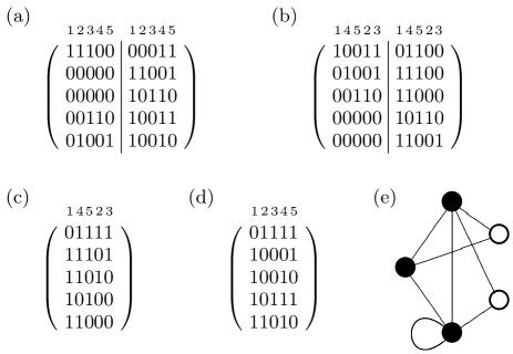
Figure 1: (a) A generator matrix for a stabilizer state. (b) A canonical-form generator matrix obtained from (a) by row and qubit swapping. (c) The adjacency matrix indicated by (b). (d) The adjacency matrix of (c) with the qubit swaps undone. (e) The reduced stabilizer graph associated with (a). In parts (a)-(d) the columns have been labeled by the corresponding qubit. In part (e) the nodes are labeled sequentially, beginning with the top node and moving clockwise. It is clear that the qubit swaps are not actually necessary, since we reverse them in the end. The generator matrix in (a) can be converted to graph form directly by exchanging columns $2$ and $3$ on the left with the matching columns on the right, an operation that corresponds to applying a Hadamard to qubits $2$ and $3$. In graph form, the adjacency matrix is just the right half of the generator matrix. Loops arise from $1$s on the diagonal of the adjacency matrix, and hollow nodes are used to indicate which columns were exchanged between the right and left halves of the generator matrix to get the adjacency matrix. Notice that there are no edges between hollow nodes, nor are there any loops on hollow nodes.

The following steps provide a recipe for translating an arbitrary stabilizer generator matrix into a stabilizer graph:

1. Through row reduction and qubit swapping, transform the generator matrix into canonical form, as in Eq. (3), keeping track during the process of how columns of the generator matrix map to qubits.

2. Draw the graph corresponding to the adjacency matrix

   $$\left(\begin{array}[]{cc}B&A\\ A^{T}&0\end{array}\right)\;,$$ (8)

   including loops for $1$s on the diagonal.

3. Make solid the nodes corresponding to the rows and columns of the submatrix $B$, and make hollow the nodes corresponding to the rows and columns of the submatrix $0$.

Notice that this procedure does not associate every combination of edges, loops, hollow nodes, and solid nodes with a stabilizer state. Because the submatrix $0$ in Eq. (8) contains only $0$s, hollow nodes never have loops, and there are no edges between hollow nodes. We refer to stabilizer graphs having this property as reduced. An example of a generator matrix and an associated reduced stabilizer graph is given in Fig. 1.

It is important to note that the graphs in this paper are labeled graphs in that each node is associated with a particular qubit. Swapping two qubits is a physical operation that generally produces a different quantum state. In our graphs a SWAP gate can be described either by relabeling the corresponding nodes or by exchanging the nodes and all their decorations and connections while leaving the labeling the same. Since the process of bringing the generator matrix into canonical form can involve swapping qubits, we must keep track during this process of the correspondence between qubits and columns of the generator matrix and thus between these columns and the nodes of our graphs.

Just as a generator matrix contains no information about generator signs, so also are stabilizer graphs derived from generator matrices devoid of such information. It is for this reason that we can be cavalier about whether $S$ or $S^{\dagger}=ZS$ is used to convert a canonical generator matrix to strict graph form. In the absence of sign information, however, stabilizer graphs are best thought of as specifying an orthonormal basis rather than a single stabilizer state. Luckily, it is not hard to include sign information in the graph, as we show in the next subsection.

III.2 Graphs from quantum circuits

Having motivated a stabilizer-graph notation using generator matrices, we now turn to the quantum-circuit formalism to expand it. The binary representation of stabilizers lacks a convenient way to keep track of generator signs, applied gates, and qubit swaps. Since, for example, labeling is important, the column exchanges required to bring a generator matrix to canonical form must be tracked, perhaps by appending an extra row with qubit labels to the generator matrix. Details such as this are automatically dealt with when deriving stabilizer graphs from quantum circuits.

Consider a quantum circuit consisting of three layers of gates applied to $N$ qubits, each initially in the state $|0\rangle$. In the first layer, the Hadamard gate, $H$, is applied to each qubit. In the second, controlled-sign gates, ${\vphantom{Z}}^{C}\!{Z}$, are applied between various pairs of qubits. Finally, in the third layer, sign-flip gates, $Z$, phase gates, $S$, and Hadamard gates are applied (in that order) to various subsets of qubits. We refer to such circuits as having graph form.

The descriptor arises because a quantum circuit in this form can be depicted as a graph possessing three kinds of decoration. In such a graph, two nodes are linked if a ${\vphantom{Z}}^{C}\!{Z}$ gate is applied between the qubits of the circuit corresponding to those nodes; the various kinds of node decoration indicate the presence or absence of terminal $Z$, $S$, and $H$ gates on the corresponding qubits. It is the restrictions of such a representation that impel us to specify an order for the terminal gates, since $SH\neq HS$. The decoration corresponding to each gate is as follows: $Z$ gates are denoted by a minus sign in the node, $S$ gates by a loop, and $H$ gates by a hollow (as opposed to a solid) node. We refer to an arbitrary arrangement of solid and hollow nodes with loops, edges, and signs as a stabilizer-state graph or, more simply, as a stabilizer graph. An example graph-form circuit and the corresponding stabilizer graph are given in Fig. 2.

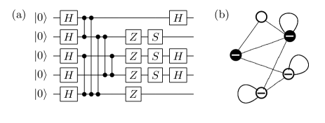
Figure 2: (a) A circuit in graph form. (b) A stabilizer graph corresponding to the circuit in (a). ${\vphantom{Z}}^{C}\!{Z}$ gates between qubits are transformed into links between nodes, terminating $Z$ gates become negative signs, terminating $S$ gates result in loops, and terminating $H$ gates are denoted by hollow nodes. Nodes in (b) are labeled sequentially, beginning with the top node and moving clockwise.

As might be guessed from our choice of decorations, the $Z$ gates in a graph-form circuit specify the signs of the stabilizer generators. The gates applied in the third layer of a graph-form circuit can be written as

$$\prod_{j=1}^{N}H_{j}^{c_{j}}S_{j}^{b_{j}}Z_{j}^{a_{j}}\;,$$ (9)

where $a_{j}$, $b_{j}$, and $c_{j}$ are binary variables taking on the values $0$ or $1$. From Eq. (9) it follows that the third layer of gates transforms a set of graph-state generators as in Eq. (1) to the following stabilizer-state generators:

$$g_{j}= (-1)^{a_{j}+b_{j}c_{j}}$$

$$\times X_{j}^{(b_{j}+1)(c_{j}+1)}Y_{j}^{b_{j}}Z_{j}^{(b_{j}+1)c_{j}}\prod_{k\in\mathcal{N}(j)}Z_{k}^{c_{k}+1}X_{k}^{c_{k}}\;.$$ (10)

Equation (10) shows that the exclusive effect of each terminal $Z$ operator is to flip the sign of a single stabilizer generator. This can also be seen through circuit identities, since pushing a $Z$ gate from the third layer of a graph-form quantum circuit to the beginning of the circuit merely transforms it to an $X$ gate; flipping an input bit is equivalent to flipping the sign of the associated stabilizer since the stabilizer of $|0\rangle$ is $Z$, which acquires a negative sign under conjugation by $X$. Using either of these methods, it is clear that terminal $Z$ gates, and hence the signs in stabilizer graphs, only impact the signs of the stabilizer generators, and can thus be omitted when these signs are thought to be unimportant.

Modulo generator signs, the definition of stabilizer graphs given in the previous subsection and the definition given in this one are compatible. The graph-form circuit and generator matrix associated with a stabilizer graph each specify the same stabilizer up to possible signs. The method of deriving stabilizer graphs from generator matrices described in Sec. III.1, however, produces exclusively reduced stabilizer graphs, i.e., stabilizer graphs satisfying the restriction that hollow nodes never have loops and never be connected to other hollow nodes. In terms of graph-form quantum circuits, this is the restriction that lines with terminating Hadamard gates have no terminating $S$ gates and not be connected by ${\vphantom{Z}}^{C}\!{Z}$ gates. The relative merits of stabilizer graphs and reduced stabilizer graphs are clarified in the following sections, particularly Sec. V. Important roles are found for both.

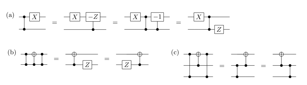
Figure 3: Simple circuit identities, which we use to derive more complex identities. Identity (a) follows trivially from the steps shown. Identities (b) and (c) are easily verified in the standard basis.

IV Graph transformations

It is frequently useful to consider the way in which stabilizer states transform under the application of Clifford gates. Primarily, this is because Clifford gates take stabilizer states to stabilizer states, a property that follows from their preservation of the Pauli group. This same property implies that the action of a Clifford gate can be thought of as a transformation between the graphs representing the initial and final stabilizer states. In this section we consider the transformations induced by local Clifford gates. The transformations induced by ${\vphantom{Z}}^{C}\!{Z}$ gates are discussed separately in the Appendix.

IV.1 Terminology

We begin by introducing terminology for describing transformations on stabilizer graphs. We use a number of terms, some adopted from graph theory and others invented for the task at hand.

Among those terms common to graph theory are neighbors, complement, and local complement. The neighbors of a node $j$ are those nodes connected to $j$ by edges; we denote the set of neighbors of node $j$ by $\mathcal{N}(j)$. In the transformation rules that follow, a loop does not count as an edge, so a node is never its own neighbor. Complementing the edge between two nodes removes the edge if one is present and adds one otherwise. The local complement is performed by complementing a selection of edges, with the pattern of edges depending on whether local complementation is applied to a node or along an edge.

Performing local complementation on a node complements the edges between all of the node’s neighbors. Thus, local complementation at node $j$ transforms the adjacency matrix $\Gamma$ of a graph according to

$$\Gamma_{lm}\rightarrow\Gamma^{\prime}_{lm}=\Gamma_{lm}+(1+\delta_{lm})\Gamma_{jl}\Gamma_{jm}\;;$$ (11)

i.e., it complements an edge if both nodes of the edge are neighbors of $j$.

Local complementation along an edge is equivalent to a sequence of local complementations on the decision nodes, i.e., the nodes defining the edge. The sequence is as follows: first perform local complementation on one of the decision nodes, then local complement on the other decision node, and finally local complement on the first decision node again. This sequence transforms the adjacency matrix of a simple graph in the following way:

$$\Gamma_{lm}\rightarrow\Gamma^{\prime}_{lm} = \Gamma_{lm}+(\Gamma_{jl}+\delta_{jl})(\Gamma_{km}+\delta_{km})$$ (12)

$$\quad{}+(\Gamma_{jm}+\delta_{jm})(\Gamma_{kl}+\delta_{kl})\;,$$

where $j$ and $k$ are the decision nodes. Equation (12) is symmetric in the two decision nodes, so it does not matter at which decision node local complementation is first performed. Additionally, since we do not consider self-loops to be edges, Eq. (12) can be applied to adjacency matrices with nonzero diagonal entries simply by ignoring those entries. Notice that an edge one of whose nodes is a decision node transforms according to $\Gamma^{\prime}_{lj}=\Gamma_{lk}$.

To describe the net effect of local complementation along an edge, it is helpful to define the decision neighborhood of a node as the intersection of its neighborhood with the decision nodes. Then local complementation along an edge can be summarized by three steps:

1. The edge between the decision nodes is left unchanged.

2. An edge one of whose nodes is a decision node is transferred from this decision node to the other.

3. An edge neither of whose nodes is a decision node is complemented if its end nodes have decision neighborhoods that are not empty and not identical.

To these terms we add flip and advance. Flip is used to describe the simple reversal of some binary property, such as the sign or the fill state (color) of a node. Advance refers specifically to an action on loops; advancing generates a loop on nodes where there was not previously one, and it removes the loop and flips the sign on nodes where there was a loop. Its action mirrors the application of the phase gate, since $S^{2}=Z$.

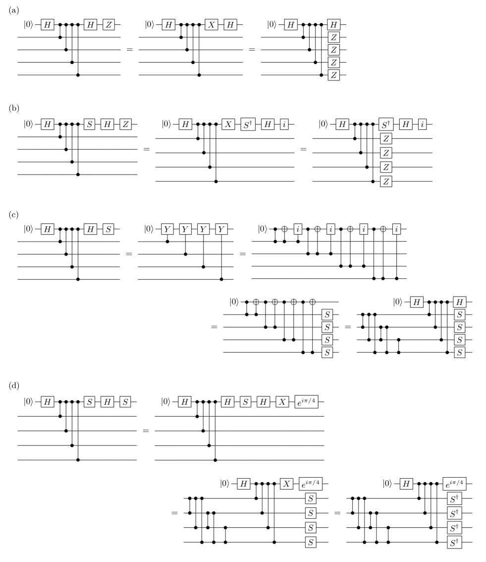
Figure 4: Circuit identities relevant to transforming a stabilizer graph under local Clifford operations. Each identity is illustrated for the case of four neighbors connected to a qubit of interest; equivalent expressions hold for other numbers of neighbors. Identities (a) and (b) follow immediately from the identity in Fig. 3(a). The proof of (c) relies on decomposing ${\vphantom{Y}}^{C}\!{Y}$ using $Y=iXZ$, the equivalence of ${\vphantom{i}}^{C}\!{i}$ to $S$ on the control qubit, and the identity in Fig. 3(c). The first step in identity (d) uses the fact that $I=e^{-i\pi/4}(HS)^{3}$, which gives $SHS=e^{i\pi/4}XHSH$; the second and third steps follow from identities (c) and (a). The identity in Fig. 3(c) generates the thicket of controlled-sign gates in the lower left of the final circuits in (c) and (d), thereby giving rise to local complementation in the corresponding stabilizer graphs. In (b) and (d), the phase shifts on the top qubits, $i$ and $e^{i\pi/4}$, are global phase shifts and thus can be omitted. To complete the transformation rules, it is necessary to know what happens in each of these circuit identities when there is a $Z$ gate on the top qubit immediately after the ${\vphantom{Z}}^{C}\!{Z}$ gates. Ignoring overall phases, the effect on the third layer of the final circuit is, for (a) and (b), to include an additional $Z$ on the top qubit and, for (c) and (d), to include an additional $Z$ on all qubits.

IV.2 Stabilizer-graph transformations

An arbitrary local Clifford operation can be decomposed into a product of $H$, $S$, and $Z$ gates (the $Z$ is unnecessary, but convenient). The effect of a local Clifford operation on a stabilizer graph can thus be obtained by repeated application of the following six transformation rules.

1. Applying $H$ to a node flips its fill.

2. Applying $S$ to a solid node advances its loop.

3. Applying $S$ to a hollow node without a loop performs local complementation on the node and advances the loops of its neighbors.

   If the node has a negative sign, flip the signs of its neighbors as well.

4. Applying $S$ to a hollow node with a loop flips its fill, removes its loop, performs local complementation on it, and advances the loops of its neighbors.

   If the node does not have a negative sign, flip the signs of its neighbors as well.

5. Applying $Z$ to a solid node flips its sign.

6. Applying $Z$ to a hollow node flips the signs of all of its neighbors. If the node has a loop, its own sign is flipped as well.

These transformation rules can be derived from the circuit identities in Fig. 4, which rely on the basic circuit identities given in Fig. 3. Given an understanding of the relationship between circuits and graphs, transformation rules T1, T2, and T5 are trivial. Transformation rule T6 follows simply from Fig. 4(a,b). Transformation rules T3 and T4 derive from Figs. 4(c) and (d), respectively.

IV.3 Reduced-stabilizer-graph transformations

The transformation rules T1–T6 do not generally take reduced stabilizer graphs to reduced stabilizer graphs. From Sec. III.1, however, we know that there exists a reduced stabilizer graph corresponding to each stabilizer state, so it is always possible to represent the effect of a local Clifford operation as a mapping between reduced stabilizer graphs. The appropriate transformation rules for reduced stabilizer graphs are listed below, excepting those for $Z$ operations, which are identical to T5 and T6.

• Applying $H$ to a solid node without a loop, which is only connected to other solid nodes, flips the fill of that node.

• Applying $H$ to a solid node with a loop, which is only connected to other solid nodes, performs local complementation on the node and advances the loops of its neighbors.

  Flip the node’s sign, and if it now has a negative sign, flip the signs of its neighbors as well.

• Applying $H$ to a solid node without a loop, which is connected to a hollow node, flips the fill of the hollow node and performs local complementation along the edge connecting the nodes.

  Flip the sign of nodes connected to both the solid and hollow nodes. If either of these two nodes has a negative sign, flip it and the signs of its current neighbors.

• Applying $H$ to a solid node with a loop, which is connected to a hollow node, performs local complementation on the solid node and then on the hollow node. Then it removes the loop from the solid node, advances the loops of the solid node’s current neighbors, and flips the fill of the hollow node.

  Flip the signs of nodes that were originally connected to both the solid and hollow nodes. If the originally solid node initially had a negative sign, flip it and the signs of its current neighbors, and if the originally hollow node initially had a negative sign, flip the signs of its current neighbors.

• Applying $H$ to a hollow node flips its fill.

• Applying $S$ to a solid node advances its loop.

• Applying $S$ to a hollow node performs local complementation on that node and advances the loops of its neighbors.

  If the node has a negative sign, flip the signs of its neighbors as well.

Of these transformation rules, T(i), T(v), and T(vi) are trivial, and T(vii) is a rewrite of T3. To prove the others requires results from Sec. V, in particular, the equivalence rules in Sec. V.1. Specifically, T(ii) is obtained by applying equivalence rule E1, which gives an equivalent, but unreduced graph and then applying the Hadamard, via rule T1, which leaves a reduced graph. For T(iii), one first applies the Hadamard, via rule T1, and then uses equivalence rule E2 to convert to a reduced graph. In the case of T(iv), one applies the Hadamard, using rule T1, and then applies equivalence rule E1, first to the originally solid node and then to the hollow node. A key part of these transformations is the conversion of stabilizer graphs to reduced form, a process discussed in more detail in Sec. V.3.1.

It is not hard to check that, in using rules T(iii) and T(iv), any other hollow nodes that are connected to the originally solid node do not become connected and do not acquire loops, in accordance with the need to end up with a reduced graph.

V Equivalent stabilizer graphs

As we have defined it, the mapping between a graph-form circuit and its corresponding stabilizer graph is one-to-one. This does not imply, however, that each stabilizer state corresponds to a unique graph. On the contrary, an example of different graph-form circuits corresponding to the same stabilizer state can be found in Fig. 4. Applying an additional $S$ gate to the top qubit in Fig. 4(d) makes the initial circuit identical to that in (b), but the final circuits are quite different. The two circuit identities thus define distinct transformation rules for applying a $Z$ gate to a hollow node with a loop, thereby demonstrating the existence of multiple, equivalent graph-form circuits. For every way of obtaining a particular stabilizer state from a circuit in graph form, there is an associated stabilizer graph. In this section we examine the resulting equivalence classes of stabilizer graphs, first by presenting equivalence rules for full and reduced stabilizer graphs and then by introducing simplified graph-form-circuit equalities which we use to show that the equivalence rules given here are complete.

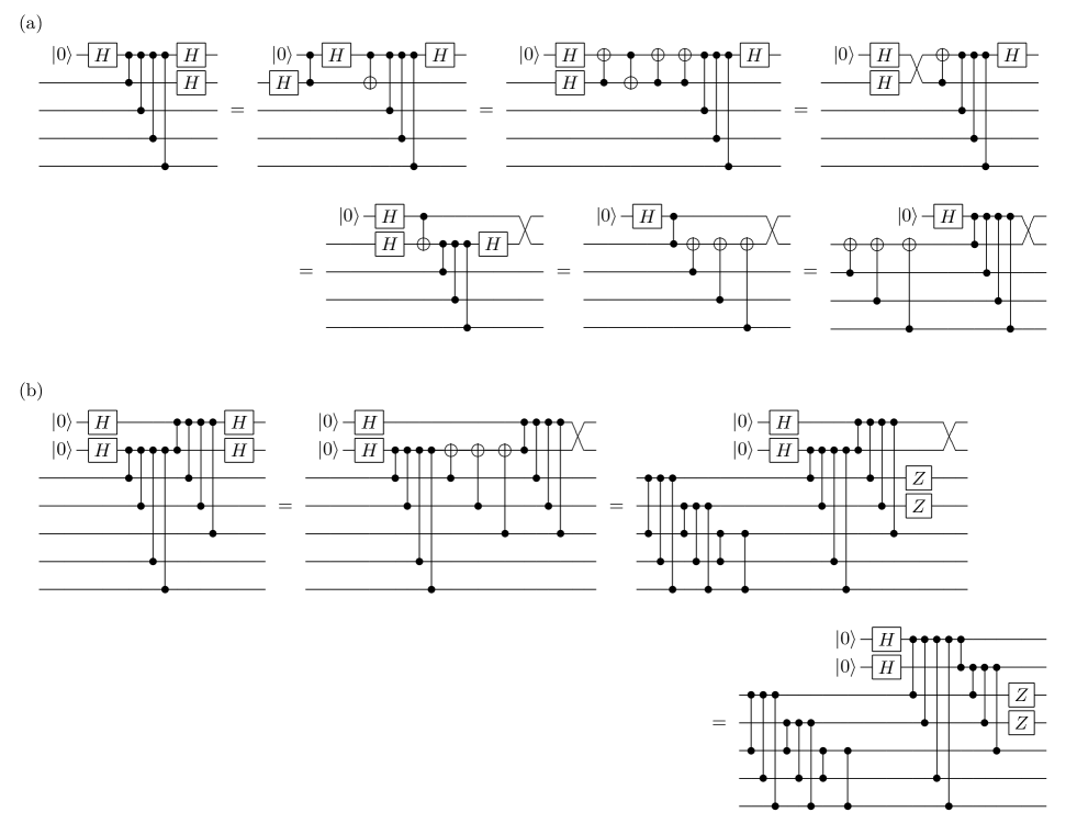
Figure 5: (a) An illustration of a circuit identity used in the removal of pairs of Hadamards. The identity is shown for the case of four neighbors connected to a qubit of interest; equivalent expressions hold for other numbers of neighbors. The crucial trick here is the use of the decomposition of SWAP in terms of three ${\vphantom{X}}^{C}\!{X}$ gates. (b) A circuit identity demonstrating transformation rule E2. The selection of neighbors of the top two qubits, the decision qubits, is chosen to display the behavior of all kinds of edges in which both end nodes are connected to at least one of the decision qubits. The first equality in (b) employs the identity from part (a), while the subsequent ones follow from basic circuit identities. Concerning edges, the net effect of E2 on a stabilizer graph is to perform local complementation along the edge joining the decision nodes, i.e., to swap the connections of the decision nodes and to complement any edges whose end nodes connect to the decision nodes in different ways. The latter of these effects is contained in the controlled-sign gates in the lower left of the final circuit. Circuits illustrating E2 for other initial fill states can be obtained simply by applying additional terminal Hadamards to the circuits in (b). The sign rule for E2 expresses the effect of a $Z$ gate on a decision qubit before the Hadamard gate in the third layer of the initial circuit. Such a $Z$ gate can be pushed through the succeeding Hadamard, becoming an $X$ gate; in the final circuit, this $X$ gate, when processed using the identity in Fig. 3(a), deposits an additional $Z$ gate on the qubits that were originally connected to the other decision qubit, excluding the decision qubit that originally possessed the $Z$.

V.1 Stabilizer-graph equivalences

Applying either of the following two rules to a stabilizer graph yields an equivalent graph, i.e., one which represents the same stabilizer state.

1. Flip the fill of a node with a loop. Perform local complementation on the node, and advance the loops of its neighbors.

   Flip the node’s sign, and if the node now has a negative sign, flip the signs of its neighbors as well.

2. Flip the fills of two connected nodes without loops, and local complement along the edge between them.

   Flip the signs of nodes connected to both of the two original nodes. If either of the two original nodes has a negative sign, flip it and the signs of its current neighbors.

The first of these equivalence rules can be obtained by applying an additional $S$ gate to the top qubit in the identity of Fig. 4(d) and equating the final circuit to the final circuit in Fig. 4(b). For the second rule, we need yet another circuit identity. Figure 5(a) shows how Hadamards can be removed from a pair of connected qubits without $S$ gates. Figure 5(b) extends this identity to a demonstration of rule E2.

V.2 Reduced-stabilizer-graph equivalences

The equivalence rules of the previous section can be reworked to yield equivalence rules for reduced stabilizer graphs. The resulting equivalence rules are

• For a hollow node connected to a solid node with a loop, local complement on the solid node and then on the hollow node. Then remove the loop from the solid node, advance the loops of its current neighbors, and flip the fills of both nodes.

  As for signs, follow the sequence in transformation rule T(iv).

• For a hollow node connected to a solid node without a loop, local complement along the edge between them. Then flip the fills of both nodes.

  As for signs, follow the sequence in equivalence rule E2.

There is a simple relationship between the two sets of equivalence rules. Equivalence rule E(ii) is identical to E2 for the case that the two connected nodes have opposite fill. Equivalence rule E(i) is simply rule E1 applied twice: first to the solid node with the loop and then once to the hollow node that has acquired a loop from the first application of E1. The second application of E1 is needed because the resulting graph is not reduced after one employment of the rule.

Both of these equivalence rules can also be derived by applying two Hadamards to a solid node, E(i) handling the case in which the solid node has a loop and E(ii) the case in which it does not. Thus equivalence rule E(i) is simply transformation rule T(iv) followed by use of rule T(i) to apply a second Hadamard to the originally solid node. Likewise, E(ii) is rule T(iii) followed by T(i) to apply a second Hadamard to the originally solid node. Notice that both rules preserve the number of hollow nodes.

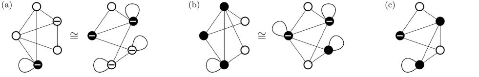
Figure 6: An example sequence of graphs representing parts $1$ through $3$ of the equivalence-checking procedure in Sec. V.3. Nodes are labeled sequentially, beginning at the top node and moving clockwise. The graph on the left-hand side of (a) is equivalent to the reduced graph on the left-hand side of (b) by the application of E2 to the pair of nodes $\{1,5\}$. Likewise, an application of E1 to node $3$ in the graph on the right-hand side of (a) yields the reduced graph on the right-hand side of (b). The graph of (c) results from the application of E(ii) to the pair of nodes $\{1,2\}$ in the graph on the left of (b). An application of E(i) to the pair of nodes $\{3,4\}$ in the graph on the right-hand side of (b) also yields the graph in (c), verifying, as per Sec. V.3.3, that the graphs in (a) represent the same state.

V.3 Constructive procedure for showing sufficiency of equivalence rules

Having described a set of rules for converting between equivalent stabilizer graphs, we show in this section that, in each case, the aforementioned rules generate the entire equivalence class of stabilizer graphs. The proof is divided into three parts. The first part shows how to use rules E1 and E2 to convert an arbitrary stabilizer graph to an equivalent graph in reduced form. The second part explains how an equivalence test for a pair of reduced stabilizer graphs can be simplified, using rules E(i) and E(ii), to a special form. Finally, the third part proves that the graphs on the two sides of such a simplified equivalence test are equivalent only if they are trivially identical. Taken as a whole, this proves that the set of equivalence rules given in Secs. V.1 and V.2 is sufficient to convert (reversibly) between any two equivalent stabilizer graphs and thus that they generate all stabilizer graphs that are equivalent to the same stabilizer state. Similarly, considering only the final two parts of the proof shows that the rules given in Sec. V.2 are sufficient to generate all reduced stabilizer graphs.

V.3.1 Converting stabilizer graphs to reduced form

Two features identify a stabilizer graph as reduced. In a reduced graph, hollow nodes never have loops, and hollow nodes are never connected to each other. Equivalence rule E1 can be used to convert looped nodes from hollow to solid. Applying rule E1 in this sort of situation can cause hollow nodes to acquire loops, but each application fills one hollow node of the graph, so the procedure will terminate in at most a number of repetitions equal to the number of hollow nodes in the graph. Similarly, connected hollow nodes in the resulting graph can be converted to solid nodes using the appropriate case of rule E2. Once again, the process is guaranteed to terminate because the number of hollow nodes to which the rule might be applied decreases by two with each application of the rule. Concomitantly, the conversion of a stabilizer graph to an equivalent reduced graph never increases the number of hollow nodes.

V.3.2 Simplifying reduced-graph equivalence testing

Equivalence testing for pairs of reduced graphs is facilitated by simplifying the equivalence such that nodes that are hollow only in the first graph never connect to nodes that are hollow only in the second. This simplification can be accomplished by iterating the following process. Choose a pair of connected (in either graph) nodes $a$ and $b$ such that $a$ is hollow in one graph and $b$ is hollow in the other, and to the graph in which they are connected, apply the relevant reduced equivalence rule to the selected nodes. Among other things, the equivalence operation reverses the fill of the two nodes it is applied to. Since one node is hollow and the other solid, this preserves the total number of hollow nodes while yielding a node that is hollow in both graphs. Because it is applied only to unpaired hollow nodes, subsequent uses of this equivalence rule do not disturb the newly paired hollow node. Consequently, this process also terminates in at most a number of repetitions equal to the number of hollow nodes in each of the graphs.

V.3.3 Trivial evaluation of simplified reduced-graph
equivalence tests

The two reduced graphs composing a simplified reduced-graph equivalence test are equivalent, i.e., correspond to the same state, if and only if the graphs are identical. To see why this is so, we return to the graph-form quantum circuits discussed earlier. In addition to the standard restrictions for reduced graphs, the circuits corresponding to the graphs in a simplified equivalence test have the following property: if in one of the circuits, a qubit with a terminal $H$ participates in a ${\vphantom{Z}}^{C}\!{Z}$ gate with a second qubit (which cannot have a terminal $H$), then in the other circuit, it cannot be true that the second qubit has a terminal $H$ and the first does not. We prove the triviality of simplified reduced-graph equivalence testing by considering an arbitrary simplified reduced-graph equivalence test and showing that the two graphs must be identical if they are to correspond to the same state.

In terms of unitaries, an arbitrary graph-form circuit equality can be written as

$$\begin{split}\prod_{g\in\mathcal{H}_{l}}&H_{g}\prod_{j\in\mathcal{S}_{l}}S_{j}\prod_{h\in\mathcal{Z}_{l}}Z_{h}\prod_{\gamma\in\mathcal{C}_{l}}{\vphantom{Z}}^{C}\!{Z}_{\gamma}\prod_{k}H_{k}|0\rangle^{\otimes n}\\ =&\prod_{g\in\mathcal{H}_{r}}H_{g}\prod_{j\in\mathcal{S}_{r}}S_{j}\prod_{h\in\mathcal{Z}_{r}}Z_{h}\prod_{\gamma\in\mathcal{C}_{r}}{\vphantom{Z}}^{C}\!{Z}_{\gamma}\prod_{k}H_{k}|0\rangle^{\otimes n}\;,\end{split}$$ (13)

where $\mathcal{C}$ lists the pairs of qubits participating in ${\vphantom{Z}}^{C}\!{Z}$ gates and $\mathcal{H}$, $\mathcal{Z}$, and $\mathcal{S}$ are sets enumerating the qubits to which $H$, $Z$, and $S$ gates are applied respectively. The total number of qubits is denoted by $n$ and the subscripts $l$ and $r$ discriminate between the circuits on the left- and right-hand sides of the equation. In terms of these sets, a reduced-graph-form circuit satisfies the constraints $\mathcal{H}\cap\mathcal{S}=\varnothing$ and $\{a,b\}\not\in\mathcal{C}$ for all $a,b\in\mathcal{H}$. The circuits in simplified tests also satisfy $\{a,b\}\not\in\mathcal{C}_{l},\mathcal{C}_{r}$ for all $a\in\mathcal{H}_{l}\cap\overline{\mathcal{H}}_{r}$ and $b\in\overline{\mathcal{H}}_{l}\cap\mathcal{H}_{r}$, where $\bar{\mathcal{H}}$ denotes the complement of $\mathcal{H}$, i.e., the set of qubits to which $H$ is not applied.

Suppose now that the two graphs have hollow nodes at different locations; i.e., at least one of the sets, $\mathcal{H}_{l}\cap\overline{\mathcal{H}}_{r}$ and $\overline{\mathcal{H}}_{l}\cap\mathcal{H}_{r}$, is not empty. For specificity, let’s say that $\mathcal{H}_{l}\cap\overline{\mathcal{H}}_{r}$ is not empty. In the language of circuits, this means that there exists a qubit $a$ that has a terminal $H$ on the left side of Eq. (13), but not on the right side. Since qubit $a$ is part of a circuit for a reduced graph, it does not participate in ${\vphantom{Z}}^{C}\!{Z}$ gates with other qubits that possess terminal $H$ gates. Consequently, on the left side of Eq. (13), the ${\vphantom{Z}}^{C}\!{Z}$ gates involving qubit $a$ can all be moved to the end of the circuit where they become ${\vphantom{X}}^{C}\!{X}$ gates with $a$ as the target. Doing this and transferring the ${\vphantom{X}}^{C}\!{X}$ gates to the other side yields,

$$\begin{split}\prod_{g\in\mathcal{H}_{l}}H_{g}\prod_{j\in\mathcal{S}_{l}}S_{j}\prod_{h\in\mathcal{Z}_{l}}Z_{h}\prod_{\gamma\in\mathcal{C}_{l}\mbox{\scriptsize{\ s.t.\ }}a\not\in\gamma}\!\!\!\!\!{\vphantom{Z}}^{C}\!{Z}_{\gamma}\;\;\prod_{k}H_{k}|0\rangle^{\otimes n}=\prod_{b\in\mathcal{N}_{l}(a)}{\vphantom{X}}^{C}\!{X}_{ba}\prod_{g\in\mathcal{H}_{r}}H_{g}\prod_{j\in\mathcal{S}_{r}}S_{j}\prod_{h\in\mathcal{Z}_{r}}Z_{h}\prod_{\gamma\in\mathcal{C}_{r}}{\vphantom{Z}}^{C}\!{Z}_{\gamma}\prod_{k}H_{k}|0\rangle^{\otimes n}\;,\end{split}$$ (14)

where $\mathcal{N}_{l}(a)$ denotes the set of qubits that participate in ${\vphantom{Z}}^{C}\!{Z}$ gates with qubit $a$ on the left-hand side of Eq. (13).

Because the original graph equality (13) was simplified, $\mathcal{N}_{l}(a)\cap\mathcal{H}_{r}=\varnothing$ and, by assumption, $a\not\in\mathcal{H}_{r}$, so the ${\vphantom{X}}^{C}\!{X}$ gates and the terminal Hadamards on the right side of Eq. (14) do not act on the same qubits. Thus we can commute the ${\vphantom{X}}^{C}\!{X}$ gates past the terminal Hadamards. Moreover, we can then move the ${\vphantom{X}}^{C}\!{X}$ gates to the beginning of the circuit where they have no effect and can therefore be dropped. During this migration, however, they generate a complicated menagerie of phases. The resulting expression for the right side of Eq. (14) is

$$\begin{split}\prod_{g\in\mathcal{H}_{r}}H_{g}\prod_{j\in\mathcal{S}_{r}}S_{j}\raisebox{-3.50006pt}{\Bigg{(}\Bigg{.}}\prod_{d\in\mathcal{N}_{l}(a)}S_{d}{\vphantom{Z}}^{C}\!{Z}_{da}\raisebox{-3.50006pt}{\Bigg{.}\Bigg{)}}^{\!\!\mathbf{1}_{\mathcal{S}_{r}}(a)}\prod_{h\in\mathcal{Z}_{r}}Z_{h}\raisebox{-3.50006pt}{\Bigg{(}\Bigg{.}}\prod_{f\in\mathcal{N}_{l}(a)}Z_{f}\raisebox{-3.50006pt}{\Bigg{.}\Bigg{)}}^{\!\!\mathbf{1}_{\mathcal{Z}_{r}}(a)}\prod_{\gamma\in\mathcal{C}_{r}}{\vphantom{Z}}^{C}\!{Z}_{\gamma}\prod_{\delta\in\mathcal{N}(a)}{\vphantom{Z}}^{C}\!{Z}_{\delta}\prod_{c\in\mathcal{N}_{l}(a)\cap\mathcal{N}_{r}(a)}\!\!\!Z_{c}\;\;\prod_{k}H_{k}|0\rangle^{\otimes n}\;,\end{split}$$ (15)

where $\mathcal{N}_{r}(a)$ is defined similarly to $\mathcal{N}_{l}(a)$,

$$\mathcal{N}(a)=\{\{p,q\}|p\in\mathcal{N}_{l}(a),q\in\mathcal{N}_{r}(a),p\neq q\}\;,$$ (16)

and $\mathbf{1}$ represents an indicator function, e.g., $\mathbf{1}_{\mathcal{Z}_{r}}(a)$ equals $1$ if $a\in\mathcal{Z}_{r}$ and $0$ otherwise.

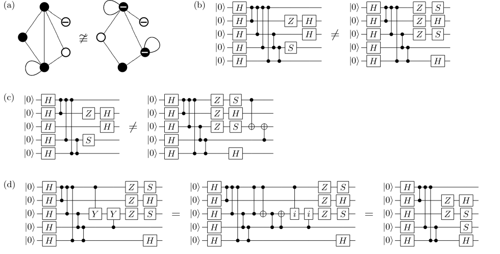
Figure 7: An example of the process described in Sec. V.3.3. A simplified reduced-graph equivalence test is shown in (a). The test is simplified because a node that is hollow in only one graph is never connected to a node that is hollow only in the other. The test is also false, since such an equivalence is satisfied if and only if the two graphs are identical. By switching to circuit notation, it is possible to see why these graphs correspond to different states. Translating the graph equality in (a) into circuit notation yields the circuit equality in (b), where the nodes of (a) are taken to be numbered sequentially, beginning at the top node and moving clockwise. The fact that the graphs are reduced implies that qubits with terminal $H$ gates, such as qubit $3$ in the left-hand circuit, are not connected to other qubits with terminal $H$ gates. This allows us to pull out the ${\vphantom{Z}}^{C}\!{Z}$ gates acting on qubit $3$ on the left side and transfer the resulting ${\vphantom{X}}^{C}\!{X}$ gates to the other side of the equation, yielding the equality in (c). That the graph equality was simplified guarantees that $H$ gates do not prevent us from then pushing the ${\vphantom{X}}^{C}\!{X}$ gates to the beginning of the right-hand circuit in (c), as shown in (d). Qubit 3 winds up separable on both sides of the equation (though this is not generally the case), allowing us to verify the inequivalence of the prepared states since $|0\rangle\neq(|0\rangle-i|1\rangle)/\sqrt{2}$.

It might appear that we have made things substantially worse by this rearrangement, but in an important sense, Eq. (15) is now very simple with regard to qubit $a$: $H$ is applied to qubit $a$ followed by a sequence of unitary gates all of which are diagonal in the standard basis. This implies that there are an equal number of terms in the resultant state where qubit $a$ is in the state $|0\rangle$ and the state $|1\rangle$. On the left side of Eq. (14), however, the only gate remaining on qubit $a$ is the identity or an $X$, depending on whether $a\in\mathcal{Z}_{l}$; thus qubit $a$ is separable and is either in state $|0\rangle$ or $|1\rangle$ depending on whether $a\in\mathcal{Z}_{l}$. Consequently, our initial assumption that $\mathcal{H}_{l}\neq\mathcal{H}_{r}$ is incompatible with satisfying the equality.

The preceding discussion shows that two graphs composing a simplified equivalence test are equivalent only if they have hollow nodes in exactly the same locations. Given this constraint, the terminal Hadamards can be canceled from both sides of Eq. (13), giving

$$\begin{split}\prod_{h\in\mathcal{Z}_{l}}&Z_{h}\prod_{j\in\mathcal{S}_{l}}S_{j}\prod_{\gamma\in\mathcal{C}_{l}}{\vphantom{Z}}^{C}\!{Z}_{\gamma}\prod_{k}H_{k}|0\rangle^{\otimes n}\\ =&\prod_{h\in\mathcal{Z}_{r}}Z_{h}\prod_{j\in\mathcal{S}_{r}}S_{j}\prod_{\gamma\in\mathcal{C}_{r}}{\vphantom{Z}}^{C}\!{Z}_{\gamma}\prod_{k}H_{k}|0\rangle^{\otimes n}\;.\ \end{split}$$ (17)

The state after the initial Hadamards is an equally weighted superposition of all the states in the standard basis. The subsequent unitaries are diagonal in the standard basis, so they put various phases in front of the terms in the equal superposition. Since a unitary is fully described by its action on a complete set of basis states, demanding equality term-by-term in Eq. (17) amounts to requiring that

$$\prod_{h\in\mathcal{Z}_{l}} Z_{h}\prod_{j\in\mathcal{S}_{l}}S_{j}\prod_{\gamma\in\mathcal{C}_{l}}{\vphantom{Z}}^{C}\!{Z}_{\gamma}=\prod_{h\in\mathcal{Z}_{r}}Z_{h}\prod_{j\in\mathcal{S}_{r}}S_{j}\prod_{\gamma\in\mathcal{C}_{r}}{\vphantom{Z}}^{C}\!{Z}_{\gamma}\;,$$ (18)

which is only satisfied when $\mathcal{Z}_{l}=\mathcal{Z}_{r}$, $\mathcal{S}_{l}=\mathcal{S}_{r}$, and $\mathcal{C}_{l}=\mathcal{C}_{r}$. Thus, after simplification, the equivalence of pairs of reduced graphs is trivial to evaluate, since equivalence requires that the two graphs be identical.

An example of the entire process of testing graph equivalence is given in Fig. 6. An example which illustrates the circuit manipulations described algebraically in the text of this section is given in Fig. 7.

As mentioned above, our proof provides a constructive procedure for testing the equivalence of stabilizer graphs. Moreover, it shows that the set of equivalence rules given in Sec. V.1 is sufficient to convert between any equivalent stabilizer graphs and that the rules given in Sec. V.2 are sufficient to convert between any equivalent reduced stabilizer graphs. Since the conversion of an arbitrary stabilizer graph to reduced form never increases the number of hollow nodes and the rules E(i) and E(ii) that convert among reduced graphs preserve the number of hollow nodes, we conclude that the reduced stabilizer graphs for a stabilizer state are those that have the least number of hollow nodes.

VI Conclusion

Motivated by the relation between the graphs and the generator matrices associated with graph states, we extend the graph representation of states to encompass all stabilizer states. These stabilizer graphs differ from the graphs employed by hein in that nodes can be either hollow or solid and can possess both loops and signs. The additional decorations identify the local Clifford operations that relate the desired stabilizer state to the graph state corresponding to the unadorned graph. Imposing the restriction that the number of hollow nodes be minimal yields a subset of the stabilizer graphs which we term reduced. Reduced graphs follow naturally from the binary representation of the stabilizer formalism, while generic stabilizer graphs are more closely related to the quantum-circuit formalism. For graph states, reduced stabilizer graphs are identical to the standard representation of these states in terms of graphs.

Using circuit identities, we derive a set of rules for transforming stabilizer graphs under the application of various local Clifford gates. From this list, we abstract a similar set for transforming reduced stabilizer graphs. Considering these transformation rules, particularly those for reduced stabilizer graphs, it becomes clear that the mapping between stabilizer states and stabilizer graphs is not one-to-one. Rules for converting between equivalent graphs are found, and we prove that the equivalence rules given are universal by developing a constructive procedure for testing the equivalence of any two stabilizer graphs.

Appendix A Controlled-$Z$ gates

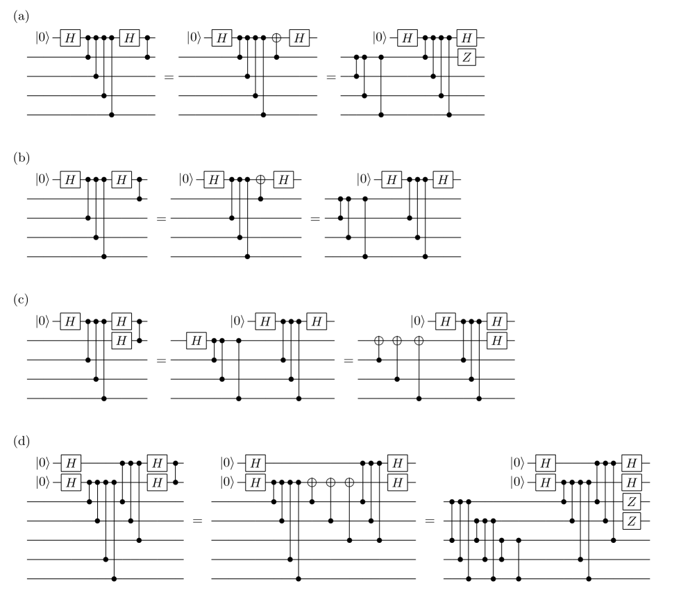
Figure 8: Circuit identities for transforming a reduced stabilizer graph under ${\vphantom{Z}}^{C}\!{Z}$ gates. In (a)–(c) the identity is illustrated for the case of four neighbors connected to a qubit of interest; equivalent expressions hold for other numbers of neighbors. Identities (a) and (b) give the rule T(ix) for transforming a reduced graph when a ${\vphantom{Z}}^{C}\!{Z}$ gate is applied to a hollow node and a solid node. The effect of a $Z$ gate on the hollow qubit in the third layer of (a) or (b) is to deposit an additional $Z$ gate on both the hollow and solid qubits in the third layer of the final circuit. The identity in (c) relies on (b); this identity is extended in (d) to a demonstration of the rule T(x) for transforming a reduced graph when a ${\vphantom{Z}}^{C}\!{Z}$ gate is applied to two hollow nodes. If there is a $Z$ gate on the lower hollow qubit in the third layer of (c), the result in the third layer of the final circuit is to put a $Z$ gate on that qubit and on the neighbors of the other hollow qubit. Translated to (d), this means that a $Z$ gate in the third layer on either hollow qubit leads in the third layer of the final circuit to additional $Z$ gates on that qubit and on the neighbors of the other hollow qubit.

The transformation rules given in Sec. IV suffice to describe the effect of any local Clifford operation on a stabilizer state. In order to complete the set of transformation rules for the Clifford group, we include transformation rules for the ${\vphantom{Z}}^{C}\!{Z}$ gate here. In the interest of brevity, we consider only reduced-stabilizer-graph transformations. Transformation rules for general stabilizer graphs can be derived by first using the equivalence rules in Sec. V.1 to convert to an equivalent reduced graph and then applying the transformation rules below.

• Applying ${\vphantom{Z}}^{C}\!{Z}$ between two solid nodes complements the edge between them.

• Applying ${\vphantom{Z}}^{C}\!{Z}$ between a hollow node and a solid node complements the edges between the solid node and the neighbors of the hollow node.
  
  Flip the solid node’s sign if the two nodes were initially connected and the hollow node did not have a sign or if the two nodes were not connected and the hollow did have a sign.

• Applying ${\vphantom{Z}}^{C}\!{Z}$ between two hollow nodes effects the third step of local complementation along the (unoccupied) edge between the two nodes.

  Nodes that neighbor both decision nodes flip their signs. If a decision node initially had a sign, flip the signs of nodes connected to the other decision node.

Transformation rule T(viii) is trivial since the ${\vphantom{Z}}^{C}\!{Z}$ gate simply commutes into layer two of the reduced-graph-form circuit. The circuit identities needed to prove rules T(ix) and T(x) are given in Fig. 8.

References

- (1) D. Gottesman, PhD thesis, Caltech (1997).
- (2) R. Raussendorf and H. J. Briegel, Phys. Rev. Lett. 86, 5188 (2001).
- (3) M. Van den Nest, J. Dehaene, B. De Moor, Phys. Rev. A 71, 062323 (2005).
- (4) M. Van den Nest, J. Dehaene, and B. De Moor, Phys. Rev. A 69, 022316 (2004).
- (5) R. Diestel, Graph Theory (Springer-Verlag, New York, 2000).
- (6) M. A. Nielsen and I. L. Chuang, Quantum Computation and Quantum Information (Cambridge University Press, Cambridge, England, 2000), Sec. 10.5.3.
- (7) D. Gottesman, Phys. Rev. A 57, 127 (1998).
- (8) S. Aaronson and D. Gottesman, Phys. Rev. A 70, 052328 (2004).
- (9) M. Hein, W. Dür, J. Eisert, R. Raussendorf, M. Van den Nest, and H.-J. Briegel, in Entanglement in Graph Staes and its Applications, Proceedings of the International School of Physics “Enrico Fermi,” Course 162, Varenna, July 5–15, 2005, edited by G. Casati, D. L. Shepelyansky, P. Zoller, and G. Benenti (IOS Press, Amsterdam, 2006), e-print arXiv:quant-ph/0602096.