Robust Quantum Error Correction via Convex Optimization

Abstract

We present a semidefinite program optimization approach to quantum error correction that yields codes and recovery procedures that are robust against significant variations in the noise channel. Our approach allows us to optimize the encoding, recovery, or both, and is amenable to approximations that significantly improve computational cost while retaining fidelity. We illustrate our theory numerically for optimized 5-qubit codes, using the standard [5,1,3] code as a benchmark. Our optimized encoding and recovery yields fidelities that are uniformly higher by 1-2 orders of magnitude against random unitary weight-2 errors compared to the [5,1,3] code with standard recovery. We observe similar improvement for a 4-qubit decoherence-free subspace code

Introduction.— Quantum error correction (QEC) is essential for the scale-up of quantum information devices. A theory of quantum error correcting codes has been developed, in analogy to classical coding for noisy channels Shor:95Gott:96Steane:96 ; Laflamme:96 ; KnillL:97 ; NielsenC:00 . This theory allows one to find perfect-fidelity encoding and recovery procedures for a wide class of noise channels. While it has led to many breakthroughs, this approach has two important disadvantages: (1) Robustness: Perfect QEC schemes, as well those produced by optimization tuned to specific errors, are often not robust to even small changes in the noise channel. (2) Cost: The encoding and recovery effort in perfect QEC typically grows exponentially with the number of errors in the noise channel. Here we present an optimization approach to QEC that addresses both these problems. Regarding robustness, we develop an approach that incorporates specific models of noise channel uncertainty, resulting in highly robust error correction. Thus entire classes of noise channels which do not satisfy the standard assumptions for perfect correction Shor:95Gott:96Steane:96 ; Laflamme:96 ; KnillL:97 ; NielsenC:00 , can be tailored with optimized encoding and/or recovery. Regarding cost, if the resulting robust fidelity levels are sufficiently high, then no further increases in codespace dimension and/or levels of concatenation are necessary. This assessment, which is critical to any specific implementation, is not knowable without performing the robust optimization.

Relation to prior work.— An optimization approach to QEC was reported in a number of recent papers ReimpellW:05 ; YamamotoHT:05FletcherSW:06ReimpellWA:06 ; KosutL:06 . In these works error correction design was posed as an optimization problem to directly maximize fidelity, with the design variables being the process matrices associated with the encoding and/or recovery channels. Here we present an indirect approach to fidelity maximization based on minimizing the error between the actual channel and the desired channel. Both the direct and indirect approaches lead naturally to bi-convex optimization problems, specifically, two semidefinite programs (SDPs) BoydV:04 which can be iterated between recovery and encoding. For a given encoding the problem is convex in the recovery. For a given recovery, the problem is convex in the encoding. However, the indirect approach is in general more efficient computationaly then the direct approach and, as we will show, has the added advantage of incorporating an approximation method which provides a considerable reduction in computational cost with only a minimal fidelity loss.

Organization.— After reviewing the standard error correction model and defining performance measures, we state the direct and indirect fidelity optimization problems, then show how to add robustness measures, and describe methods to solve the (robust) indirect problem. We present a range of examples illustrating the robustness of our codes against increasingly more challenging noise channels, and conclude with a discussion and summary of computational cost.

Noise and error correction model.— Subject to standard assumptions, the dynamics of any open quantum system can be described in terms of a completely-positive (CP) map: $\rho_{S}\to\sum_{i}A_{i}\rho_{S}A_{i}^{\dagger}$, a result known as the Kraus Operator Sum Representation (OSR) NielsenC:00 . Here $\rho_{S}$ is the initial system density matrix and the $A_{i}$ are called operation elements, and satisfy $\sum_{i}A_{i}^{\dagger}A_{i}=I_{S}$ (identity). The standard error correction procedure involves CP encoding (${\mathcal{C}}$), error (${\mathcal{E}}$), and recovery (${\cal R}$) maps (or channels): $\rho_{S}\overset{{\mathcal{C}}}{\to}\rho_{C}\overset{{\mathcal{E}}}{\to}\sigma_{C}\overset{{\cal R}}{\to}\hat{\rho}_{S}$, i.e., using the OSR: $\hat{\rho}_{S}=\sum_{r,e,c}(R_{r}E_{e}C_{c})\rho_{\rm S}(R_{r}E_{e}C_{c})^{\dagger}$ (see Ref. SL:07 for a relaxation of the CP map condition). The encoding $\{C_{c}\}_{c=1}^{m_{C}}$ and recovery $\{R_{r}\}_{r=1}^{m_{R}}$ operation elements are rectangular matrices, respectively ${n_{C}}\times{n_{S}}$ and ${n_{S}}\times{n_{C}}$, since they map between the system Hilbert space (of dimension $n_{S}$) and the system+ancillae Hilbert space (of dimension $n_{C}$). The error $\{E_{e}\}_{e=1}^{m_{E}}$ operation elements are square $({n_{C}}\times{n_{C}})$ matrices, and represent the effects of decoherence and noise. As in KnillL:97 , we will restrict attention to unitary encoding: ${\mathcal{C}}$ has only a single OSR element, the ${n_{C}}\times{n_{S}}$ encoding matrix $C$, whose ${n_{S}}$ columns are the orthonormal codewords ($C^{\dagger}C=I_{S}$) with ${n_{C}}={n_{S}}{n_{CA}}$, ${n_{CA}}$ being the dimension of the encoding ancilla space. It follows from $\rho_{S}={\rm Tr}_{CA,RA}[U_{R}(|0\rangle\langle 0|_{RA}\otimes\sigma_{C})U_{R}^{\dagger}]$, where $U_{R}$ is the unitary recovery acting on the noisy encoded state $\sigma_{C}$ and the recovery ancillae $|0\rangle_{RA}$, that ${m_{R}}={n_{CA}}{n_{RA}}$, with ${n_{RA}}$ the dimension of the recovery ancillae space.

Performance measures.— Our error correction objective is to design the encoding ${\mathcal{C}}$ and recovery ${\cal R}$ so that, for a given ${\mathcal{E}}$, the map $\rho_{S}\to\hat{\rho}_{S}$ is as close as possible to a desired ${n_{S}}\times{n_{S}}$ unitary $L_{S}$. A common measure of performance is the average fidelity between the channel ${\cal R}{\mathcal{E}}{\mathcal{C}}$ and the ideal $L_{S}$: $f_{\rm avg}=\frac{1}{n_{s}^{2}}\sum_{r,e}\ |{\bf Tr}\ L_{S}^{\dagger}R_{r}E_{e}C|^{2}$. $f_{\rm avg}=1$ if and only if there are constants $\alpha_{re}$ such that KnillL:97 ; NielsenC:00 : $R_{r}E_{e}C=\alpha_{re}L_{S},\ \sum_{r,e}|\alpha_{re}|^{2}=1$. This suggests the indirect measure of fidelity, the “distance-like” error (using the Frobenius norm, $\|X\|_{\rm fro}^{2}={\bf Tr}\ X^{\dagger}X$),

$$\begin{array}[]{rcl}d_{\rm ind}&=&\sum_{r,e}\ \|R_{r}E_{e}C_{c}-\alpha_{re}L_{S}\|_{\rm fro}^{2}\\ &=&\|RE(I_{E}\otimes C)-\alpha\otimes L_{S}\|_{\rm fro}^{2}\end{array}$$ (1)

with $\alpha$ the ${n_{CA}}{n_{RA}}\times{m_{E}}$ matrix with elements $\alpha_{re}$, $E$ the ${n_{C}}\times{n_{C}}{m_{E}}$ rectangular error system matrix $E=[E_{1}\ \cdots\ E_{m_{E}}],$ and $R$ the ${n_{C}}{n_{RA}}\times{n_{C}}$ recovery matrix obtained by stacking the ${n_{CA}}{n_{RA}}$ matrices $R_{r}$. Hence, we have $\|\alpha\|_{\rm fro}^{2}={\bf Tr}\ \alpha^{\dagger}\alpha=\sum_{r,e}|\alpha_{re}|^{2}=1$, and $R^{\dagger}R=\sum_{r}\ R_{r}^{\dagger}R_{r}=I_{C}$. Note that $U_{R}=[R|W]$, where $U_{R}$ is the unitary recovery and $W$ is ${n_{C}}{n_{RA}}\times({n_{C}}{n_{RA}}-{n_{C}})$.

As $f_{\rm avg}$ and $d_{\rm ind}$ are explicitly dependent on the channel elements, they are convenient for optimization. Consider then the following optimization problems.

$$\begin{array}[]{c}\mbox{\em Direct Fidelity Maximization}\\ \begin{array}[]{ll}\mbox{maximize}&f_{\rm avg}=\frac{1}{n_{s}^{2}}\sum_{r,e}\ |{\bf Tr}\ L_{S}^{\dagger}R_{r}E_{e}C|^{2}\\ \mbox{subject to}&R^{\dagger}R=I_{C},\;\;C^{\dagger}C=I_{S}\end{array}\end{array}$$ (2)

$$\begin{array}[]{c}\mbox{\em Indirect Fidelity Maximization}\\ \begin{array}[]{ll}\mbox{minimize}&d_{\rm ind}=\|RE(I_{E}\otimes C)-\alpha\otimes L_{S}\|_{\rm fro}^{2}\\ \mbox{subject to}&R^{\dagger}R=I_{C},\;\;C^{\dagger}C=I_{S},\;\;\|\alpha\|_{\rm fro}^{2}=1\end{array}\end{array}$$ (7)

Both are non-convex optimization problems for which local solutions can be found from a bi-convex iteration. The direct problem was addressed in ReimpellW:05 ; YamamotoHT:05FletcherSW:06ReimpellWA:06 ; KosutL:06 . We now discuss methods to obtain local solutions to the indirect problem.

Robust error correction.— A major limitation of the standard procedure of modeling the error channel as fixed, i.e., in terms of given operation elements $\{E_{e}\}$, is that this does not account for uncertainty in knowledge of the channel, and in most cases will hence be too conservative. For example: different runs of a tomography experiment can yield different error channels $\{{\mathcal{E}}_{\beta}\}_{\beta=1}^{\ell}$; an OSR model ${\mathcal{E}}(p)$ could depend on an uncertain parameter $p$; a physical model of the error channel might be generated by a system-bath Hamiltonian $H(\theta)$ dependent upon an uncertain set of parameters $\theta$. Whatever the source or sources, not accounting for model uncertainties typically leads to non-robust error correction, in the sense that a small change in the error model can lead to poor performance of the error correction procedure. One way to account for uncertainties in terms of an OSR is to take a sample from the set, say, $\{{\mathcal{E}}(p_{\beta})\}_{\beta=1}^{\ell}$ or $\{H(\theta_{\beta})\}_{\beta=1}^{\ell}$. In the latter case, tracing out the bath states will result in a set of error system matrices $\{E_{\beta}\}_{\beta=1}^{\ell}$. To handle this, the objectives in (2)-(7) need to be modified. Two possibilities are the worst-case and average-case. For the worst-case, these objectives can be replaced by optimizing over all $E_{\beta}$. In the average-case, the objectives can be equivalently expressed in the same form but with $f_{\rm avg}$ and $d_{\rm ind}$ replaced by their average over all $E_{\beta}$. This is equivalent to replacing the error system matrix elements by $E_{e}\mapsto E_{\beta,e}/\sqrt{\ell}$.

Indirect fidelity maximization.— Using the constraints in (7) gives the distance measure (1) as,

$$d_{\rm ind}=\|RE(I_{E}\otimes C)-\alpha\otimes L_{S}\|_{\rm fro}^{2}$$ (8)

$$={n_{S}}+{\bf Tr}\ E(I_{E}\otimes CC^{\dagger})E^{\dagger}-2{\rm Re}\ {\bf Tr}\ RE(\alpha^{\dagger}\otimes CL_{S}^{\dagger})$$

Since only the last term depends on $R$, minimizing $d_{\rm ind}$ over $R$ is equivalent to maximizing the last term over $R$. A singular value decomposition of the ${n_{C}}\times{n_{C}}{n_{RA}}$ matrix $E(\alpha^{\dagger}\otimes CL_{S}^{\dagger})$ immediately yields,

$$\max_{R^{\dagger}R=I_{C}}\ {\rm Re}\ {\bf Tr}\ RE(\alpha^{\dagger}\otimes CL_{S}^{\dagger})={\bf Tr}\ \sqrt{E(\gamma\otimes CC^{\dagger})E^{\dagger}}$$ (9)

with the ${m_{E}}\times{m_{E}}$ matrix $\gamma=\alpha^{\dagger}\alpha$. The ${n_{C}}{n_{RA}}\times{n_{C}}$ optimizing recovery matrix $R$ is given by:

$$R=\left[v_{1}\ \cdots\ v_{{n_{C}}}\right]\ [u_{1}\ \cdots\ u_{n_{C}}]^{\dagger},$$ (10)

where the $v_{i}$ and $u_{i}$ are, respectively, the right and left singular vectors of the matrix $E(\alpha^{\dagger}\otimes CL_{S}^{\dagger})$. Given $(C,\gamma)$, and the fact that $\alpha$ need only be chosen so that $\alpha^{\dagger}\alpha=\gamma$, the following choice for $\alpha$ achieves $\gamma$.

$$\begin{array}[]{rcl}{n_{CA}}&\geq&{m_{E}}\\ {n_{RA}}&=&1\end{array} \Rightarrow \begin{array}[]{l}\alpha=\left[\begin{array}[]{c}\sqrt{\gamma}\\ 0_{{n_{CA}}-{m_{E}}\times{m_{E}}}\end{array}\right]\\ \mbox{$R$ is ${n_{S}}{n_{CA}}\times{n_{S}}{n_{CA}}$ (unitary)}\end{array}$$ (17)

$$\begin{array}[]{rcl}{n_{CA}}&<&{m_{E}}\\ {n_{RA}}{n_{CA}}&=&{m_{E}}\end{array} \Rightarrow \begin{array}[]{l}\alpha=\sqrt{\gamma}\\ \mbox{$R$ is ${n_{S}}{m_{E}}\times{n_{S}}{n_{CA}}$ (tall)}\end{array}$$ (22)

Result (17) implies that $R$ is unitary when the number of encoding ancillas, ${n_{CA}}$, is chosen large enough that no recovery ancillas are needed, i.e., ${n_{RA}}=1$, and $U_{R}=R$. Related results about unitarily recoverable codes were obtained in KribsS:06 . When there are insufficient encoding ancilla, i.e., ${n_{CA}}<{m_{E}}$, (22) reveals that additional recovery ancilla are needed so that ${m_{E}}={n_{CA}}{n_{RA}}$. The result in (17)-(22) does not change if $\alpha$ multiplied by a unitary. This unitary freedom is exactly the unitary freedom in choosing the OSR operators NielsenC:00 . Note also that the relation ${n_{RA}}{n_{CA}}={m_{E}}$ may require that $R$ is padded with zeroes.

Optimal recovery.— Given an encoding $C$, an optimal recovery $R$ can be obtained in two steps.

Step 1: solve for $\gamma$ which maximizes (9), that is,

$$\begin{array}[]{ll}\mbox{maximize}&{\bf Tr}\ \sqrt{E(\gamma\otimes CC^{\dagger})E^{\dagger}}\\ \mbox{subject to}&\gamma\geq 0,\;\;{\bf Tr}\ \gamma=1\end{array}$$ (23)

Step 2: obtain $R$ from $\gamma$ via (10)-(22).

Since the negative of the objective function in Step 1 satisfies the second order condition for convexity, and the constraint is a convex set in $\gamma$, it follows that (23) is a convex optimization problem BoydV:04 .

Approximation to optimal recovery.— If the errors were random unitaries, i.e., $E_{i}=\sqrt{p_{i}}U_{i}$, where $\{p_{i}\}$ are probabilities and $\{U_{i}\}$ are unitaries, then the diagonal elements of the matrix $\gamma$ would correspond to the probability of the associated error ZanardiLidar:04 . Generalizing to arbitrary channels, we consider the approximation of setting $\gamma$ equal to the diagonal matrix with diagonal elements,

$$\gamma_{ii}=\|E_{i}\|_{\rm fro}^{2}/{n_{C}}$$ (24)

each being the average sum-square of the singular values of $E_{i}$. Since ${\mathcal{E}}$ is trace-preserving, $\sum_{i}\gamma_{ii}=1$ as required. Using this approximation in (17)-(22) to calculate $R$ directly is obviously very efficient, especially for large dimensions, where by comparison solving (23) can be computationally expensive even when $\gamma$ is constrained to be diagonal.

Optimal encoding.— Given $(R,\alpha)$, an optimal encoding can be found by solving (7) for $C$. Replacing the non-convex equality constraint, $C^{\dagger}C=I_{S}$, by the convex inequality $C^{\dagger}C\leq I_{S}$ leads to the relaxed convex optimization problem,

$$\begin{array}[]{ll}\mbox{minimize}&d_{\rm ind}=\|RE(I_{E}\otimes C)-\alpha\otimes L_{S}\|_{\rm fro}^{2}\\ \mbox{subject to}&C^{\dagger}C\leq I_{S}\end{array}$$ (25)

By replacing the singular values of the optimal relaxed solution to (25) with ones, we obtain a nearby encoding which satisfies $C^{\dagger}C=I_{S}$.

Examples.— We now apply the methods developed above to the goal of preserving a single qubit (${n_{S}}=2$) using $4$ and $5$-qubit codespaces. We consider noise channels with weight-2 and 3 errors, and compare optimal encoding and recovery to the performance of the $[5,1,3]$ code, which is perfect against arbitrary weight-1 errors Laflamme:96 , and to the 4-qubit DFS code (denoted “DFS-4”) which is perfect against collective errors Zanardi:97c . We consider an independent errors model, where an error on $t>0$ qubits has probability $P(t)=p^{t}(1-p)^{{n_{C}}-t}/Z$, $Z=\sum_{t=0}^{w}P(t)$, where $w$ is the weight. For 5 qubits with weight-2 errors there are ${m_{E}}=\sum_{t=0}^{2}\binom{5}{t}=16$ OSR error system elements. For weight-3 errors ${m_{E}}=26$.

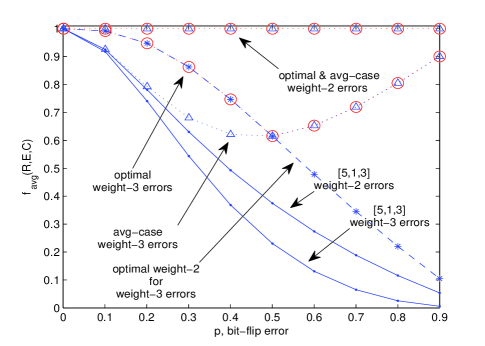
Figure 1: Weight-2 & 3 bit-flip error for the $[5,1,3]$ code, with different recoveries.

Optimized recovery for weight-2,3 bit-flip errors.— Fig. 1 shows $f_{\rm avg}(R,E,C)$ vs. bit-flip probability $p$ with weight-2 and weight-3 errors. In this figure the code is always the standard $[5,1,3]$ code and we compare different recoveries. The solid lines show the $[5,1,3]$ code performance with standard recovery for arbitrary weight-2 or weight-3 errors, which as expected, is not good. The curve with circle markers labeled “optimal weight-3 errors” is for an optimal recovery by solving (23) for the optimal $\gamma$ using the standard $[5,1,3]$ encoding and then finding $R$ from (17)-(22). The improved performance over the solid lines is entirely due to the optimized recovery. Iteration between encoding and recovery [Eqs. (17)-(25)] changed neither the optimized recovery nor the $[5,1,3]$ encoding. We also see that the optimal performance decreases until $p=0.5$ and then increases. The average-case recovery indicated by the dotted curve with triangle markers falls below the optimal for $p<0.5$ and then is identical with the optimal for $p\geq 0.5$. For weight-2 errors, perfect fidelity over the entire $p$-range is achieved by the optimal and average-case recovery (labeled “optimal & avg-case, weight-2 errors”) which are found by solving either (23) for the optimal $\gamma$ or using the approximation (24) and then finding $R$ from (17)-(22). The perfect performance is easily understood from the fact that the $[5,1,3]$ code also perfectly corrects weight-2 bit-flip errors. Our optimization finds the corresponding ideal recovery. When this recovery is applied to the weight-3 errors we get the dashed curve with star markers labeled “optimal weight-2 for weight-3 errors”. This curve follows the weight-3 optimal recovery for $p<0.5$ and diverges thereafter, a phenomenon similar to what was reported for amplitude-damping errors in ReimpellW:05 . In Fig. 1, in all weight-2 cases the recovery matrix $R$ was a $2^{5}\times 2^{5}$ unitary, or easily reducible to that via a singular value decomposition, i.e., no recovery ancillae were needed [recall Eq. (17)]. For weight-3 errors, ${m_{E}}=26$ requires two recovery ancillas, as per Eq. (22) with ${n_{RA}}{n_{CA}}={m_{E}}$.

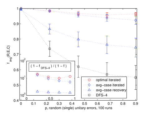
Figure 2: Weight-2 single-random unitary errors for 4-qubit codes.

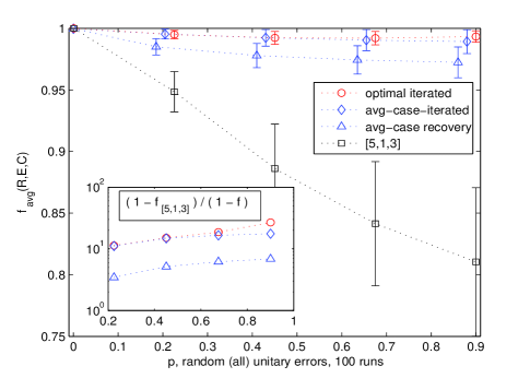
Figure 3: Weight-2 all-random unitary error for 5-qubit codes.

Weight-2 random unitary errors.— Here, with the exception of results marked by “iterated”, we always optimized recovery for the DFS-4 or the $[5,1,3]$ code. In the “iterated” case we start from the DFS-4 or the $[5,1,3]$ code and optimize the encoding as well. We examined two cases: (1) for the DFS-4 code, a single unitary is randomly chosen and used for every one of the 15 errors, thus yielding collective weight-2 errors; (2) for the $[5,1,3]$ code, 15 unitaries are independently randomly selected. While the choice of the DFS-4 code is somewhat arbitrary, we picked this code for case (1) since the errors in this case are similar to the collective decoherence model Zanardi:97c . Figure 2 shows the mean fidelity and standard deviation (error bars) from 100 runs using the DFS-4 code with recovery being the inverse of the encoding (squares), average-case recovery over the whole $p$-range (triangles), iterated average-case (diamonds; encoding optimized as well), and iterated optimal-case recovery at each $p$ (circles). The last two are obtained by iterating (23)-(25) with the $\gamma$-approximation (24) to 5 significant digits. The results for the case when all 15 unitaries are randomly selected are shown in Fig. 3. Here we start from the $[5,1,3]$ code and show standard recovery (squares) vs optimized results (same legend as in Fig. 2). The insets in Figs. 2 and 3 show the fidelity gain relative to recovery via decoding in the DFS-4 case, or relative to standard recovery ($[5,1,3]$ case). In the iterated case, where the encoding is also optimized, the gain is uniformly an order of magnitude or more. It is important to note that this gain is obtained already for small values of $p$, where standard encoding and recovery are designed to perform well. The encoding matrices in the iterated case have support over all basis states and and do not appear to yield previously known codes.

Discussion.— We have presented an optimization approach to quantum error correction that yields codes which achieve robust performance. One way to interpret the results presented in Figs. 1-3 is to consider a scenario where one is faced with a noise channel with weight-2 or 3 errors, and can only use 4 or 5 qubits to encode one. Without optimization perhaps the most reasonable choices are the DFS-4 and [5,1,3] codes. However, our results show that one can obtain at least an order of magnitude higher fidelities by optimizing both the encoding and recovery procedures, while respecting the constraint of 4 or 5 qubits. There are of course standard codes dealing with weight-2 and higher errors, but they require significantly more qubits. We stress again that knowing that such performance is possible can alleviate the need for unnecessary additional codespace which may be impractical, and can help in improving the fault tolerance threshold.

We note that the optimization approaches presented here have differing computational costs. Evaluating this cost depends on the optimization algorithm and the problem structure BoydV:04 . The cost can vary greatly if the algorithm is modified for the specific problem structure. For general comparison purposes, all measures of computational complexity clearly will depend on the dimensions of the various search spaces. This is summarized in Table 1 which gives the number of optimization variables in the SDP optimizations. Clearly, the approximate indirect method enjoys superior scaling.

An intriguing prospect is to integrate the results found here within a complete “black-box” error correction scheme, that takes quantum state or process tomography as input and iterates until it finds an optimal error correcting encoding and recovery. Another important open problem is to extend the robust procedures developed here into a fault-tolerant error correction scheme.

Method		Recovery	Encoding
Direct	Primal (2)	$({n_{S}}^{2}-1){n_{C}}^{2}$	$({n_{C}}^{2}-1){n_{S}}^{2}$
	Dual KosutL:06 ; Fletcher:06	${n_{C}}^{2}$	${n_{S}}^{2}$
Indirect	$\gamma$ opt. (23)	${m_{E}}^{2}=({n_{CA}}{n_{RA}})^{2}$	${n_{S}}{n_{C}}$
	$\gamma$ approx. (24)	0	${n_{S}}{n_{C}}$

Table 1: Number of optimization variables (${n_{C}}={n_{S}}{n_{CA}}$).

Acknowledgments.— Funded under the DARPA QuIST Program and (to D. A. L.) NSF CCF-0523675 and ARO W911NF-05-1-0440. We thank I. Walmsley, D. Browne, C. Brif, M. Grace, and H. Rabitz for enlightening discussions.

References

- (1) P. W. Shor, Phys. Rev. A 52, R2493 (1995); A. M. Steane, Phys. Rev. Lett. 77, 793 (1996); D. Gottesman, Phys. Rev. A 54, 1862 (1996).
- (2) R. Laflamme, C. Miquel, J.P. Paz and W.H. Zurek, Phys. Rev. Lett. 77, 198 (1996).
- (3) E. Knill and R. Laflamme, Phys. Rev. A 55, 900 (1997).
- (4) M.A. Nielsen and I.L. Chuang, Quantum Computation and Quantum Information (Cambridge University Press, Cambridge, UK, 2000).
- (5) M. Reimpell and R. F. Werner, Phys. Rev. Lett. 94, 080501 (2005).
- (6) N. Yamamoto, S. Hara, and K. Tsumara, Phys. Rev. A 71, 022322 (2005); A. S. Fletcher, P. W. Shor, and M. Z. Win, Phys. Rev. A 75, 012338 (2007); M. Reimpell, R.F. Werner, and K. Audenaert, eprint quant-ph/0606059; N. Yamamoto and M. Fazel, eprint quant-ph/0606106.
- (7) R. L. Kosut and D. A. Lidar, eprint quant-ph/0606078.
- (8) S. Boyd and L. Vandenberghe, Convex Optimization (Cambridge University Press, Cambridge, UK, 2004).
- (9) A. Shabani, D.A. Lidar, eprint arXiv:0708.1953.
- (10) D. Kribs and R. Spekkens, Phys. Rev. A 74, 042329 (2006).
- (11) P. Zanardi and D.A. Lidar, Phys. Rev. A 70, 012315 (2004).
- (12) P. Zanardi and M. Rasetti, Phys. Rev. Lett. 79, 3306 (1997).
- (13) A. S. Fletcher, eprint arXiv:0706.3400