Overlapping resonances in the control of intramolecular vibrational redistribution

Abstract

Coherent control of bound state processes via the interfering overlapping resonances scenario [Christopher et al., J. Chem. Phys. 123, 064313 (2006)] is developed to control intramolecular vibrational redistribution (IVR). The approach is applied to the flow of population between bonds in a model of chaotic OCS vibrational dynamics, showing the ability to significantly alter the extent and rate of IVR by varying quantum interference contributions.

I Introduction

Quantum control of molecular processesbook1 ; book has proved, over the past two decades, to be viable both theoretically and experimentally. An examination of the coherent control literature, wherein scenarios are expressly designed to take advantage of quantum interference phenomena, shows that the vast majority of applications has been to processes occurring in the continuum energy regime. Recently we proposed a new approach to controlling bound state dynamics in large polyatomic moleculescsb that exploits interferences between overlapping resonances. We have demonstrated the viability of this scenario in controlling internal conversion in pyrazine.csb ; csb2 ; csb3 In the present paper we further develop this method, applying it to the control of Intramolecular Vibrational Redistribution (IVR). As an example, we study the control of the flow of energy between bonds in a model of OCS. This molecule, though small, is of particular interest at high energies, where, classically, it displays predominantly chaotic dynamics. In spite of the classical chaos, quantum control via the present scenario is shown to be excellent.

This paper is organized as follows: Section II provides an overview of the theory, with a discussion of the Feshbach partitioning technique which, as we have shown,csb provides a highly efficient method for dealing with bound state problems. Section III describes the collinear OCS model and its classical dynamical characteristics. In Section IV we discuss the application of the method to the control of IVR in OCS. An Appendix describes our use of the Feshbach partitioning technique for the numerical solution of the bound state problem for small systems such as OCS. A more ambitious method for addressing considerably larger systems, the “QP algorithm”, is described elsewhere.csb2

II Bound State Control

II.1 Time-evolution of populations in molecular systems

We consider a system described by an Hamiltonian $H$ which can be partitioned physically into the sum of two components $H_{A}$ and $H_{B}$, plus the interaction $H_{AB}$ between them:

$$H=H_{A}+H_{B}+H_{AB},$$ (1)

The eigenstates and eigenvalues of the full Hamiltonian are defined by:

$$H|{\gamma}\rangle=E_{\gamma}|{\gamma}\rangle~{}.$$ (2)

The (“zeroth-order”) eigenstates and eigenvalues of the sum of the decoupled Hamiltonians are defined as

$$(H_{A}+H_{B})|\kappa\rangle=E^{(\kappa)}|\kappa\rangle~{}.$$ (3)

Below, we are interested in the time evolution of the system, initially prepared in a superposition of zeroth order states.

$$|\Psi(t=0)\rangle=\sum_{\kappa}c_{\kappa}|\kappa\rangle,$$ (4)

where $\{c_{\kappa}\}$ are “preparation” coefficients. All sums over $|{\kappa}\rangle$, here and below, are assumed to be confined to a subspace $S$. For example, the selected initial states might consist of a set with population heavily concentrated in one bond of a molecule, in which case, energy flow out of such superposition states is examined.

The time-evolution of Eq. (4) at any subsequent time can then be obtained by expanding the (zeroth order) eigenstates, $|\kappa\rangle$, in terms of the exact eigenstates $|{\gamma}\rangle$ to give:

$$|{\Psi(t)}\rangle=\sum_{\kappa,\gamma}c_{\kappa}a_{\kappa,\gamma}^{*}e^{-iE_{\gamma}t/\hbar}|{\gamma}\rangle,$$ (5)

with $a_{\kappa,\gamma}^{*}=\langle{\gamma}|{\kappa}\rangle$. The structure of $|\langle{\gamma}|{\kappa}\rangle|^{2}$ as a function of $\gamma$ defines a resonance shape that provides insight, in the frequency domain, into the population flow out and into the zeroth order $|{\kappa}\rangle$ states.

Given this time evolution, the amplitude for finding the system in a state $|{\kappa}\rangle$ at time $t$ is

$$c_{\kappa}=\langle{\kappa}|{\Psi(t)}\rangle=\sum_{\kappa^{\prime}}c_{\kappa^{\prime}}M_{\kappa,\kappa^{\prime}}(t),$$ (6)

where

$$M_{\kappa,\kappa^{\prime}}(t) \equiv \sum_{\gamma}a_{\kappa,\gamma}a_{\kappa^{\prime},\gamma}^{*}e^{-iE_{\gamma}t/\hbar}$$ (7)

$$= \langle{\kappa}|\left(\sum_{\gamma}e^{-iE_{\gamma}t/\hbar}|{\gamma}\rangle\langle{\gamma}|\right)|{\kappa^{\prime}}\rangle$$

is the ($\kappa,\kappa^{\prime}$) element of the overlap matrix ${\bf M}(t)$ defined by the term in brackets in Eq. (7). Note that, for $\kappa^{\prime}\neq\kappa$, if the states $|{\kappa}\rangle$ and $|{\kappa^{\prime}}\rangle$ do not overlap with a common $|{\gamma}\rangle$, i.e., there are no overlapping resonances, then $M_{\kappa,\kappa^{\prime}}=0$. Our previous studiescsb have demonstrated the significance of such overlapping resonances to the control of radiationless transitions, such as internal conversion.

From Eq. (6), the probability of finding the system in a collection of states $|{\kappa}\rangle$ contained in the initial set $S$ at time $t$ is given by

$$P(t)=\sum_{\kappa}|\langle{\kappa}|{\Psi(t)}\rangle|^{2}={\bf c}^{\dagger}{\bf K}(t){\bf c},$$ (8)

where ${\bf c}$ is a $\kappa$-dimensional vector whose components are the $c_{\kappa}$ coefficients, and ${\bf K}(t)\equiv{\bf M}^{\dagger}(t){\bf M}(t)$. The generalization to the question of finding population in an alternative collection of states, other than $S$, is straightforward. However, it is unnecessary for the study below, as will become evident. Equation (8) allows us to address the question of enhancing or restricting the flow of probability out of $S$ by finding the optimal combination of $c_{\kappa}$ that achieves this goal at a specified time $T$. Experimentally, the resultant required superposition state can be prepared using modern pulse shaping techniques.

II.2 The Feshbach partitioning technique

Our interest is to control the flow of population out of some generic molecular subspace into the entire molecular Hilbert space. In order to do so we make use of the bound state version of the Feshbach partitioning technique.f ; Levine Here, since the control approach is being tested on a small system, we solve the resulting equations in a straightforward way, as described in Appendix A. Larger systems can take advantage of the “QP algorithm”.csb2

The Feshbach partitioning technique is based on defining two projection operators

$$Q\equiv\sum_{\kappa}|{\kappa}\rangle\langle{\kappa}|,\quad P\equiv\sum_{\beta}|{\beta}\rangle\langle{\beta}|,$$ (9)

which satisfy the following properties:

$$Q^{2}=Q,\quad P^{2}=P,$$ (10a)

$$[Q,P]=0,$$ (10b)

$$P+Q=\mathbb{I},$$ (10c)

where $\mathbb{I}$ is the identity operator. In what follows, the flow of probability of interest is from the $Q$ space to the $P$ space.

Using Eqs. (10c) and (9), the eigenstates of the full Hamiltonian can be written as

$$|{\gamma}\rangle=\sum_{\kappa}|{\kappa}\rangle\langle{\kappa}|{\gamma}\rangle+\sum_{\beta}|{\beta}\rangle\langle{\beta}|{\gamma}\rangle.$$ (11)

Similarly, the Schrödinger equation can be expressed as

$$[E_{\gamma}-H][P+Q]|{\gamma}\rangle=0,$$ (12)

whereby multiplying it by $P$ and then by $Q$, and using Eq. (10), one obtains the following set of coupled equations:

$$\left[E_{\gamma}-PHP\right]P|{\gamma}\rangle = PHQ|{\gamma}\rangle,$$ (13a)

$$\left[E_{\gamma}-QHQ\right]Q|{\gamma}\rangle = QHP|{\gamma}\rangle.$$ (13b)

The states $|{\kappa}\rangle$ and $|{\beta}\rangle$ are solutions to the decoupled (homogeneous) equations arising from Eqs. (13a) and (13b), respectively. That is,

$$\left[E_{\beta}-PHP\right]P|{\beta}\rangle=0,$$ (14a)

$$\left[E_{\kappa}-QHQ\right]Q|{\kappa}\rangle=0.$$ (14b)

Contrary to continuum problems, in general $E_{\gamma}\neq E_{\beta}$ and it is possible to express $P|{\gamma}\rangle$ in terms of the particular solution of the (inhomogeneous) Eq. (13a),

$$P|{\gamma}\rangle=[E_{\gamma}-PHP]^{-1}PHQ|{\gamma}\rangle.$$ (15)

Substituting Eq. (15) into Eq. (13b) results in

$$[E_{\gamma}-QHQ]Q|{\psi}\rangle=QHP[E_{\gamma}-PHP]^{-1}PHQ|{\psi}\rangle.$$ (16)

By rearranging terms in this equation, one obtains

$$[E_{\gamma}-{\cal H}]Q|{\gamma}\rangle=0,$$ (17)

where ${\cal H}$ is an effective Hamiltonian, defined as

$${\cal H}=QHQ+QHP[E_{\gamma}-PHP]^{-1}PHQ.$$ (18)

The term between squared brackets can be written as

$$\left[E_{\gamma}-PHP\right]^{-1}=\sum_{\beta}\frac{1}{E_{\gamma}-E_{\beta}}|{\beta}\rangle\langle{\beta}|$$ (19)

by using the spectral resolution of an operator. The matrix elements of ${\cal H}$ are given by

$$\langle{\kappa}|{{\cal H}}|{\kappa^{\prime}}\rangle=E_{\kappa}\delta_{\kappa,\kappa^{\prime}}+\Delta_{\kappa,\kappa^{\prime}},$$ (20)

where

$$\Delta_{\kappa,\kappa^{\prime}}=\frac{1}{2\pi}\sum_{\beta}\frac{\Gamma_{\kappa,\kappa^{\prime}}}{{E_{\gamma}-E_{\beta}}},$$ (21a)

$$\Gamma_{\kappa,\kappa^{\prime}}=2\pi V(\kappa|\beta)V(\beta|\kappa^{\prime}),$$ (21b)

with $V(\kappa|\beta)=\langle{\kappa}|{QHP}|{\beta}\rangle$ being the coupling term. Equations (21a) and (21b) represent the energy shift and the decay rate, respectively. By diagonalizing Eq. (17) in a self-consistent manner, one obtains the energy eigenvalues, $E_{\gamma}$, and the values for the overlap integrals, $a_{\kappa,\gamma}$.

$i$		$D_{i}$		$\beta_{i}$		$R_{i}^{0}$
1		0.08518		1.5000		2.9759
2		0.21238		1.6251		2.2559
3		0.16000		1.1589		2.8037

Table 1: Parameters defining the potential energy surface given by Eq. (32). All magnitudes are given in a.u.

Note that the energy eigenvalues and the overlap integrals can also be obtainedthesis by directly diagonalizing the full Schrödinger equation in the zeroth-order basis. However, the partitioning technique presented above has computational advantages for cases where the dimensions of the $P$ space is large, since one only needs to diagonalize an effective Hamiltonian ${\cal H}$ with dimensions given by the $Q$ space. Note, however, that diagonalizing ${\cal H}$ requires using iterative procedures, and needs to be solved repeatedly until each eigenvalue is found. Appendix A provides details on the partitioning algorithm used here.

II.3 Optimal Control

To determine the set of optimal preparation coefficients leading to either a maximum or a minimum population at time $t=T$, we need to find the extrema of the functionfs

$$P_{\lambda}(t)={\bf c}^{\dagger}{\bf K}(t){\bf c}-\lambda{\bf c}^{\dagger}{\bf c}$$ (22)

with respect to the coefficients ${\bf c}$, where $\lambda$ is a Lagrange multiplier added to assure normalization, i.e.,

$$\sum_{\kappa}|c_{\kappa}|^{2}=1.$$ (23)

The optimum vector, ${\bf c}_{T}$, is obtained by differentiating Eq. (22) with respect to the components of ${\bf c}^{\dagger}$, and equating the resulting expression to zero at time $T$, i.e.,

$$\frac{\partial P_{\lambda}(t)}{\partial c_{\kappa^{\prime}}^{*}}\bigg{|}_{t=T}=\sum_{\kappa}{\bf K}_{\kappa^{\prime},\kappa}(T)c_{\kappa}-\lambda c_{\kappa}=0.$$ (24)

The optimum vector resulting from this procedure is a solution to the eigenvalue problem represented by Eq. (24). Note that this vector can either maximize or minimize the solution. In the first case, the interference between overlapping resonances created by the initial superposition will be seen to result in a delay of the population decay, whereas in the second case the population decay is being accelerated.

In order to further clarify the dependence of the time-evolution on overlapping resonances, Eq. (8) can be re-expressed as

$$P(t)=\sum_{\kappa}|c_{\kappa}|^{2}g_{\kappa}+\sum_{\begin{subarray}{c}\kappa^{\prime},\kappa\\ \kappa^{\prime}\neq\kappa\end{subarray}}c_{\kappa^{\prime}}^{*}c_{\kappa}f_{\kappa^{\prime},\kappa},$$ (25)

where

$$g_{\kappa}=\sum_{\kappa^{\prime}}|M_{\kappa^{\prime},\kappa}|^{2},$$ (26)

and

$$f_{\kappa^{\prime},\kappa}=\sum_{\kappa^{\prime\prime}}M^{*}_{\kappa^{\prime\prime},\kappa^{\prime}}M_{\kappa^{\prime\prime},\kappa}.$$ (27)

As expressed in Eq. (25), the $Q$ space population assumes the generic coherent control formbook ; book1 : it is given as the sum of non-interfering pathways, represented by $g_{\kappa^{\prime}}$, and interfering pathways, represented by $f_{\kappa^{\prime},\kappa}$.

II.4 The Role of Overlapping Resonances

The interference term in Eq. (25) depends on $f_{\kappa^{\prime},\kappa}$, which, in accord with Eq. (27), depends upon the overlap between resonances. Qualitatively speaking, a resonance is described by bound states $|{\kappa}\rangle$ coupled to a quasi-continuum of exact eigenstates $|{\gamma}\rangle$. Each such state is thus associated with the energy width of the $\langle\kappa|\gamma\rangle$ overlap coefficients. Overlapping resonances are the result of having at least two states whose resonance widths are wider than their associated level spacing. The resulting resonances interfere with one another, displaying a variety of lineshapes,book and are responsible for the interference in this control scenario. In the absence of overlapping resonances the full $f_{\kappa^{\prime},\kappa}$-term in Eq. (25) vanishes and control disappears.

Note that there are also contributions from overlapping resonances to the $g_{\kappa}$-term, as can be seen from their effect on the nature of the decay from the individual $|{\kappa}\rangle$. These resonances distort the lineshape, and hence the corresponding time dependence. In order to determine the contribution from overlapping resonances, we have devisedcsb a qualitative measure, defined as

$$\tilde{P}(t)=[P(t)-W(t)],$$ (28)

where

$$W(t)=\sum_{\kappa}|c_{\kappa}M_{\kappa,\kappa}|^{2}.$$ (29)

Here $W(t)$ is a measure of the direct contribution, and $\tilde{P}(t)$ provides a measure of the overlapping resonance contribution. In the absence of overlapping resonances, $P(t)=W(t)$.

III Classical aspects of the collinear OCS

III.1 The OCS model

As a working model to illustrate the usefulness of the method described in Sec. II, we consider a collinear model of OCS, with a modified Sorbie-Murrellcb potential. The interest in this system arises from the fact that, close to dissociation, i.e. in the energy region of interest below, the classical dynamics becomes highly chaotic. As such, collinear OCS is a complex system with a penchant for extensive IVR.

The classical dynamics of OCS has been studied in both planar,cb and collinear Davis1 ; Davis2 versions. Here, we consider the collinear case, which is described by the Hamiltonian

$$H=\frac{P_{1}^{2}}{2\mu_{13}}+\frac{P_{2}^{2}}{2\mu_{23}}-\frac{P_{1}P_{2}}{m_{C}}+V(R_{1},R_{2},R_{3}),$$ (30)

where

$$\mu_{13} = \frac{m_{O}m_{C}}{m_{O}+m_{C}}$$

$$\mu_{23} = \frac{m_{S}m_{C}}{m_{S}+m_{C}},$$ (31)

are reduced masses; $R_{1}$ and $R_{2}$ are the CS and CO bond distances, respectively ($R_{3}=R_{1}+R_{2}$); and $P_{1}$ and $P_{2}$ are the corresponding momenta.

In the course of this work we found that the Sorbie-Murrell OCS modelcb displayed a second minimum at large distances along both the CS and CO exit channels. Although the depth of this second well is extremely small, there are a large number of closely packed eigenstates localized in this region due to the length of the well. To our knowledge, there is no experimental evidence to either support or refute a second minimum, although they have been associatedozone with van der Waals interactions in O₃. However, in order to ensure that the observed control is not a manifestation of this secondary minimum (as was the case in our preliminary studies) a modified interaction potential is used that removes these second minima while retaining the general features of the remaining potential. Specifically, the potential used here consists of a sum of three Morse functions,

$$V(R_{1},R_{2},R_{3})\equiv\sum_{i=1}^{3}V_{i}=\sum_{i=1}^{3}D_{i}\left[1-e^{-\beta_{i}(R_{i}-R_{i}^{0})}\right]^{2},$$ (32)

with parameters given in Table 1. A contour plot of the resultant potential energy surface is shown in Fig. 1. Except for the Morse function $V_{3}$, which depends on $R_{3}$, the parameters defining the other two Morse functions have been changed so that the potential smoothly fits the original one along the equilibrium directions while, at the same time, eliminating the second potential minima. Moreover, we have also modified the added constant in the potential so that the CS dissociation onset [$V(\infty,R_{2}^{0})=D_{1}+D_{3}$] corresponds to the original value of $E_{d}=0.100$ a.u.

Figure 1: Contour plot of the potential energy surface given by Eq. (32). Solid and dashed lines represent, respectively, energy contours above and below the dissociation onset, at $E=0.100$ a.u. (thick solid line).

III.2 Characterizing the Dynamics

The classical dynamics of the resultant OCS model is characterized by a smooth transition from regular to chaotic dynamics with increasing energy. At an energy just below dissociation, ($E_{0}=0.09796$4 a.u., of interest below), the Poincare surface of sectionPSOS shows [Fig. 2(a)] highly chaotic dynamics, with a stable region constituting about $1/3$ of the phase-space portrait. This energy corresponds to the mean value of the energies of the two wave packets, $|\Psi_{\pm}\rangle$, obtained below in maximizing and minimizing the energy flow from the CS bond. Surfaces of section in the nearby energies are essentially similar. This being the case, there is no obvious classical origin to the control of bond energy relaxation described below. Of some future interest, however, might be an auxiliary study of the relationship of overlapping resonances induced control, observed below, to classical features such as bond energy recurrences, cantori, and the inhomogeneous character of the OCS phase space Eckhardt1 ; Davis1 ; Davis2 ; Chirikov ; Wyatt ; Davis3 .

Figure 2: (a) Poincaré surface of section for the collinear OCS model at $E=0.09796$ a.u. The solid line represents the total energy contour. (b) Distance between two nearby trajectories (with $d_{0}=10^{-8}$ a.u.) chosen in the stable region ($\blacktriangledown$), and in the chaotic sea ($\blacktriangle$). The high-frequency oscillations have been averaged out in both cases (the smoothing causes $\Lambda^{(\blacktriangledown)}$ to appear as if it does not begin at zero). (c) CS–bond vibrational energy corresponding to the chaotic trajectory of part (b).

Quantitative insight into the rate of loss of correlations in the chaotic region of phase space can be obtained by computing Lyapunov exponents,Lieberman approximated by the average (over various trajectories) of the exponential rate at which the distance $d(t)$ between adjacent trajectories in phase space grow in time:

$$\lambda_{\infty}=\lim_{t\to\infty}\frac{1}{t}\ln\frac{d(t)}{d_{0}}.$$ (33)

Here, in order to show how different regular and chaotic trajectories behave, we have computed the quantity

$$\Lambda(t)=\ln\frac{d(t)}{d_{0}},$$ (34)

with $d_{0}=10^{-8}$ a.u. We label the finite time Lyapunov exponent, computed in this way, as $\lambda_{t}$.

The quantity $\Lambda(t)$ is shown in Fig. 2(b) for two sets of nearby trajectories,note2 picked in two different regions of phase-space: the stable island, and the chaotic sea. The results, to $t\approx 1.2$ ps, give $\lambda_{t}^{(stable)}\simeq 1.46$ ps^-1, and $\lambda_{t}^{(chaotic)}\simeq 17.41$ ps^-1 in the regular and chaotic regions, respectively. The associated times are to be compared to zeroth order vibrational periods (27.45 fs for the CS bond, and 18.10 fs for the CO bond).

Finally, in Fig. 2(c) we show the energy in the CS bond, for a trajectory in the chaotic sea. As can be seen, the energy displays a complicated pattern, with irregular energy transfer between both bonds as a function of time. Nonetheless, when one computes the energy average of an ensemble of trajectories, the pattern becomes smooth and displaying a profile than can be fitted to an exponential decay,Davis2 similar to those observed in its quantum counterpart below.

IV Coherent control of IVR

IV.1 Population decay

				IVR suppression								IVR enhancement
$\kappa$		$E_{\kappa}$ (a.u.)			$c_{\kappa}^{r}$			$c_{\kappa}^{i}$		$|c_{\kappa}|^{2}$			$c_{\kappa}^{r}$			$c_{\kappa}^{i}$		$|c_{\kappa}|^{2}$		$t_{\delta}$ (fs)
1		0.0851446			0.02895			0.00000		0.00084		$-$​	0.13839			0.00000		0.01915		17.84
2		0.0850268		$-$​	0.00706			0.17289		0.02994			0.38027		$-$​	0.00806		0.14467		8.03
3		0.0848265			0.16188		$-$​	0.16611		0.05380		$-$​	0.00128		$-$​	0.10472		0.01097		16.25
4		0.0845437		$-$​	0.56608			0.25828		0.38716			0.01257		$-$​	0.08349		0.00713		20.76
5		0.0841783			0.18017		$-$​	0.24251		0.09127		$-$​	0.03560			0.05674		0.00449		13.69
6		0.0837303			0.20267			0.15178		0.06411			0.19804			0.05108		0.04183		34.02
7		0.0831998		$-$​	0.21171			0.16534		0.07216			0.12120		$-$​	0.63185		0.41392		20.53
8		0.0825867			0.25004		$-$​	0.41477		0.23455			0.20859		$-$​	0.39177		0.19699		25.32
9		0.0818910		$-$​	0.05482			0.25131		0.06616			0.24895		$-$​	0.31440		0.16082		22.95

Table 2: Values corresponding to the eigenstates for the (uncoupled) CS bond used in the optimized superpositions. $E_{\kappa}$ denotes the energy associated to these eigenstates; $c_{\kappa}^{r}$ and $c_{\kappa}^{i}$ are the real and imaginary parts of the $c_{\kappa}$ coefficients, respectively; and $t_{\delta}$ is the decay time (see text for details). The optimization to maximize/minimize the energy transfer into the CO bond (suppression/enhancement of IVR) has been carried out at $T=100$ fs. The energy corresponding to the ground state in the (uncoupled) CO bond is $E_{CO}^{0}=0.00360475$ a.u.

We now consider the suppression (and enhancement) of IVR in the above model of OCS. Our intent is to assess the extent of control in such a system, and to establish the relationship between control and overlapping resonances. The coupling terms $V(\kappa|\beta)$ and, subsequently, the overlap integrals $a_{\kappa,\gamma}$ and the energy eigenvalues $E_{\gamma}$ are calculated by expanding the OCS wave functions in products of the zeroth order states,

$$|{\Psi}\rangle=\sum_{m,n}|{\eta_{CS}^{m}}\rangle\otimes|{\xi_{CO}^{n}}\rangle d_{mn}~{}.$$ (35)

where $|{\eta_{CS}^{m}}\rangle$ and $|{\xi_{CO}^{n}}\rangle$ are eigenstates of the uncoupled CS and CO bond potentials, respectively, with quantum numbers $m$ and $n$. Our interest is in the flow, for example, out of the CS bond. Hence, the $Q$ subspace is chosen to represent all wave functions containing only excitation in the CS bond, i.e., $|{\kappa}\rangle$ are $|{\eta_{CS}^{m}}\rangle\otimes|{\xi_{CO}^{0}}\rangle$, for all $m$, whereas the $P$ subspace spans the space represented by all other zeroth order excitations, i.e., the $|{\beta}\rangle$ are $|{\eta_{CS}^{m}}\rangle\otimes|{\xi_{CO}^{n}}\rangle,n\neq 0$, describing excitation in the CS bond. Initiating excitation within $Q$ and watching the flow into $P$ then corresponds to an experiment wherein excitation flows out of the CS bond.

As seen in Sec. III.1, the coupling term, $QHP$, necessary to obtain the energy shifts and decay rates, consists of a static term ($V_{3}$), and a dynamic term [proportional to $p_{1}p_{2}$ in Eq. (30)]. The overlap integrals and energy eigenvalues are obtained by self-consistent diagonalization of Eq. (17). All vibrational states, $|{\eta_{CS}^{m}}\rangle$ and $|{\xi_{CO}^{n}}\rangle$, are numerically calculated using a discrete variable representation (DVR) technique,Light obtaining a total of 45 eigenvectors for the CS bond, and 59 for the CO bond. The number of eigenvectors is larger in the second case, because the dissociation threshold of the CO bond is higher in energy.

From all the vibrational states obtained, we have observed that control is best when considering a superposition of states, i.e., Eq. (4), that is near the dissociation onset. The energy differences between these states are relatively small ($\approx 0.0004$ a.u., whose inverse corresponds to a timescale of $\approx 60$ fs), thus giving rise to a high density of states with time scales comparable to vibrational relaxation. The result is a greater opportunity for overlapping resonances which, as will be seen below, enhances the ability to control energy flow. In our case, the states used are the last nine bound eigenvectors (before the dissociation onset) of the CS bond, whose corresponding eigenvalues are given in Table 2. Note, however, that dense eigenstate manifolds will occur at far lower energies in larger molecules. Hence, the initial $|{\Phi(0)}\rangle$ is comprised of a superposition of nine CS states in Table 1, with the CO in the ground vibrational state.

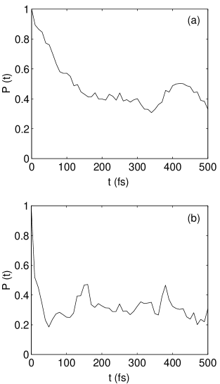
Figure 3: IVR control in OCS: (a) IVR suppression, and (b) IVR enhancement. The parameters defining the optimal superposition for $T=100$ fs are given in Table 2.

Figure 4: Individual decay for wave functions consisting of each individual eigenvector used in the construction of the optimal superpositions. The labels correspond to those given in Table 2.

Figure 3 shows the time-evolution of the population, $P(t)$, for an initial wave function constructed from the nine zeroth order $Q$ space states noted above, and optimized for maximal or minimal energy flow at $T=100$ fs. The optimal coefficients were found using the method described in Sec. II; the $c_{\kappa}$ coefficients and their probabilities are given in Table 2. Results in panel (a) correspond to an initial superposition optimized to minimize the population flow from the $Q$ to the $P$ space, while panel (b) shows results optimized to enhance the flow of population. As is clearly seen, the initial falloff in panel (a) is much slower than that in (b). To quantify this decay, the initial $P(t)$ falloff was fit to an exponentially decreasing function,

$$P(t)=P_{\infty}+(1-P_{\infty})e^{-t/t_{\delta}},$$ (36)

where $t_{\delta}$ is the decay time, and $P_{\infty}$ is the average around which $P(t)$ fluctuates for the first 1.0 ps. Note that the $t_{\delta}$ values can only be regarded as approximate since the falloff is, in general, not exponential, and $t_{\delta}$ depends on the time scale over which the exponential is fit. (Here the fit is over 400 fs). In case (a), the decay time is $t_{\delta}\simeq 57.35$ fs, while in case (b) it is $t_{\delta}\simeq 8.60$ fs, about seven times smaller. Furthermore, we note that in panel (a), only about $24$% of the population has been transferred from $Q$ to $P$ during the first 50 fs, while, in contrast, approximately 82% of the population has being transferred to the $P$ in panel (b) during the same time. Moreover, the population that asymptotically remains localized along the CS bond is also larger in the case of IVR suppression ($P_{\infty}\simeq 0.4$) than in that of enhancement ($P_{\infty}\simeq 0.3$).

The controlled results should be compared to the natural IVR behavior of the individual levels participating in the superposition. To this end, the $P(t)$ for each of the participating levels is shown in Fig. 4. Although the energy difference between these states shown is relatively small, the populations, $P_{\kappa}$, evolve with a range of initial falloff values, as can be seen in the corresponding values of $t_{\delta}$, given in Table 2. Note also, from this table, that the control seen in Fig. 3 is not due to the identification of a particular $|\kappa\rangle$ that independently maximizes or minimizes the decay. Indeed, by inspecting the value of the $c_{\kappa}$ coefficients, we find, in the case of IVR suppression, participation of most of the nine levels, with $\approx$ 60% of the total initial population concentrated in the two states with $\kappa=4$ and $\kappa=8$. Neither of these two states independently have the longest decay times, but their interference is crucial to control. Similar observations result from considering the data for optimized IVR enhancement, despite the fact that $\kappa=2$ has a relatively small $t_{\delta}$. In this case the optimized superposition also gives a significantly smaller $P(T)$ than does the individual $\kappa=2$ state.

A qualitative measure $\tilde{P}(t)$ of the contribution from the interference of overlapping resonances, and $W(t)$ from the direct contribution, was provided in Eq. (28). Results for $\tilde{P}(t)$ and $W(t)$ for the maximization and minimization cases above are provided in Fig. 5 where the contribution from overlapping resonances (dashed line), become dominant after the first 10 fs, thus demonstrating the important role played by these resonances in the IVR control scenario. This is seen to be the case for both the maximization, as well as minimization, of the flow from the CS bond.

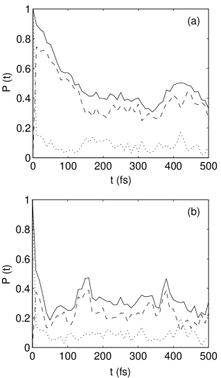
Figure 5: Contribution of $\tilde{P}(t)$ (dashed line) and $W(t)$ (dotted line) to: (a) IVR suppression, and (b) IVR enhancement. The solid line represents the corresponding $P(t)$ function from Figs. 3.

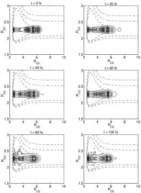
Figure 6: Wave packet evolution corresponding to IVR suppression. Dashed lines represent equipotential energy contours, with the innermost corresponding to the wave packet energy, $E_{+}=0.09849$ a.u.

A pictorial, and enlightening, view of the results is provided in Figs. 6 and 7, where the wave packets associated with IVR suppression and enhancement are shown. As can be seen in Fig. 6, for the case of IVR suppression, the wave packet remains highly localized along the $R_{\rm CS}$ mode, with minimum spreading along the $R_{\rm CO}$ mode. In particular, it undergoes a slight oscillation along the $R_{\rm CS}$ mode, concentrating most of the probability around the region where the CS dissociation takes place, in a clear correspondence to what happens with a classical counterpart. For the case of IVR enhancement, the effect is the opposite. As can be seen in Fig. 7, the spreading of the wave packet along the $R_{\rm CO}$ mode coordinate is relatively fast.

The method described above is, of course, applicable at any time during the dynamics. For example, we tried, and successfully attained, control for times at long as 1.5 ps (corresponding to over 50 CS vibrational periods), resulting in about a 55% of the population localized in the CS bond for IVR suppression, and about 22% for IVR enhancement.

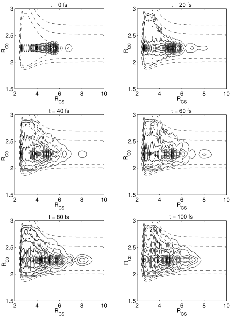
Figure 7: Wave packet evolution corresponding to IVR enhancement. Dashed lines represent equipotential energy contours, with the innermost corresponding to the wave packet energy, $E_{-}=0.09743$ a.u.

V Comments and Summary

In this paper, a method for controlling intramolecular vibrational redistribution has been developed and has been applied to OCS, where extensive control over IVR is attained. Of particular interest is that the control is achieved even though the associated classical dynamics is chaotic. The method, wherein the coefficients of an initial superposition of zeroth order states are optimized, is shown to rely upon the presence of overlapping resonances, a feature which is expected to be ubiquitous in realistic molecular systems.

We have assumed throughout this paper that the initial state that optimizes the intramolecular vibrational redistribution can be prepared, for a real molecule, using modern pulse shaping techniques. Computations displaying the resultant field were not, however, carried out on this OCS model since they are best done using more realistic molecular potentials in higher dimensions, yielding realistic optimizing fields. Work of this kind is in progress.

Appendix A Numerical Implementation

Here, we provide a route to compute the eigenvalues and overlap integrals via Eq. (17). We start by defining $N_{\kappa}$ and $N_{\beta}$ to be the basis-set dimensions in the $Q$ and $P$ space, respectively, and $N_{T}=N_{\kappa}+N_{\beta}$. The probability of being in the $Q$ space, $P(t)$, is given by Eq. (8). In order to find $P(t)$, two sets of values are needed: the set of eigenvalues $\{E_{\gamma}\}$, and the overlap integrals $a_{\kappa,\gamma}$ between the zeroth-order states in $Q$ and the exact eigenstates $|{\gamma}\rangle$. The partitioning algorithm described below is ingenious in the sense that it allows one to concentrate specifically on obtaining these two sets of values. The method is well suited to small systems.

Beginning with Eq. (17), and using Eqs. (21), the algorithm is as follows:

1. Choose a starting energy $E_{\gamma}^{i=0}$, with $i$ corresponding to the $i$th iteration. In particular, one may choose an energy close to the zeroth-order energies.

2. Take $E_{\gamma}^{i}$ from the last iteration, and compute ${\cal H}(E_{\gamma}^{i})$.

3. Diagonalize ${\cal H}(E_{\gamma}^{i})$, and select one of its eigenvalues to be the next trial energy, $E_{\gamma}^{i+1}$.

4. If $|E_{\gamma}^{i+1}-E_{\gamma}^{i}|\ncong 0$, go back to step 2.

5. If $|E_{\gamma}^{i+1}-E_{\gamma}^{i}|\cong 0$, $E_{\gamma}^{i+1}$ becomes the eigenvalues $E_{\gamma}$, and its corresponding eigenvector, $|{D_{\gamma}}\rangle$, is proportional to $Q|{\gamma}\rangle$.

6. Repeat steps 1-5 until all $N_{T}$ unique eigenvalues $E_{\gamma}$ are obtained.

In the process of diagonalizing the effective Hamiltonian, ${\cal H}$, each eigenvector $|{D_{\gamma}}\rangle$ has been normalized to 1. Therefore, the use of the algorithm leads to a loss of information about $Q|{\gamma}\rangle$. This makes necessary to also compute the constant of proportionality between $Q|{\gamma}\rangle$ and $|{D_{\gamma}}\rangle$. This is done by requiring that $\langle{\gamma}|{\gamma}\rangle=1$ for the full eigenvectors. Thus, one can assert that

$$Q|{\gamma}\rangle=C_{\gamma}|{D_{\gamma}}\rangle,$$ (37)

with $C_{\gamma}$ being the proportionality constant. The problem then reduces to finding the $C_{\gamma}$ associated with each $E_{\gamma}$. This is accomplished by expressing $\langle{\gamma}|{\gamma}\rangle$ as

$$\langle{\gamma}|{\gamma}\rangle = \langle{\gamma}|{Q}|{\gamma}\rangle+\langle{\gamma}|{P}|{\gamma}\rangle$$ (38)

$$= \langle{\gamma}|{Q^{2}}|{\gamma}\rangle+\langle{\gamma}|{P^{2}}|{\gamma}\rangle,$$

where

$$\langle{\gamma}|{Q^{2}}|{\gamma}\rangle=|C_{\gamma}|^{2}\langle{D_{\gamma}}|{D_{\gamma}}\rangle=|C_{\gamma}|^{2},$$ (39)

and, using Eq. (15),

$$\langle{\gamma}|{P^{2}}|{\gamma}\rangle = \langle\gamma|QHP\left[E_{\gamma}-PHP\right]^{-1}$$ (40)

$$\times \left[E_{\gamma}-PHP\right]^{-1}PHQ|\gamma\rangle.$$

The application of the spectral resolution of an operator, Eq. (19), to Eq. (40) leads to

$$\langle\gamma|P^{2}|\gamma\rangle=\sum_{\beta}\frac{\langle\gamma|QH|\beta\rangle\langle\beta|HQ|\gamma\rangle}{\left(E_{\gamma}-\widehat{E}_{\beta}\right)^{2}},$$ (41)

whereby, by making use of Eq. (37), one obtains

$$\langle\gamma|P^{2}|\gamma\rangle=\left|C_{\gamma}\right|^{2}\sum_{\beta}\frac{\langle D_{\gamma}|H|\beta\rangle\langle\beta|H|D_{\gamma}\rangle}{\left(E_{\gamma}-\widehat{E}_{\beta}\right)^{2}}.$$ (42)

Now $\langle\gamma|P^{2}|\gamma\rangle$ is easily computed by realizing that

$$\langle D_{\gamma}|H|\beta\rangle = \sum_{\kappa}D_{\kappa\gamma}^{*}\langle\kappa|H|\beta\rangle$$ (43)

$$= \sum_{\kappa}D_{\kappa\gamma}^{*}V(\kappa|\beta).$$ (44)

The substitution of Eqs. (39) and (42) into Eq. (38) yields

$$\langle\gamma|\gamma\rangle=1=\left|C_{\gamma}\right|^{2}\left(1+\sum_{\beta}\frac{\left|\sum_{\kappa}D_{\kappa\gamma}^{*}V(\kappa|\beta)\right|^{2}}{\left(E_{\gamma}-\widehat{E}_{\beta}\right)^{2}}\right),$$ (45)

from which one obtains the proportionality factor $|C_{\gamma}|$.

According to the procedure previously described, we can determine $Q|\gamma\rangle$, given $|D_{\gamma}\rangle$, with the exception of a constant phase factor. Note that, in general, each proportionality factor, $C_{\gamma}$, can be written as $|C_{\gamma}|e^{\theta_{\gamma}}$, where $\theta_{\gamma}$ is a random phase. However, this is not a problem since the results are independent of any constant phase factor; as seen from Eq. (7), all overlap integrals appear in pairs, $a_{\kappa^{\prime},\gamma}a_{\kappa,\gamma}^{*}$, which can be expressed as

$$\langle{\kappa}|{\gamma}\rangle\langle{\gamma}|{\kappa^{\prime}}\rangle = \langle{\kappa}|{e^{i\theta_{\gamma}}}|{\gamma}\rangle\langle{\gamma}|{e^{-i\theta_{\gamma}}}|{\kappa^{\prime}}\rangle$$ (46)

$$= \langle{\kappa}|{\gamma}\rangle\langle{\gamma}|{\kappa^{\prime}}\rangle.$$

References

- eprint
- (1) S. A. Rice and M. Zhao, in Optical Control of Molecular Dynamics (Wiley, New York, 2000).
- (2) M. Shapiro and P. Brumer, in Principles of the Quantum Control of Molecular Processes (Wiley, New York, 2003).
- (3) P. S. Christopher, M. Shapiro, and P. Brumer, J. Chem. Phys. 123, 064313 (2005).
- (4) P. S. Christopher, M. Shapiro, and P. Brumer, (to be published) extends the treatment in References 3 and 5 to twenty-four mode Pyrazine.
- (5) P. S. Christopher, M. Shapiro and P. Brumer, J. Chem. Phys. 124, 184107 (2006).
- (6) H. Feshbach, Ann. Phys. (N.Y.) 19, 287 (1962); 43, 410 (1967).
- (7) R.D. Levine, Quantum Mechanics of Molecular Rate Processes (Clarendon Press, Oxford, 1969).
- (8) D. Gerbasi, Ph.D. Dissertation, University of Toronto (2004).
- (9) E. Frishman and M. Shapiro, Phys. Rev. Lett. 87, 253001 (2001).
- (10) D. Carter and P. Brumer, J. Chem. Phys. 77, 4208 (1982).
- (11) M.J. Davis, Chem. Phys. Lett. 110, 491 (1984).
- (12) M.J. Davis, J. Chem. Phys. 83, 1016 (1985).
- (13) R. Siebert, R. Schinke, and M. Bittererova, PCCP Communications 3, 1795 (2001).
- (14) The surface of section has been computed in the standard way, i.e., by following each trajectory, and noting and each time that crosses the surface with .
- (15) B. Eckhardt, Phys. Rep. 163, 205 (1988).
- (16) B.V. Chirikov, J. Nucl. Energy C 1, 253 (1960); Phys. Rep. 52C, 265 (1979).
- (17) R.C. Brown and R.E. Wyatt, Phys. Rev. Lett. 57, 1 (1986); J. Phys. Chem. 90, 3590 (1986).
- (18) L.L. Gibson, G.C. Schatz, M.A. Ratner, and M.J. Davis, J. Chem. Phys. 86, 3263 (1987).
- (19) A.J. Lichtenberg and M.A. Lieberman, Regular and Stochastic Motion (Springer-Verlag, Berlin, 1983).
- (20) Perturbed trajectories were designed in the traditional manner, modifying slightly () and adjusting to restore the original energy.
- (21) J.V. Lill, G.A. Parker, and J.C. Light, Chem. Phys. Lett. 89, 483 (1982); J.C. Light, I.P. Hamilton, and J.V. Lill, J. Chem. Phys. 82, 1400 (1985); S.E. Choi and J.C. Light, J. Chem. Phys. 92, 2129 (1990).