Quantum thermodynamic Carnot and Otto-like cycles for a two-level system

Abstract

From the thermodynamic equilibrium properties of a two-level system with variable energy-level gap $\Delta$, and a careful distinction between the Gibbs relation $dE=T\,dS+(E/\Delta)\,d\Delta$ and the energy balance equation $dE=\delta Q^{\leftarrow}-\delta W^{\rightarrow}$, we infer some important aspects of the second law of thermodynamics and, contrary to a recent suggestion based on the analysis of an Otto-like thermodynamic cycle between two values of $\Delta$ of a spin-1/2 system, we show that a quantum thermodynamic Carnot cycle, with the celebrated optimal efficiency $1-(T_{\rm low}/T_{\rm high})$, is possible in principle with no need of an infinite number of infinitesimal processes, provided we cycle smoothly over at least three (in general four) values of $\Delta$, and we change $\Delta$ not only along the isoentropics, but also along the isotherms, e.g., by use of the recently suggested maser-laser tandem technique. We derive general bounds to the net-work to high-temperature-heat ratio for a Carnot cycle and for the ’inscribed’ Otto-like cycle, and represent these cycles on useful thermodynamic diagrams.

I Introduction

Recent studies Scully ; Lloyd ; He ; Kieu ; Kosloff ; Feldmann of Maxwell demons, quantum heat-engines (often called Carnot engines even if the cycle is not a Carnot cycle), and quantum heat pump, refrigeration and cryogenic cycles operating between two heat sources at $T_{\rm high}$ and $T_{\rm low}$ find maximal efficiencies lower than the celebrated Carnot net-work to high-temperature-heat ratio, $1-(T_{\rm low}/T_{\rm high})$. In particular, Ref. Kieu , in studying a specific two-iso-energy-gap/two-isoentropic-processes Otto-type cycle for a spin-1/2 system, seems to hint that the quantum nature of the working substance implies a fundamental bound to the thermodynamic efficiency of heat-to-work conversion, lower than the celebrated Carnot bound.

Pioneering studies Scovil of quantum equivalents of the Carnot cycle for multilevel atomic and spin systems appeared soon after the association of negative temperatures with inverted population equilibrium states of pairs of energy levels Purcell ; Ramsey and the experimental proof of the maser principle Townes .

In tune with these early studies, here we show that a Carnot cycle for a two-level system is possible, at least in principle, but requires cycling over a range of values of the energy-level gap $\Delta$. A critical and characteristic feature of this cycle is that along the isotherms the value of $\Delta$ must vary continuously and hence the two-level system must experience simultaneously a work and a heat interaction. Usually, the different typical time scales underlying mechanical and thermal interactions imply fundamental technological difficulties that are among the main reasons why the Carnot cycle has hardly ever been engineered with normal substances. In the framework of quantum thermodynamics the understanding and modeling of mechanical and thermal interactions is a current research topic, having to do with entanglement, decoherence Zurek , relaxation Gheorghiu , adiabatic (unitary) accessibility Allahveryan , but a recent suggestion by Scully Scully indicates that the use of a “maser-laser tandem” may provide an effective experimental means to implement the simultaneous heat and work interaction by smooth continuous change of the magnetic field necessary to realize the isotherms of our Carnot cycle: the maser serves as the incoherent ( heat ) energy exchange mechanism, the laser as the coherent ( work ) energy exchange.

Consider a two-level system with a one-parameter Hamiltonian $H(\Delta)$ such that the energy levels are $\varepsilon_{1}=-\Delta/2$ and $\varepsilon_{2}=\Delta/2$, for example a spin-1/2 system, in a magnetic field of intensity $B$, with $\Delta=2\mu_{B}B$ and $\mu_{B}=e\hbar/2m_{e}=9.274\times 10^{-24}\ \rm J/T$ Bohr’s magneton constant.

For our purposes here it suffices to consider the canonical Gibbs states (the stable equilibrium states of quantum thermodynamics), i.e., the two-parameter family of density operators $\rho(T,\Delta)$ with eigenvalues $p$ and $1-p$, mean value of the energy $E$, and entropy $S$ given by the relations

$$\rho(T,\Delta)=\frac{\exp[-H(\Delta)/k_{\rm\scriptscriptstyle B}T]}{{\rm Tr}\exp[-H(\Delta)/k_{\rm\scriptscriptstyle B}T]}\ ,$$

$$p=\frac{1}{1+\exp(\Delta/k_{\rm\scriptscriptstyle B}T)}=\frac{1}{2}+\frac{E}{\Delta}\ ,$$

$$E={\rm Tr}\rho(T,\Delta)H(\Delta)=\frac{\Delta}{2}\tanh\left[-\frac{\Delta/2}{k_{\rm\scriptscriptstyle B}T}\right]\!,\$$

$$S=-k_{\rm\scriptscriptstyle B}{\rm Tr}\rho\ln\rho=-k_{\rm\scriptscriptstyle B}[p\ln p+(1-p)\ln(1-p)]\ \qquad$$

$$= -k_{\rm\scriptscriptstyle B}\textstyle\left[\left(\frac{1}{2}+\frac{E}{\Delta}\right)\ln\left(\frac{1}{2}+\frac{E}{\Delta}\right)+\left(\frac{1}{2}-\frac{E}{\Delta}\right)\ln\left(\frac{1}{2}-\frac{E}{\Delta}\right)\right]\ .$$ (4)

We note the following dependences on the two parameters (temperature $T$ and energy-level gap $\Delta$),

$$p=p(\Delta/T)\ ,\quad E/\Delta=e(\Delta/T)\ ,\quad S=S(\Delta/T)\ ,$$ (5)

and observe that the thermodynamic-equilibrium ’fundamental relation’ $S=S(E,\Delta)$ for this simplest system takes the explicit form $S=S(E/\Delta)$ given by the last of Eqs. (4). As is well known, all equilibrium properties can be derived from the fundamental relation.

It is clear from (5) that for an isoentropic process,

$$S={\rm const\ }\Leftrightarrow\frac{E}{\Delta}={\rm const\ }\Leftrightarrow\frac{\Delta}{T}={\rm const\ }\Leftrightarrow\frac{E}{T}={\rm const\ }$$ (6)

and, hence, also the Massieu characteristic function $M=S-(E/T)$ is constant. More generally, it is easy to show that $dS=(\Delta/T)d(E/\Delta)$ or, equivalently, that the following Gibbs relation holds for all processes in which the initial and final states of the two-level system are neighboring thermodynamic equilibrium states,

$$dE=T\,dS+(E/\Delta)\,d\Delta\ .$$ (7)

Next we write the energy balance equation assuming that the system experiences both net heat and work interactions with other systems in its environment (typically a heat bath or thermal reservoir at some temperature $T_{Q}$, and a work sink or source, respectively),

$$dE=\delta Q^{\leftarrow}-\delta W^{\rightarrow}\ ,$$ (8)

where we adopt the standard notation by which a left (right) arrow on symbol $\delta Q$ ($\delta W$) means heat (work) received by (extracted from) the system, when $\delta Q^{\leftarrow}$ ($\delta W^{\rightarrow}$) is positive (negative).

Comparing the right hand sides of Eqs. (7) and (8), the following identification of addenda,

$$\delta Q^{\leftarrow} = T\,dS\ ,$$ (9)

$$\delta W^{\rightarrow} = (-E/\Delta)\,d\Delta\ ,$$ (10)

is tempting and often made and valid, but not granted in general unless we make further important assumptions. To prove and clarify this last assertion, we consider two counterexamples, in both of which the system changes between neighboring thermodynamic equilibrium states so that both Eqs. (7) and (8) hold.

As a first counterexample, consider a system which experiences a work interaction with no heat interaction ($\delta Q^{\leftarrow}=0$). The energy change $dE$ is provided by the work interaction only, while the entropy change $dS$, required to maintain the system at thermodynamic equilibrium, is generated within the system by irreversible relaxation and decoherence ($dS=\delta S_{\rm gen}$). The work is

$$\delta W^{\rightarrow}=-\frac{E}{\Delta}\,d\Delta-T\,\delta S_{\rm gen}\quad[\leq-\frac{E}{\Delta}\,d\Delta\hbox{ if }T>0],$$ (11)

and, of course, the process is possible only if $dS\geq 0$.

As a second counterexample, consider a system which experiences no (net) work interaction and a heat interaction with a source at temperature $T_{Q}$ so that the entropy exchanged with the heat source is $\delta S^{\leftarrow}=\delta Q^{\leftarrow}/T_{Q}$. In this case, the energy change $dE$ is provided by the heat interaction only, while the entropy change $dS$ required to maintain the system at thermodynamic equilibrium is partly provided by the heat source and partly generated within the system by irreversibility ($dS=\delta Q^{\leftarrow}/T_{Q}+\delta S_{\rm gen}$). The heat is

$$\delta Q^{\leftarrow}=T\,dS+\frac{E}{\Delta}\,d\Delta\quad[\neq T\,dS\hbox{ if }d\Delta\neq 0],$$ (12)

and the process is possible, for $T>0$, only if

$$\frac{E}{\Delta}\,d\Delta\leq\left(1-\frac{T}{T_{Q}}\right)dE\ .$$ (13)

It is clear from these two examples, that the correct association between the work and the heat exchanged, and the energy and entropy changes, cannot be made by just comparing Eqs. (7) and (8) without considering also the entropy balance equation, which specifies unambiguously what part of the entropy change is provided by exchange via heat interaction(s) and what part is generated spontaneously within the system by its internal dynamics (relaxation, decoherence). Assuming that the system experiences both a work interaction and a heat interaction with a heat bath or thermal reservoir at temperature $T_{Q}$, the entropy balance equation is

$$dS=\frac{\delta Q^{\leftarrow}}{T_{Q}}+\delta S_{\rm gen}\ ,\quad\mbox{with }\delta S_{\rm gen}\geq 0.$$ (14)

Now, by eliminating $dE$ and $dS$ from Eqs. (7), (8) and (14), we find

$$\delta W^{\rightarrow}=-\frac{E}{\Delta}\,d\Delta+\left(1-\frac{T}{T_{Q}}\right)\delta Q^{\leftarrow}-T\,\delta S_{\rm gen}\ ,$$ (15)

which reduces to Eq. (10) if and only if

$$\delta S_{\rm gen}=\frac{\delta Q^{\leftarrow}}{T}-\frac{\delta Q^{\leftarrow}}{T_{Q}}\ ,$$ (16)

i.e., only when entropy generation is due exclusively to the heat interaction across the finite temperature difference between the system and the heat source, and not to other irreversible spontaneous processes induced in the system by other interactions that tend to pull the system off thermodynamic equilibrium.

Eq. (16) and the condition $\delta S_{\rm gen}\geq 0$ imply that the system can receive heat only if $-1/T_{Q}\geq-1/T$, which for positive temperatures implies $T_{Q}\geq T$. As evidenced by Ramsey Ramsey , $-1/T$ measures the thermodynamic equilibrium escaping tendency of energy by heat interaction, and is a better indicator of “hotness” than the temperature $T$ because it validly extends to negative temperature states. Figure 1 shows graphs of energy $E$, entropy $S$, and Massieu function plotted as functions of $-1/k_{\rm\scriptscriptstyle B}T$ and $\Delta$, as well as graphs of $E$, $S$ and $\Delta$ versus $S$.

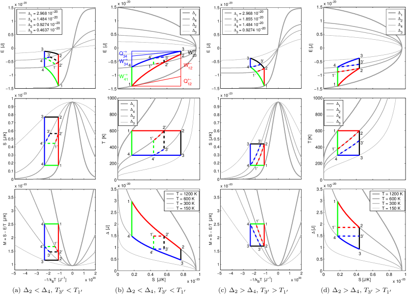
Figure 1: (Color online) Graphs of thermodynamic equilibrium properties of a spin-1/2 system. (a) and (c): graphs of energy $E$, entropy $S$, Massieu function $M=S-(E/T)$ versus $-1/k_{\rm\scriptscriptstyle B}T$ at four values of the energy-level gap $\Delta$. (b) and (d): graphs of energy $E$ and temperature $T$ versus entropy $S$ at four values of $\Delta$, and of energy-level gap $\Delta$ versus $S$ at four values of temperature. The four values of $\Delta$ in (a) and (b) correspond to magnetic field intensities of 1600, 500, 250, and 800 T, respectively; in (b) and (d) of 1600, 1000, 500, and 800 T (these extremely large values are chosen for ease of visualization at ordinary temperatures and intermediate entropies). On each graph, the 1-2-3-4 paths represents a Carnot cycle: isotherm 1-2 at $T_{\rm high}=600$ K, isoentropic 2-3, isotherm 3-4 at $T_{\rm low}=300$ K, isoentropic 4-1. For these cycles, $Q^{\leftarrow}_{12}=T_{\rm high}(S_{2}-S_{1})$, $W^{\leftarrow}_{12}=E_{2}-E_{1}-Q^{\leftarrow}_{12}$, $W^{\leftarrow}_{23}=E_{3}-E_{2}$, $Q^{\rightarrow}_{34}=T_{\rm low}(S_{2}-S_{1})$, $W^{\rightarrow}_{34}=E_{3}-E_{4}-Q^{\rightarrow}_{34}$, $W^{\rightarrow}_{41}=E_{4}-E_{1}$ and, therefore, $W^{\rightarrow}_{\rm net,1234}=W^{\rightarrow}_{34}+W^{\rightarrow}_{41}-W^{\leftarrow}_{12}-W^{\leftarrow}_{23}=(T_{\rm high}-T_{\rm low})(S_{2}-S_{1})=Q^{\leftarrow}_{12}[1-(T_{\rm low}/T_{\rm high})]$. The 1’-2’-3’-4’ paths [2’=2 and 4’=4 in (c) and (d)] represent instead an Otto-type cycle of the kind considered in Refs. Feldmann ; Kieu : iso-energy-gap process 1’-2’ with $T\leq T_{\rm high}=600$ K, isoentropic 2’-3’, iso-energy-gap 3’-4’ with $T\geq T_{\rm low}=300$ K, isoentropic 4’-1’. For these Otto-type cycles, $\Delta_{1^{\prime}}=\Delta_{2^{\prime}}=\Delta^{\prime}_{\rm high}=\max(\Delta_{2},\Delta_{4})$, $\Delta_{3^{\prime}}=\Delta_{4^{\prime}}=\Delta^{\prime}_{\rm low}=\min(\Delta_{2},\Delta_{4})$, $Q^{\leftarrow}_{1^{\prime}2^{\prime}}=E_{2^{\prime}}-E_{1^{\prime}}$, $W^{\rightarrow}_{4^{\prime}1^{\prime}}=E_{4^{\prime}}-E_{1^{\prime}}=E_{1^{\prime}}[(\Delta^{\prime}_{\rm low}/\Delta^{\prime}_{\rm high})-1]$, $W^{\leftarrow}_{2^{\prime}3^{\prime}}=E_{3^{\prime}}-E_{2^{\prime}}=E_{2^{\prime}}[(\Delta^{\prime}_{\rm low}/\Delta^{\prime}_{\rm high})-1]$ and, therefore, $W^{\rightarrow}_{\rm net,1^{\prime}2^{\prime}3^{\prime}4^{\prime}}=W^{\rightarrow}_{4^{\prime}1^{\prime}}-W^{\leftarrow}_{2^{\prime}3^{\prime}}=Q^{\leftarrow}_{1^{\prime}2^{\prime}}[1-(\Delta^{\prime}_{\rm low}/\Delta^{\prime}_{\rm high})]$.

Each graph in Figure 1 shows a Carnot cycle, i.e., a sequence of an isothermal process 1-2 at a high temperature $T_{\rm high}$, an isoentropic 2-3, another isothermal process at a temperature $T_{\rm low}<T_{\rm high}$, and another isoentropic 4-1. Because $S=S(\Delta/T)$ ($S$ decreasing with $\Delta/T$ for $T>0$), it is clear that the isoentropic changes between $T_{\rm low}$ and $T_{\rm high}$ and the isothermal changes between $S_{1}=S_{4}$ and $S_{2}=S_{3}$ are possible only by changing the energy-level gap $\Delta$. Therefore, to have $S_{2}>S_{1}$, we need $\Delta_{2}/T_{\rm high}=\Delta_{3}/T_{\rm low}<\Delta_{4}/T_{\rm low}=\Delta_{1}/T_{\rm high}$, i.e.,

$$\frac{\Delta_{\rm high}}{\Delta_{\rm low}}\left[\frac{T_{\rm low}}{T_{\rm high}}\right]^{2}\!\!=\frac{\Delta_{4}}{\Delta_{2}}>\frac{\Delta_{4}}{\Delta_{1}}=\frac{T_{\rm low}}{T_{\rm high}}=\frac{\Delta_{3}}{\Delta_{2}}>\frac{\Delta_{\rm low}}{\Delta_{\rm high}}\ ,$$ (17)

where, noting that $\Delta_{3}<\Delta_{2}<\Delta_{1}$ and $\Delta_{3}<\Delta_{4}<\Delta_{1}$, we set $\Delta_{\rm low}=\Delta_{3}$ and $\Delta_{\rm high}=\Delta_{1}$. Relations (17) imply (see also Figure legend) general bounds on the net-work to high-temperature-heat ratio (Carnot coefficient),

$$1-\frac{\Delta_{\rm high}}{\Delta_{\rm low}}\left[\frac{T_{\rm low}}{T_{\rm high}}\right]^{2}\!\!<\frac{W^{\rightarrow}_{\rm net,1234}}{Q^{\leftarrow}_{12}}=1-\frac{T_{\rm low}}{T_{\rm high}}<1-\frac{\Delta_{\rm low}}{\Delta_{\rm high}}\ .$$ (18)

Notice that $\Delta_{2}\gtrless\Delta_{4}$ depending on whether $\Delta_{\rm low}/\Delta_{\rm high}\gtrless(T_{\rm low}/T_{\rm high})^{2}$. Indeed, we may choose arbitrarily $T_{\rm high}$, $T_{\rm low}<T_{\rm high}$, $\Delta_{\rm high}=\Delta_{1}$, and $\Delta_{\rm low}=\Delta_{3}<\Delta_{\rm high}T_{\rm low}/T_{\rm high}$. Then, we must set $\Delta_{2}=\Delta_{\rm low}T_{\rm high}/T_{\rm low}$ and $\Delta_{4}=\Delta_{\rm high}T_{\rm low}/T_{\rm high}$. So, if we choose $\Delta_{\rm low}=\Delta_{\rm high}(T_{\rm low}/T_{\rm high})^{2}$, $\Delta_{2}=\Delta_{4}$ and we obtain a Carnot cycle between only three values of $\Delta$.

Of course, if the cycle is reversed, we obtain, instead of a heat-engine effect, a refrigeration or heat-pump effect.

Each graph in Figure 1 shows also an Otto-type cycle Feldmann ; Kieu bound by the same $T_{\rm high}$ and $T_{\rm low}$, i.e., a sequence of an iso-energy-gap process 1’-2’ at $\Delta^{\prime}_{\rm high}$, an isoentropic 2’-3’, another iso-energy-gap process 3’-4’ at $\Delta^{\prime}_{\rm low}$, and another isoentropic 4’-1’. Here, the fact that $S=S(\Delta/T)$ is a decreasing function of $\Delta/T$ for $T>0$, implies that to have $S_{2^{\prime}}>S_{1^{\prime}}$, we need $\Delta^{\prime}_{\rm high}/T_{\rm high}=\Delta^{\prime}_{\rm low}/T_{3^{\prime}}<\Delta^{\prime}_{\rm high}/T_{1^{\prime}}=\Delta^{\prime}_{\rm low}/T_{\rm low}$, i.e.,

$$\frac{T_{\rm high}}{T_{\rm low}}\left[\frac{\Delta^{\prime}_{\rm low}}{\Delta^{\prime}_{\rm high}}\right]^{2}\!\!=\frac{T_{3^{\prime}}}{T_{1^{\prime}}}>\frac{T_{3^{\prime}}}{T_{\rm high}}=\frac{\Delta^{\prime}_{\rm low}}{\Delta^{\prime}_{\rm high}}=\frac{T_{\rm low}}{T_{1^{\prime}}}>\frac{T_{\rm low}}{T_{\rm high}}\ .$$ (19)

Relations (19) imply (see also Figure legend) general bounds on the net-work to high-temperature-heat ratio,

$$1-\frac{T_{\rm high}}{T_{\rm low}}\left[\frac{\Delta^{\prime}_{\rm low}}{\Delta^{\prime}_{\rm high}}\right]^{2}\!\!<\frac{W^{\rightarrow}_{\rm net,1^{\prime}2^{\prime}3^{\prime}4^{\prime}}}{Q^{\leftarrow}_{1^{\prime}2^{\prime}}}=1-\frac{\Delta^{\prime}_{\rm low}}{\Delta^{\prime}_{\rm high}}<1-\frac{T_{\rm low}}{T_{\rm high}}\ .$$ (20)

Notice that $T_{3^{\prime}}\gtrless T_{1^{\prime}}$ depending on whether $(\Delta^{\prime}_{\rm low}/\Delta^{\prime}_{\rm high})^{2}\gtrless T_{\rm low}/T_{\rm high}$, so that if we choose $(\Delta^{\prime}_{\rm low}/\Delta^{\prime}_{\rm high})^{2}=T_{\rm low}/T_{\rm high}$, $\Delta_{2}=\Delta_{4}$ and we obtain a special Otto-like cycle with $T_{3^{\prime}}=T_{1^{\prime}}$ and efficiency $1-(T_{\rm low}/T_{\rm high})^{1/2}$. Notice also that in terms of the iso-energy-level gaps of the Carnot cycle that circumscribes the Otto cycle, the case $T_{3^{\prime}}>T_{1^{\prime}}$ obtains for $(T_{\rm low}/T_{\rm high})^{5/2}<\Delta_{\rm low}/\Delta_{\rm high}<(T_{\rm low}/T_{\rm high})^{3/2}$. In this range, the Otto cycle cannot be run in reverse (refrigeration or heat-pump) mode between two heat baths, for in such mode the hot bath temperature must be at most $T_{1^{\prime}}$ and the cold bath at least $T_{3^{\prime}}$.

Because the iso-energy-gap processes (iso-magnetic field for spin-1/2 system) which characterize the Otto-type cycle are not isotherms, if they are obtained Kieu by contacts with heat baths at $T_{\rm high}$ and $T_{\rm low}$, respectively, they involve entropy generation due to irreversibility resulting from the heat exchange [see Eq. (16)] across a large temperature difference (decreasing as $T_{1^{\prime}}\rightarrow T_{\rm high}$ and $T_{3^{\prime}}\rightarrow T_{\rm low}$). These and other realistic irreversibilities are modeled in Ref. Feldmann with a Kossakowski-Lindblad-type linear dissipative term in the quantum dynamical law, as a means to describe relaxation to equilibrium and decoherence, required for example to decouple the system from the heat source, i.e., to model dynamically the heat interactions. The only way to avoid these inefficiencies is the impractical (infinite) sequence of infinitesimal contacts with heat baths at different temperatures in the ranges $T_{1^{\prime}}\div T_{\rm high}$ and $T_{3^{\prime}}\div T_{\rm low}$.

In this paper, instead, by showing the feasibility of a Carnot cycle for a two-level system, with no need of sequences of infinitesimal heat exchanges with an infinite number of heat baths, we show that the quantum nature of the working substance does not impose any fundamental bound, other than the celebrated Carnot bound, to the thermodynamic efficiency of heat-to-work conversion when two different temperature thermal reservoirs are available. The possibility of engineering simultaneously heat and work interactions as needed for the isotherms of the Carnot cycle seems within reach of current experiments, e.g., via a maser-laser tandem technique Scully . The Carnot cycle “efficiency” is higher, as it should, than that of the ’inscribed’ Otto-like cycle at the center of recent studies Scully ; Lloyd ; He ; Kieu ; Kosloff ; Feldmann .

Only twenty years ago quantum thermodynamics and pioneering proposals to incorporate the second law of thermodynamics into the quantum level of description were considered “adventurous” schemes Nature . Discussions in quantum terms of old thermodynamic problems such as that of “unitary accessibility” Allahveryan or of defining entropy for non-equilibrium states, were perceived as almost irrelevant speculations. Today’s experimental techniques bring thermodynamics questions back to the forefront of quantum theory. Remarkably, the rigorous application of energy and entropy balances, provides ideas and guidance, and the second law remains a perpetual source of inspiration towards the discovery of new physics.

References

• (1) M.O. Scully, Phys. Rev. Lett. 88, 050602 (2002).
• (2) S. Lloyd, Phys. Rev. A 56, 3374 (1997); S. Lloyd and W.H. Zurek, J. Stat. Phys. 62, 819 (1991).
• (3) J. He, J. Chen, and B. Hua, Phys. Rev. E 65, 036145 (2002); C.M. Bender, D.C. Brody, and B.K. Meister, J. Phys. A 33, 4427 (2000).
• (4) T.D. Kieu, Phys. Rev. Lett. 93, 140403 (2004).
• (5) E. Geva and R. Kosloff, J. Chem. Phys. 96, 3054 (1992), 97, 4398 (1992), 104, 7681 (1996); R. Kosloff, E. Geva, and J. Gordon, J. Appl. Phys. 87, 8093 (2000).
• (6) T. Feldmann and R. Kosloff, Phys. Rev. E 70, 046110 (2004), and references therein.
• (7) H. Scovil and E.O. Schulz-Dubois, Phys. Rev. Lett. 2, 262 (1959); J.E. Geusic, E.O. Schulz-Dubois, and H. Scovil, Phys. Rev. 156, 343 (1967), and references therein.
• (8) E.M. Purcell and R.V. Pound, Phys. Rev. 81, 279 (1951).
• (9) N.F. Ramsey, Phys. Rev. 103, 20 (1956).
• (10) J.P. Gordon, H.J. Zeiger, and C.H. Townes, Phys. Rev. 95, 282 (1954).
• (11) W.H. Zurek, Rev. Mod. Phys. 75, 715 (2003).
• (12) S. Gheorghiu-Svirschevski, Phys. Rev. A 63, 54102 (2001), and references therein.
• (13) A.E. Allahverdyan, R. Balian, and T.M. Nieuwenhuizen, Europhys. Lett. 67, 565 (2004); but the problem of unitary accessibility is first addressed in G.N. Hatsopoulos and E.P. Gyftopoulos, Found. Phys. 6, 127 (1976) and defines what engineers call “adiabatic availability”.
• (14) J. Maddox, Nature 316, 11 (1985).
• (15) G.P. Beretta, Phys. Rev. E 73, 026113 (2006).