Quantum Circuit Placement

Abstract

We study the problem of the practical realization of an abstract quantum circuit when executed on quantum hardware. By practical, we mean adapting the circuit to particulars of the physical environment which restricts/complicates the establishment of certain direct interactions between qubits. This is a quantum version of the classical circuit placement problem. We study the theoretical aspects of the problem and also present empirical results that match the best known solutions that have been developed by experimentalists. Finally, we discuss the efficiency of the approach and scalability of its implementation with regards to the future development of quantum hardware.

1 Introduction

Quantum algorithm design is usually done in an abstract model of computation with the primary interest being the development of efficient algorithms (e.g. polynomial versus exponential sized circuits) independently of the details of the potential physical realization of the related quantum circuits. Theoretical quantum computational architectures usually, for convenience, assume that it is possible to directly interact any two physical qubits. It is well known that in physical implementations direct interactions between two distinct qubits may sometimes be hard if not impossible to establish. For instance, it is not uncommon for an interaction to have less than $0.2$ Hz frequency (e.g. carbons C2 and C6 from [20]), while the decoherence may take around one second. This means that the interaction between such qubits will be essentially seen as noise. A physical realization of a quantum processor can of course indirectly couple any two qubits, with some overhead cost. However, in practice this can be very costly (and, for example, make the implementation infeasible with available technology), and so one needs to find a way to minimize this overhead, which we will refer to as quantum circuit placement problem.

Some authors [18] try to avoid long interactions by considering the linear nearest neighbor computational architecture where all qubits are lined up in a chain (such as trapped ions [9]) and only the nearest neighbors are allowed to interact. Mathematically, for a system with $n$ qubits $q_{1},\;q_{2},...\;,q_{n}$, the 2-qubit gates are allowed on qubits whose subscript values differ by one. Such an architecture, however, does not necessarily represent reality. For instance, in NMR technologies the fastest interactions will not usually form a chain. In a 3-qubit computation, the fastest interactions can be aligned to form a chain (acetyl chloride, Figure 1, [14]) or a complete graph [6]. In all molecules used in NMR and known to the authors that employ four or more qubits, the fastest interactions are established along the chemical bonds and they do not form a single chain. The chain nearest neighbor architecture can apply to some quantum dot based architectures and certain variations of trapped ion [9] quantum technologies, but does not represent the reality behind other technologies, including those based on NMR, Josephson junctions, optical technology, and certain other variations of trapped ions [19]. Furthermore, we are unaware of any automated procedure for optimizing the interactions even if the latter are restricted to the chain nearest neighbor architecture.

It has been recently proposed to use EPR pairs to teleport logic qubits in a Kane model [23] when long-distance swapping of a single value becomes too expensive [3]. However, this type of “technology mating” may not always be possible. For instance, it seems hard if not impossible to mate NMR with an optic EPR source while doing a computation on an NMR machine. It is also not obvious how congested such an architecture gets if simultaneous teleporting of a large number of qubits is required. We concentrate on an approach that does not require mating different technologies, and is technology independent.

At roughly the same time as our initial publication there was another publication devoted to the study of quantum circuit placement problem [25]. Both papers, [25] and ours consider the problem of placement in the quantum circuit computational model. The major difference that sets the two research directions apart and yet shows that the results are complementary is in our paper we consider pre-given architectures, whereas [25] forms an architecture on the fly according to the circuit that needs to be implemented.

Unlike in the quantum case, the classical circuit placement problem is very well known and extensively studied [15]. Classical circuit placement is concerned primarily with minimizing the total wirelength, power, and congestion. Timing minimization is considered to be a secondary optimization objective. In quantum technologies, placement is equivalent to timing optimization under the natural assumption that gate fidelities [21] are inversely proportional to the coupling strength/gate runtime, otherwise, a function of both may be considered. However, timing minimization for quantum versus CMOS technologies are two distinct and dissimilar problems. This is not surprising given the conceptual differences in the two computational models. A quantum circuit placer cannot be constructed by reusing the existing EDA tools and thus, must be built from scratch.

In practice and at present, the mapping of qubits in a circuit into physical qubits is done by hand, but as the quantum computations scale, a more robust (automated) technique for such a mapping must be employed. In this paper, we study the problem of mapping a circuit into a physical experiment where we wish to optimize the interactions. We formulate this problem mathematically and study its complexity. Given the problem of finding an optimal assignment of qubits is unlikely to have a polynomial time optimal solution, as it is NP-Complete, and exhaustive search requires $n!$ tries for an $n$-qubit system, we develop a heuristic-based algorithm. We verify the latter on data taken from existing quantum experiments.

Throughout the text, and especially in the experimental results section, we refer to liquid state NMR technology for quantum computation. While there are certain problems with using liquid state NMR to work with over 10 qubits [5, 11, 20], so far, it is the best developed methodology for quantum computing experiments. Liquid state NMR experiments provide a nice data set for both the interaction frequencies and the circuits of interest, and a test bed for development of suitable scalable spin-based quantum computing devices. While we use results from the liquid state NMR experiments, it is important to emphasize that our approach is not restricted to a particular technology. For instance, many circuits we consider are composed for the Ising type Hamiltonian, however, Ising type Hamiltonian describes not only the liquid state NMR experiments, but also certain superconductivity proposals [8].

The remainder of the paper is organized as follows. We start with a basic overview of quantum computation and description of quantum circuits, in Section 2. Following this, in Section 3, we formally define the objects we will be working with and formulate the circuit placement problem. We next study the complexity aspect of the circuit placement problem, and conclude that even a simplified version of this problem is NP-Complete, refer to Section 4. Thus, for the purpose of having an efficient practical solution to the placement problem we need to concentrate on heuristic solutions. Our heuristics, described in Section 5, consist of two algorithms: determining an efficient placement of individual subcircuits, and permuting the qubit values to interconnect placed subcircuits. We conclude this section with the description of our quantum circuit placement software package. In Section 6 we describe a number of experiments that test quality, efficiency, and scalability of our heuristic solution. Concluding remarks can be found in Section 7.

2 Preliminaries

We present a short review of the basic concepts of quantum computation. For a more detailed introduction, please see [21].

The key ingredients of the standard quantum computation model are the data structure (described by state vectors), the set of possible transformations allowing one to perform a desired calculation (unitary matrices), and the access to the result of a computation (measurement). In very basic terms, every quantum algorithm begins with a state initialization, followed by a computational stage, and ends with a measurement. The description of the state vectors, unitary matrices, and quantum measurement is the focus of the following discussion.

The state of a single qubit is a linear combination $\alpha_{0}|0\rangle+\alpha_{1}|1\rangle$ (which can also be written as $\sum_{x\in\{0,1\}}\alpha_{x}|x\rangle$) in the basis $\{|0\rangle,\;|1\rangle\}$, called the state vector, where $\alpha_{0}$ and $\alpha_{1}$ are complex numbers such that $|\alpha_{0}|^{2}+|\alpha_{1}|^{2}=1$. The real numbers $|\alpha_{0}|^{2}$ and $|\alpha_{1}|^{2}$ represent the probabilities of reading the “pure” logic states $|0\rangle$ and $|1\rangle$ upon measurement. The state of a quantum system with $n>1$ qubits is given by an element of the tensor product of the single state spaces and can be represented by a normalized vector of length $2^{n}$ (state vector), as $\sum_{x\in\{0,1\}^{n}}\alpha_{x}|x\rangle$, where $\sum_{x\in\{0,1\}^{n}}|\alpha_{x}|^{2}=1$. Each of the real numbers $|\alpha_{x}|^{2}$ represents the probability of finding the quantum mechanical system in the state $|x\rangle$. As such, measurement gives probabilistic access to $n$ bits of classical information. According to the laws of quantum mechanics, a quantum system evolution allows changes of the state vector through its multiplication by $2^{n}\times 2^{n}$ unitary matrices (a square matrix $U$ over complex numbers is called unitary iff $UU^{\dagger}=I$, where $U^{\dagger}$ is the complex conjugate of $U$).

For example, a 2-qubit quantum mechanical system described by the state vector $\vec{v}=|10\rangle$ (the result of the measurement of this state is deterministic, since there is only one non-zero coordinate) may be acted on by a unitary matrix of appropriate dimension (in this case, $2^{n}|_{n=2}=2^{2}=4$)

$$U=\frac{1}{2}\left(\begin{array}[]{rrrr}1&1&1&1\\ 1&i&-1&-i\\ 1&-1&1&-1\\ 1&-i&-1&i\end{array}\right).$$ (1)

This results in the transformation $\vec{v}\mapsto U\vec{v}$ computed as follows:

$\vec{v}=|10\rangle=0*|00\rangle+0*|01\rangle+1*|10\rangle+0*|11\rangle=\left(\begin{array}[]{r}0\\ 0\\ 1\\ 0\end{array}\right)\mapsto$ $U\vec{v}=\frac{1}{2}\left(\begin{array}[]{rrrr}1&1&1&1\\ 1&i&-1&-i\\ 1&-1&1&-1\\ 1&-i&-1&i\end{array}\right)\left(\begin{array}[]{r}0\\ 0\\ 1\\ 0\end{array}\right)$
$=\frac{1}{2}\left(\begin{array}[]{r}1\\ -1\\ 1\\ -1\end{array}\right)=\frac{1}{2}(|00\rangle-|01\rangle+|10\rangle-|11\rangle).$

With this state, the result of measurement gives $|00\rangle$, $|01\rangle$, $|10\rangle$ and $|11\rangle$ with equal probabilities. In fact, with this example we have illustrated application of the 2-qubit Quantum Fourier Transform to the basis state $|10\rangle$.

The above shows how a state vector evolves under the action of a unitary transformation. In practice, a desired unitary transformation will need to be decomposed into primitive operations that can be implemented in hardware. At the experimental level, these primitive operations, or elementary gates, are usually defined in terms of the Hamiltonian (which describes the energy of a quantum mechanical system), and depends on a particular implementation/technology. While our placement algorithms/theory and program implementation readily support any gate library, we next introduce some of the particular gates used in the examples included in this paper (in fact, the following family of gates forms a complete library).

• single qubit rotation gates $R_{x}(\theta):=\left(\cos(\frac{\theta}{2})\;\;\;\;\;-i\sin(\frac{\theta}{2})\atop-i\sin(\frac{\theta}{2})\;\;\;\;\,\cos(\frac{\theta}{2})\right)$, $R_{y}(\theta):=\left(\cos(\frac{\theta}{2})\;\;\;\;-\sin(\frac{\theta}{2})\atop\sin(\frac{\theta}{2})\;\;\;\;\;\;\;\cos(\frac{\theta}{2})\right)$, and $R_{z}(\theta):=\left(e^{-i\theta/2}\;\;\;\;\;\;0\atop 0\;\;\;\;\;\;\;\;\;e^{i\theta/2}\right)$;

• two-qubit interaction gate
  $ZZ(\theta):=\left(\begin{array}[]{rrrr}e^{-i\theta/2}&0&0&0\\ 0&e^{i\theta/2}&0&0\\ 0&0&e^{i\theta/2}&0\\ 0&0&0&e^{-i\theta/2}\end{array}\right)$.

In liquid state NMR, single qubit $R_{x}$ and $R_{y}$ gates are implemented by radio frequency (RF) pulses in the $X$-$Y$ plane (in the lab setting this usually corresponds to the horizontal plane of the physical 3D space we live in). The $R_{z}$ gates are implemented by a change of the so-called rotating reference frame and require no action/waiting. From the designer’s perspective this means that the $R_{z}$ gates are “free”. Finally, $ZZ$ gates are a part of the drift Hamiltonian, meaning they happen as a natural evolution of the system and must be waited for until completion. Those $ZZ$ interactions/gates that are not needed in a computation get eliminated via a technique called refocussing.

In particular, in terms of the NMR gates, the matrix in equation (1) can be decomposed into the matrix product

$$I\otimes R_{x}(\pi)\;\cdot\;I\otimes R_{z}(\pi)\;\cdot\;I\otimes R_{y}(-\frac{\pi}{2})\;\cdot\;R_{z}(-\frac{3\pi}{4})\otimes R_{z}(-\frac{3\pi}{4})$$

$$\cdot\;ZZ(-\frac{\pi}{4})\;\cdot\;R_{y}(\frac{\pi}{2})\otimes I\;\cdot\;R_{z}(-\pi)\otimes I\;\cdot\;R_{x}(\pi)\otimes I$$

up to the global phase (i.e., constant factor) $e^{i\pi/8}$ and a permutation of the output qubits, both of which are insignificant considerations from the point of view of the computation that needed to be performed. Note, that the circuit associated with the above implementation requires only four pulses and uses only one two-qubit gate. This circuit representation was specifically optimized for the liquid state NMR implementation.

Liquid state NMR works in a weak interaction mode, meaning the two-qubit $ZZ$ gate takes much longer (e.g., often on the order of 10 times longer) to be applied than a single qubit gate. Thus, careful assignment of the interactions used in the computation is crucial in terms of the efficient execution of a logical quantum circuit on a physical quantum mechanical system; this is the topic of study addressed in the present paper.

Finally, note that $ZZ(\pi/2)$ is equivalent to CNOT (a commonly used gate that transforms basis states according to the formula $|a\;\;b\rangle\mapsto|a\;\;a\oplus b\rangle$, and extends to other quantum states by linearity) up to single qubit rotations. This means that every circuit with single qubit and CNOT gates can be easily rewritten in terms of single qubit rotations $R_{x}$, $R_{y}$ and $R_{z}$, and the $ZZ(\pi/2)$ gates, and such a rewriting operation does not change a particular instance of the associated placement problem.

3 Formalization of the circuit mapping problem

Circuits devised by researchers in the area of quantum computing are very often written in terms of a single qubit and two-qubit gates. Thus, any circuit with gates spanning over more than two qubits is first translated into a circuit with a single qubit and two qubit gates. We assume such a circuit as input. Next, most of the practical circuits are levelled, that is the gates that can be applied in parallel appear at one logic level (in circuit diagrams: directly below or above other gates from the same level). Levelization helps to reduce the overall runtime of the circuit, and thus it is a desired operation at the time the circuit is synthesized.

Before the circuit’s qubits (i.e. logical qubits) are mapped into the molecule’s nuclei (i.e. physical qubits) and the exact delays are known, it is hard to decide how long it will take to execute a single gate and take it into account while trying to minimize the delay of the entire circuit. This means that the circuit’s qubits must be mapped to the molecule’s nuclei first.

In a practical setting and according to how it is done in current experiments the first step is to efficiently assign qubits to nuclei. In the existing NMR tools, the timing optimization is built into a compiler [2] that takes in a circuit and a refocusing scheme and outputs a sequence of (timed) pulses ready to be executed. This is the last step before the circuit gets executed and before it is done the logical qubits must be assigned to the nuclei.

In practice, it is a natural assumption that gates from the next level can start being executed before execution of the current level has completed. The total runtime is defined as the time spent by a circuit between the input initialization and measurement of the output. With the assumptions made, the runtime of a circuit composed of gates $G[1],G[2],...,G[k]$ can be found by the following dynamic programming algorithm.

Create array Time[1..n], initiate its elements to 0;
for i=1..k
  if G[i] is a 2-qubit gate built on qubits t and c
    time[c]:=
       max{time[c],time[t]}+GateOperatingTime(G[i]);
    time[t]:=time[c];
  else // else gate G[i] is a single qubit gate that operates on qubit t
    time[t]:=time[t]+GateOperatingTime(G[i]);
  end if;
end for;
return max{time[1..n]}; // maximally busy qubit is the one that finishes the job last

Circuit runtime calculation in a computational model where logic levels need to be executed sequentially is also supported by the theory we develop and our program implementation. We next introduce the following notations/definitions.

Definition 1.

A physical environment (molecule) is a complete non-oriented graph with a finite set of vertices (nuclei) $\{v_{1},v_{2},$ $...\;,v_{m}\}$ and weighted edges $\{(v_{i},v_{j})\}_{1\leq i\leq j\leq m}$ with $W(v_{i},v_{j})\geq 0$.

Weights $W(v_{i},v_{j})$ are proportional to the inverse of the coupling frequency (for two qubit gates) and the inverse of nuclei processing frequencies (for single qubit gates). In other words, they indicate how long it takes to apply a fixed angle 2-qubit gate (in case of edge $(v_{i},v_{j})$, $i\neq j$) or a fixed angle single qubit gate (in case of edge $(v_{i},v_{i})$).

Definition 2.

A quantum circuit is built on $n$ qubits $q_{1},q_{2},...$ $,q_{n}$ and consists of a finite number of levels $L_{1},L_{2},...\;,L_{k}$, where each level $L_{i}$ is a set of one or two qubit gates $G_{i}^{1},G_{i}^{2},...,G_{i}^{t_{i}}$. Each gate has a weight function $T(G_{i}^{j})$ that indicates how long it takes this gate to use the interaction defined by the qubits it operates on .

Definition 3.

The quantum circuit placement problem is to construct an injective (one-to-one) function $P:\{q_{1},$ $q_{2},...\;,q_{n}\}\mapsto\{v_{1},v_{2},...\;,v_{m}\}$ such that with this mapping the runtime of a given circuit is minimized. The gate’s $G(q_{i},q_{j})$ execution cost is defined by the mapping $q_{i}\mapsto v_{i}$, $q_{j}\mapsto v_{j}$ according to the formula

$$GateOperatingTime(G(q_{i},q_{j})):=W(v_{i},v_{j})*T(G(q_{i},q_{j})).$$

There are $\frac{\displaystyle m!}{\displaystyle(m-n)!}$ potential candidates for an optimal matching. Thus, a simple minded exhaustive search procedure will require runtime at least $O(\frac{\displaystyle m!}{\displaystyle(m-n)!})$, counting a singe operation per each possible assignment.

Example 1.

Illustrated in Figure 1(a) is the acetyl chloride molecule and a table with the chemical shifts/coupling strengths (in liquid state NMR) [14]. The chemical shifts and coupling strengths were recalculated into the delays needed to apply 90-degree rotations in the $X$-$Y$ plane (single qubit rotations around the axis $Z$ are “free” in that they are done by changing the rotating reference frame [13] and require no pulse or a delay associated with respect to their application [5]) and a 90-degree $zz$-rotation (2 qubit gate). The delays are measured in terms of $\frac{1}{10000}\;sec$, and are rounded to keep the numbers integer. Figure 1(b) describes liquid state NMR computational properties of the molecule in graph form.

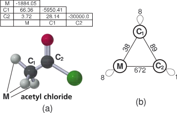
Figure 1: (a) acetyl chloride molecule with three spin-$\frac{1}{2}$ nuclei used as qubits: $M$ (three hydrogens that share the same chemical environment and thus appear practically indistinguishable), $C_{1}$ and $C_{2}$ (both are carbons) and (b) graph representation of interactions between qubit nuclei of this molecule.

Example 2.

Illustrated in Figure 2 is a circuit (in terms of NMR pulses) for the encoding part of the 3-qubit quantum error correction code taken from [14]. It consists of a number of single qubit and two qubit gates. Gates $R_{y}(90)$ require an RF pulse of the length proportional to the degree of rotation. Since the degree of rotation is $90$, $T(R_{y}(90))=1$. In liquid state NMR gates $R_{z}(90)$ and $R_{z}(-90)$ can be applied through the change of rotating reference frame and require no delay. Thus, $T(R_{z}(90))=T(R_{z}(-90))=0$. Both $zz$-interactions are $90$-degree, therefore $T(ZZ(90))=1$.

Figure 2: Encoding part of the 3-qubit error correcting code.

Example 3.

Let us consider the placement problem of the 3-qubit encoding quantum circuit (Figure 2) into acetyl chloride (Figure 1). There are $3!=6$ possible placement assignments. One possible placement is the following: $a\rightarrow M,\;b\rightarrow C_{2}$ and $c\rightarrow C_{1}$. The circuit runtime calculation is illustrated in Table 1 for steps $i=1..5$ appearing in columns 2-6 and the first column listing the available qubits. Single qubit rotations around $Z$ axis are ignored since their contribution to the runtime is zero. The circuit runtime equals the largest number in the last column, 770. This example placement is not optimal. The minimal possible value of runtime is equal to $136$, and is achieved by the placement $a\rightarrow C_{2},\;b\rightarrow C_{1},\;c\rightarrow M$.

Table 1: Cost of $\{a\rightarrow M,\;b\rightarrow C_{2},\;c\rightarrow C_{1}\}$ mapping.

$time[\;]$	$Y_{a}$90	$ZZ_{ab}$90	$Y_{c}$90	$ZZ_{bc}$90	$Y_{b}$90
a	8	680	680	680	680
b	0	680	680	769	770
c	0	0	8	769	769

4 Complexity

In this section we show that the placement problem is NP-Complete, and thus for practical purposes we need to focus on heuristic solutions. In particular, we consider the problem of finding a Hamiltonian cycle in a graph $H=(V_{H},E_{H})$. We next formulate a mapping problem whose solution is equivalent to the solution of a Hamiltonian cycle problem.

Let the physical environment be a graph with the same set of vertices as graph $H$, $\{v_{1},v_{2},...\;,v_{m}\}$. Edge $(v_{i},v_{j})$ of the physical environment has weight one if and only if $(v_{i},v_{j})$ is not an edge of graph $H$. All other edges have weight zero. The physical environment, as defined, models the graph $H$ from the Hamiltonian cycle problem. Let the quantum circuit consist of $m$ levels and be built on $m$ qubits $\{q_{1},q_{1},...\;,q_{m}\}$. Let the $i^{\textrm{th}}$ level be composed of a single 2-qubit gate $G(q_{i},q_{(i\bmod m)+1})$ with $T(G)=1$. The runtime of the circuit is thus the sum of the execution runtimes of its gates. The defined quantum circuit models the Hamiltonian cycle. When the quantum circuit is mapped into the physical environment such that its runtime is minimized, the minimal possible value of runtime, which is zero, is possible to achieve if and only if the physical environment has a Hamiltonian cycle that goes along the edges with zero weight. This is equivalent to $H$ having a Hamiltonian cycle.

5 Heuristic solution

Before we begin the description of our algorithm, we first make several observations about the quantum information processing proposals and quantum circuits. Firstly, in real world experiments, such as [12, 20], the qubit-to-qubit interactions are usually aligned along the chemical bonds, or otherwise using only the fastest interactions allowed by the physical environment. Secondly, most often a single qubit gate can be executed much faster than a two-qubit gate. Third, it may turn out that a circuit is composed of a number of computations/stages each of which has its own best mapping into a physical environment. If the circuit is treated as a whole, no placement will be efficient because at least one part of such a placement will be inefficient. Below, we describe an approximate placement algorithm that uses heuristics derived from these observations.

5.1 Algorithm

Outline. The idea of our algorithm is to break a given circuit into a number of subcircuits such that an efficient placement can be found for each of the subcircuits. We next connect the individually placed subcircuits to form the desired computation via swapping/permutation circuits.

Preprocessing. We first take the physical environment and establish which interactions are considered the fastest. One method for doing this is to choose a $Threshold$ such that if a value of a qubit-to-qubit interaction is below the $Threshold$, the interaction is considered to be fast, otherwise it is considered too slow and will not be used. The value of the $Threshold$ may be chosen to be the minimal value such that the graph associated with fastest interactions is connected, or may be taken directly from the experimentalists. Either way, we treat the value of the $Threshold$ as a known parameter for our algorithm. Using the $Threshold$ value ensures that our algorithm comes up with a circuit implementation that uses only the fastest interactions.

Algorithm. The algorithm consists of two stages: basic placement and fine tuning, repeated iteratively. In the basic mapping stage we make sure that in some part of the circuit all two qubit gates can be aligned along the fastest interactions of the physical environment. In the fine tuning stage we consider a given subcircuit for which a mapping of circuit qubits into the molecule’s nuclei along the fastest interactions exists. We fine tune this matching by shuffling the solution and taking the actual numbers that represent the length of each gate (including single qubit gates) into account.

We start by reading in the 2-qubit gates from the circuit into a workspace $C$ and do it as long as these gates can be arranged along the fastest interactions provided by the physical environment. As soon as we reach a gate whose addition will prohibit the alignment along the fastest interactions, we stop and concentrate on those gates already in $C$. At this point, we know that the two qubit gates we have read, $g_{1},g_{2},...\;,g_{s}$, can be aligned along the fastest interactions. Take one of such alignments in the case when multiple alignments are possible. The alignment itself can be found by any of the known graph monomorphism techniques, such as [4]. If all monomorphisms can be found reasonably fast (which is true for all experimentally constructed circuits and environments we tried due to their small size/suitable structure), we calculate the circuit runtime for each of them and take the best found. Otherwise, we apply a simple hill climbing algorithm, where for every qubit $q_{i}$ from the circuit such that there exists a two qubit gate $g_{j}$ among those in $C$ that operates on this qubit, try to map it to any of $\{v_{1},v_{2},...\;,v_{m}\}$ and see if this new placement assignment is better than the one provided by the initial matching. If it is, change the way qubit $q_{i}$ is placed, otherwise, move on to the next qubit. Such an operation can be repeated until no improvement can be found or for a set number of iterations. We refer to this step as fine tuning. After the matching is fine tuned, we return to the circuit, erase all the gates from it up to the two qubit gate $g_{s+1}$ that prevented alignment along the fastest interactions at the previous step and repeat the above procedure.

The result of the above algorithm is a finite set of finely tuned placement assignments $P_{1},P_{2},...\;,P_{t}$, but they apply to different subcircuits $C_{1},C_{2},...\;,C_{t}$ of the target circuit. The overall computation looks as follows $C_{1}E_{1,2}C_{2}E_{2,3}...$ $E_{t-1,t}C_{t}$, where $E_{i,i+1}$ is a circuit composed with SWAP gates such that $E_{i,i+1}$ transforms the mapping given by $P_{i}$ into the mapping given by $P_{i+1}$, and initially all qubits are placed according to $P_{1}$.

5.2 Fast permutation circuits

The algorithm from the previous subsection describes all details of the circuit placement, except how to construct circuits $E_{i,i+1}$ that would swap the placement assignment of subcircuit $C_{i}$ into that for $C_{i+1}$. In this subsection we discuss how to compose such circuits efficiently (linear in the number of qubits in the physical environment; and using only the fastest interactions) and solely in terms of SWAP gates.

Problem. For a given permutation (defined as the permutation transforming the placement assignment of subcircuit $C_{i}$ into that for $C_{i+1}$) and a graph defining which two qubits can be interchanged through a single SWAP (such an adjacency graph has an edge between two qubits if it is possible to SWAP their values directly, meaning that the interaction between the two qubits is considered fast), compose a set of SWAPs that realize this permutation.

Observations. Note that the interaction graph is connected.

Assumptions. For simplicity, we assume that all SWAP gates applied to the qubits joined by the edges of adjacency graph $G$ require the same time. Modification of the algorithm presented below that accounts for the actual costs of SWAPs is possible, but it is not discussed here. Next, assume that the graph $G$, as well as its subgraphs, are well separable. That is, there exists a constant $s\in(0,1]$ such that $G$ can be recursively divided into two connected components $G_{1}$ and $G_{2}$, and the ratio of the number of vertices in the smaller subgraph to the number of vertices in the larger subgraph is never less than $s$. In the Appendix we prove that every bounded degree graph with the maximal vertex degree equal $k$ is well separable with parameter $s=\frac{1}{k}$. If we now turn our attention to the possible quantum architectures, we find that it is not physical to believe that there exists a scalable quantum architecture that would allow an unbounded number of direct neighbors. Thus, restricting our attention to bounded degree (and as such, well separable) graphs does not seem to impose any serious restriction. The well separability property certainly holds true for the scalable interaction architectures proposed in the literature: linear nearest neighbor architecture (1D lattice, $s=1/2$), and 2D lattices ($s\geq 1/2$). In our experiments, we found that the interaction graphs for liquid state NMR molecules have $s=1/2$ (which is somewhat better than $s=1/3$ and $s=1/4$ that follow from the theorem in Appendix).

If a number of pairs with different values is to be swapped, the runtime of the experimental implementation of such an operation is associated with the cost of a single SWAP. We make this assumption because in quantum technologies it is possible (not prohibited, and often explicitly possible, such as in liquid state NMR) to execute non-intersecting gates in parallel. Moreover, implementing non-intersecting gates in parallel is not a luxury, rather a necessity for fault-tolerance to be possible [1].

Goal. Our target is to minimize the number of logic levels one needs in order to realize a given permutation as a circuit. Each logic level is composed with a set of non-intersecting SWAPs operating along the fastest interactions defined by the adjacency graph.

Outline. We construct the swapping circuit with the help of a recursive algorithm. At each step our recursion makes sure that certain quantum information has been propagated to its desired location.

Algorithm. Consider adjacency graph $G$ with $n$ vertices that shows which SWAPs can be done directly. Cut this graph into two connected subgraphs $G_{1}$ and $G_{2}$ with the number of vertices equal to or as close to $n/2$ as possible. To do such a cutting we would have to cut a few edges, each called a communication channel.

Consider subgraphs $G_{1}$ and $G_{2}$. Color each vertex white if ultimately (according to the permutation that needs to be realized) we want to see it in $G_{1}$ and black if we want to see it in $G_{2}$. The task is to permute the colors by swapping colors in the adjacent vertices such that all white colored vertices go to the $G_{1}$ part and all black ones move to $G_{2}$. The bottleneck is in how many edges join the two halves $G_{1}$ and $G_{2}$—the number of such edges represents the carrying capacity of the communication channel. This is because all white elements from $G_{2}$ and all black elements from $G_{1}$ must, at some point, use one of such communication channels to move to their subgraph.

If all colored vertices can be brought to their subgraph with a linear cost, $a*n$, then we iterate the algorithm and have the following figure for the complexity of the entire algorithm: $C(n)\leq a*n+C(\frac{n}{s+1}),$ where $C(n)$ is the complexity of the algorithm for a size $n$ problem. The solution for such a recurrence is $C(n)=\frac{a(s+1)n}{s}$. If the graph has separability factor $s=1/2$, the recurrence can be rewritten as $C(n)\leq a*n+C(2n/3)$. The latter has solution

$$C(n)=3a*n+const,$$ (2)

providing a linear upper bound for the entire algorithm.

We next discuss how to move all white vertices into the $G_{1}$ subgraph and, simultaneously, black ones into the $G_{2}$ subgraph in linear time $a*n$. Consider a single subgraph, let us say $G_{1}$, and the edge(s) of $G$ that we cut to create $G_{1}$ and $G_{2}$. First, let us bring all black vertices as close to the communication channel as possible. To do so, we suppose that the communication channel consists of a single edge, otherwise, choose a single edge. We next cut all loops in $G_{1}$ such that in the following solution we will not allow swapping values across all possible edges. After this is done, we have a rooted tree with the root being the unique vertex that belongs to $G_{1}$ and is the end of the communication channel. A rooted tree has a natural partial order to its vertices, induced by the minimal length path from a given vertex to the root.

We next apply the following algorithm. Suppose $G_{1}$ has $k+1$ vertices. At step $i=1..k$, we look at vertices at depth $k-i$ and their parent at depth $k-i-1$. If the vertex at depth $k-i$ is black and its parent is white, we call such a parent a bubble and interchange it with the child through applying a SWAP. We also look at all bubbles introduced on the previous steps. If a bubble has a black child, we SWAP the two (propagate the bubble). Otherwise, all children of the bubble are white, and as a result, this vertex is no longer a bubble. Let us note that once a bubble started “moving”, it will move each step of the algorithm until it is no longer a bubble, which happens only when all its children are white. By the step $i=k$ all potential bubbles have started moving or have already finished their trip. It may take an additional $k$ steps for moving bubbles to finish their movement. By the time step $i=2k$ is completed, every path from a vertex in $G_{1}$ to the root will change color at most once (if color changes it can only change from white to black).

This brings us to the next part: interchanging white and black nodes in $G_{1}$ and $G_{2}$ and actually using the communication channel. We use the communication channel every odd step in this part of the algorithm to bring a single black vertex from $G_{1}$ over to $G_{2}$ and a single white vertex from $G_{2}$ to $G_{1}$. Once a white vertex arrives in $G_{1}$ we call it a bubble and raise it until all its children are white. A similar operation is performed with graph $G_{2}$. Every even step the root vertex of $G_{1}$ is white (and thus is a bubble) and one of its children is black (if all children are white, the algorithm is finished; $G_{1}$ is guaranteed to contain only white vertices, and all of them). We propagate the bubble to one of its children to have a black vertex ready for the next transfer. To get all white nodes to their side we will need at most $2k$ swaps ($k$ because there cannot be more than $k$ white nodes missing, and $*2$ because we use communication channel every second time).

Thus, the total cost of bringing white nodes to $G_{1}$ and black ones to $G_{2}$ is $2k+2k=4k$. Since in the graphs we consider $s\geq 1/2$, the above expression gives an upper bound of $a=8/3$. Substituting this into the recurrence solution (2) gives the upper bound of $8n+const$ for the number of levels in a quantum circuit composed with SWAPs working with the fastest interactions and realizing a given permutation. By considering the permutation $(n,2,3,...,n-1,1)$ and the chain nearest neighbor architecture we can show that the above algorithm is asymptotically optimal.

Physical interpretation. The above formulated algorithm can be interpreted in terms of elementary physics. One can think of a graph as a container with a rather unusual shape (whatever the shape of the graph is when it is drawn), black nodes contain liquid, white nodes—air, and edges are tubes joining the containers. Part $G_{1}$ is solely on the left and $G_{2}$ on the right, so they are well separated in space. In other words, we have a mixture of air and water in some container. We next flip the container such that the $G_{1}$ part comes on top and $G_{2}$ is on the bottom. We then observe how the water falls down while the air bubbles rise up. Intuition tells us that the water will flow through the communication channel between $G_{1}$ and $G_{2}$ with some constant rate (ignore the pressure, friction and other physical parameters), so that the water will end up on the bottom in a linear time. Our algorithm tries to model this situation to some extent, however, to have an easier mathematical proof of linearity we block the communication channel for some time. In our implementation of the above algorithm, we do not block the communication channel in hopes of achieving a faster solution. We illustrate how this algorithm works with the following example.

Example 4.

Consider trans-crotonic acid, which could be used as an environment for up to a 7-qubit computation. The values of qubits are stored in magnetic spins of carbon nuclei $C_{1},C_{2},C_{3}$ and $C_{4}$, hydrogen nuclei $H_{1}$ and $H_{2}$ and the set of three (practically indistinguishable) hydrogens called $M$. This molecule is illustrated in Figure 3. We first cut the graph of chemical bonds into two maximally balanced graphs in terms of the equality of the number of nuclei used in the quantum computation. This is done via cutting across “cut 1” (shown in the Figure 3). Let the component on the left be called $G_{1}$ and the component on the right be called $G_{2}$. Next, each of the two connected components is cut into two maximally balanced components. Graph $G_{2}$ has three vertices and must be cut into two connected graphs. This necessitates that one of the components will have twice as many vertices as the other, and thus $s=1/2$. The third and final cutting is trivial.

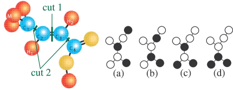
Figure 3: Left: Cutting the graph of chemical bonds (fastest interactions) for the trans-crotonic acid into connected subgraphs. The minimal value of $s$ equals $1/2$. Right: Permuting values stored in spin-$1/2$ nuclei used in quantum computation.

Suppose we want to realize permutation

$$\left(\begin{array}[]{ccccccc}M&C_{1}&H_{1}&C_{2}&C_{3}&H_{2}&C_{4}\\ C_{1}&C_{2}&C_{3}&C_{4}&H_{2}&H_{1}&M\end{array}\right).$$

Following our water and air metaphor discussed previously, the vertices contain $Water$–$Air$–$Water$–$Air$–$Air$–$Air$–$Water$. Once the graph has been cut into the subgraphs as discussed, we turn the entire graph (i.e. container) $90$ degrees clockwise (as illustrated in Figure 3(a)) and observe how the water falls down. First, the vertices $M$ and $C_{1}$ and, at the same time, $C_{2}$ and $C_{3}$, exchange their content leading to $Air$–$Water$–$Air$–$Air$–$Water$–$Water$–$Air$, Figure 3(b). In the second step, the contents of $C_{1}$ and $C_{2}$ and, at the same, time $C_{3}$ and $C_{4}$, are interchanged leading to $Air$–$Air$–$Air$–$Water$–$Water$–$Air$–$Water$, Figure 3(c). Finally, the contents of $C_{2}$ and $C_{3}$ are interchanged leading to $Air$–$Air$–$Air$–$Air$–$Water$–$Water$–$Water$ (Figure 3(d)), meaning that all vertices that were desired in $G_{1}$ are now moved to $G_{1}$, and also all vertices that we wanted to see in $G_{2}$ are now located in $G_{2}$. At this step the problem falls into two completely separate components that can be handled in parallel: permute values in a connected graph with 4 vertices and a connected graph with 3 vertices.

5.3 Implementation and its scalability

We implemented the above algorithms in C++. Our code consists of two major parts one of which is the subcircuit placement, and the second is realization of the swapping algorithm. We next discuss implementation details of each of these parts as well as how they are used to achieve the final placement.

Firstly, we use the VFLib graph matching library [27] to solve graph monomorphism problem which is a basis for the subcircuit placement. The bottleneck of the entire implementation is the efficiency of computing a solution to the subgraph monomorphism problem. This is because in order to solve the placement problem for a circuit with $k$ gates, among which $s$ are two-qubit gates (obviously, $s<k$), the subgraph monomorphism routine is called at most $2s$ times. All other operations performed by our algorithm and its implementation are at most quadratic in $k$.

The efficiency of the VFLib graph matching implementation was studied in [4]. The authors of [4] indicate that the implementation is sufficiently fast for alignment of graphs containing up to 1000 (and sometimes up to 10,000) nodes. A study of runtime for aligning a particular type of graphs with around 1000 vertices showed that the alignment took close to one second on average [4]. We thus conclude that our implementation should not take more than an hour (3600 seconds, in other words, 3600 calls to the subgraph isomorphism subroutine) to place quantum circuits built on a few hundred qubits and containing a few thousand gates.

Our basic implementation of the swapping algorithm is exactly as described in Subsection 5.2, with the communication channel available for a qubit state transfer at any time. We modified this algorithm by adding a heuristic called the leaf–target value override. This heuristic works by inspecting leaf values at every stage of the swapping algorithm, and if a desirable value (according to the final permutation that needs to be realized) can be swapped directly into a vertex of the physical environment that is a leaf, this operation is performed. This leaf with the desired value stored in it is then excluded from the remainder of the swapping algorithm. The set of leaves of the physical environment graph that still participate in the algorithm (because they do not yet contain their target value) is updated dynamically. In practice, this update to the swapping algorithm helped to reduce the depth of the swapping stage on the order of 0-5%.

After each mapping is calculated by our monomorphism routine, we greedily select the least cost mapping. To improve this greedy solution, we added a depth-2 look ahead algorithm that combines the cost of a potential mapping with the associated swap cost and all of the potential next stage mappings and swap costs. The algorithm works as follows.

Given a subcircuit of a maximal size such that it can be placed as a whole we use the VFLib graph monomorphism routine to come up with monomorphisms $M_{1},M_{2},\ldots,M_{k}$ for some fixed value $k$. For each monomorphism, we construct the swappings $S_{1},S_{2},\ldots,S_{k}$ and look for the next monomorphism, followed by the next swapping stage. At this point we have examined $k^{2}$ circuits $M_{1}S_{1}M_{1,1}S_{1,1},\;M_{1}S_{1}M_{1,2}S_{1,2},...,$ $M_{1}S_{1}M_{1,k}S_{1,k},\;M_{2}S_{2}M_{2,1}S_{2,1},\;M_{2}S_{2}M_{2,2}S_{2,2},...,$ $M_{2}S_{2}M_{2,k}S_{2,k},$ $...,M_{k}S_{k}M_{k,k}S_{k,k}$ (only the current best circuit is actually stored) with runtime costs $C_{1,1},\;C_{1,2},...,C_{k,k}$. We choose a minimal value $C_{i,j}$ corresponding to the partial placement $M_{i}S_{i}M_{i,j}S_{i,j}$ and accept matching $M_{i}$ followed by the swapping $S_{i}$. The process is iterated until the entire circuit is placed. In our implementation, we used $k=100$ to limit the number of possible monomorphisms considered. Let us note that the number of times a monomorphism needs to be called is only $2k$ as opposed to the expected $k^{2}$. This is because the sets of monomorphisms $\{M_{i,j}|j=1..n\}$ for different values $i$ are equal.

6 Experimental results

In the experiments described below we modify the circuit depth calculation to take into account that it is not necessary to use an existing interaction more than three times to realize any two-qubit unitary [26]. This means that the cost calculation may be slightly (with the examples we tried, no more than 1%) lower than it would be if the above was not applied.

Table 2: Mapping experimentally constructed circuits into their physical environment.

Circuit			Environment		Estimated	Search
name	# gates	# qubits	name	# qubits	circuit runtime	space size
error correction encoding	9	3	acetyl chloride	3	.0136 sec	6
[14], Figure 2			[14], Figure 1
5 bit error correction	25	5	trans-crotonic	7	.0779 sec	2,520
([12], Fig. 1)			acid ([12], Fig. 3)
pseudo-cat state	54	10	histidine	12	.5170 sec	239,500,800
preparation ([20], Fig. 1)			([20], Fig. 2)

In this section we present three types of experiments. First, we take circuits that were executed experimentally on an existing hardware. We erase the placement assignment of the circuit qubits into the physical environment and try to reconstruct it. Our tool finds the best solutions found by hand by experimentalists (meaning the tool creates only one workspace and the matching made is equivalent to that by experimentalists). Table 2 summarizes the results. The first three columns list properties of the circuit—a short description of what the circuits does and its source, the number of gates and qubits in it. The next two columns present properties of the environment—the name of the environment and its source, and the maximal number of qubits it supports. The Estimated circuit runtime column shows a result of the running time our algorithm formulated—an estimate (actual runtime, depending on the particulars of technology, may be slightly different to account for the second order effects) of how long it will take to execute a given circuit. We do not list the actual mapping, because it is equivalent to that by the experimentalists [12, 14, 20]. The last column presents the size of the search space for placing a circuit as a whole (considering $k$ subcircuits results in power $k$ blow up of the search space size). This tests the quality of our approach via comparison to the known results and it illustrates that our tool correctly chooses to consider only a single subcircuit and places it optimally.

We next describe an extended test in which we considered small but potentially useful computations. These included the following quantum circuits: phase estimation (a 5-qubit “phaseest” circuit), 6-qubit Quantum Fourier Transformation (QFT) circuit ([21], page 219; circuit name “qft6”), 9-qubit approximate QFT (circuit name “aqft9”), 10-qubit $[[7,1,3]]$ Steane code X-type error correction (circuit names “steane-x/z1” and “steane-x/z2”, corresponding to Fig. 10.16 and 10.17 in [21]), which, by symmetry and properties of the circuit, can be thought of as a Z-type error correction, and an approximate 12-qubit QFT (circuit name “aqft12”). Also included in the experiment were the existing liquid state NMR molecules with the most qubits whose complete description we were able to find in the literature. The molecules include a 5-qubit BOC-(¹³C₂-¹⁵N-²D${}_{2}^{\alpha}$-glycine)-fluoride [16], 5-qubit pentafluorobutadienyl cyclopentadienyldicarbonyliron [24], 7-qubit trans-crotonic acid [12], and 12-qubit histidine [20]. Note that the latter two molecules are more recent and the experiments with them were done on better equipment. Thus, it is natural to expect more qubits and a faster associated circuit runtime. In particular, the experiment with pentafluorobutadienyl cyclopentadienyldicarbonyliron is so “slow” that the choice of parameter $Threshold$ equal 50 or 100 disallows all interactions in the molecule making the corresponding computation impossible to run (which is indicated with N/A in Table 3). This test illustrates the importance of using the swapping stages, studies the relation between the value of $Threshold$ and the total circuit runtime, shows the quality of the results, and provides a potentially useful data set for experiments.

The results are formulated in Table 3. Each entry in this table consists of two numbers. The first number shows the calculated total runtime of the placed circuit in the given table row for the $Threshold$ value as declared in the given column, for each physical environment described on top of the given part of the Table. The second entry of the cell is a natural number in brackets that represents how many subcircuits our software chooses to do the placement with. Note, that the last column in Table 3 lists circuit runtime with the optimal placement when placed without insertion of SWAPs. Every number in the row smaller than the last number in it is an indication that our swapping strategy outperformed optimal placement of the circuit as a whole.

In particular, as a part of the analysis of the results in Table 3 let us consider the circuit for a 6 qubit QFT and map it into the 7-qubit trans-crotonic acid molecule. This circuit is inconvenient for quantum architectures since it contains a 2-qubit gate for every pair of qubits. It cannot be executed in a chain nearest neighbor sub-architecture [7] since the longest spin chain in trans-crotonic acid has only five qubits. As expected, usage of a large $Threshold$ value equal to 10000 results in a single working space, with the runtime of the placed circuit decreasing when reducing the value of $Threshold$. However, the number of individually aligned subcircuits grows, and, as a result, the time spent in swapping the values increases. For a very low $Threshold$ value equal to $50$ (in this case, the adjacency graph of the molecule is disconnected, which, in fact, is an indication that the value of $Threshold$ is already too small to give the best placement result), the mapped circuit does too much swapping, resulting in a high overall cost. The best result is achieved with $Threshold=200$. This indicates that the quantum circuit placement tool has to use some rounds of SWAPs to achieve best results. This is because the circuit with $Threshold$ value 10000 is placed optimally as whole (i.e. when no SWAPs are allowed). The best circuit execution time with a “smart” multiple-subcircuit placement that we were able to achieve is $.2237$ sec. This is almost twice as fast as $.4137$ sec, which is the best one can possibly achieve by placing the circuit as a whole. A more dramatic change in the circuit runtime when considering subcircuits can be observed with the circuits “phaseest” and “steane-x/z”.

Table 3: Placement of potentially interesting circuits in the existing physical environments for different values of the $Threshold$.

Placement with the 5-qubit BOC-(13C2-15N-2D${}_{2}^{\alpha}$-glycine)-fluoride molecule [16]
Circuit	Threshold
	50	100	200	500	1000	10000
phaseest	.9980 sec (8)	.9980 sec (8)	.8167 sec (4)	.8167 sec (4)	.4314 sec (3)	.5632 sec (1)
Placement with the 5-qubit pentafluorobutadienyl cyclopentadienyldicarbonyliron molecule [24]
Circuit	Threshold
	50	100	200	500	1000	10000
phaseest	N/A	N/A	8.2092 sec (8)	7.7179 sec (4)	7.7179 sec (4)	.3733 sec (1)
Placement with the 7-qubit trans-crotonic acid [12]
Circuit	Threshold
	50	100	200	500	1000	10000
phaseest	.1636 sec (7)	.0699 sec (4)	.0699 sec (4)	.0700 sec (3)	.2156 sec (2)	.1812 sec (1)
qft6	.3766 sec (9)	.3294 sec (5)	.2237 sec (5)	.2308 sec (5)	.3120 sec (3)	.4137 sec (1)
Placement with the 12-qubit histidine molecule [20]
Circuit	Threshold
	50	100	200	500	1000	10000
phaseest	1.2022 sec (7)	.6860 sec (4)	.6860 sec (4)	.1827 sec (3)	.1517 sec (2)	.1870 sec (1)
qft6	1.9824 drv (9)	.9519 sec (6)	1.1607 sec (5)	.3123 sec (4)	.5623 sec (3)	.4412 sec (1)
aqft9	4.3713 sec (15)	2.5419 sec (10)	1.3405 sec (8)	1.5400 sec (7)	1.4927 sec (4)	1.3367 sec (1)
steane-x/z1	1.7427 sec (10)	1.1898 sec (4)	1.3402 sec (4)	1.6326 sec (4)	.5990 sec (2)	1.0436 sec (1)
steane-x/z2	1.3233 sec (7)	1.2715 sec (4)	1.0110 sec (3)	.4166 sec (2)	.4677 sec (2)	.9515 sec (1)
aqft12	8.1046 sec (23)	5.3014 sec (15)	6.0413 sec (13)	3.5143 sec (10)	3.3362 sec (8)	2.6426 sec (1)

In the final experiment, we test the performance and scalability of our implementation. We begin by generating physical environments for the test with $N$ qubits, $x_{1},x_{2},\ldots,x_{N}$, that form a linear nearest neighbor architecture. The interaction time between a pair of neighboring qubits is set to the value $.001$ sec per a 90-degree 2-qubit rotation (one can think of it as a 1 KHz quantum processor). Such an architecture seems very natural given the efforts in the experimental implementation of the linear nearest neighbor architectures [19].

When constructing the test circuit we first randomly permute qubits into $p_{1},p_{2},\ldots,p_{N}$ where $p_{j}=x_{i},1\leq j\leq N$, $1\leq i\leq N$. We use this permutation to represent a chain architecture where any qubit $p_{j}$ is coupled to qubits $p_{j-1}$ and $p_{j+1}$. We then generate a random circuit for execution over this physical environment with $N$ qubits and $N\times\log^{2}(N)$ gates (we assume gates have maximal “length”, i.e. $T(G)=3$ [26]). We do this by first generating gates by randomly choosing an index $j$ and create a two-qubit gate between $p_{j}$ and $p_{j-1}$ or $p_{j}$ and $p_{j+1}$, each with probability $1/2$. After $N\times\log(N)$ gates are created, we again randomly permute our $N$ elements and then randomly generate $N\times\log(N)$ gates in the chain nearest neighbor architecture that corresponds to this permutation. This is repeated $\log(N)$ times. We refer to each of these permutations as “hidden stages”. The reason behind constructing such a test circuit is as follows. Some quantum computations are likely to consist of a number of fairly short phases that are developed and optimized separately, and then need to be “glued” together to compose the desired computation. For instance, Shor’s factoring algorithm [22] consists of modular exponentiation and quantum Fourier transformation circuits (approximate QFT circuits have $O(N\times\log(N))$ gates), each studied as a separate problem in the relevant literature (for example, [18, 17]); modular exponentiation itself can be broken into a number of simpler arithmetic circuits.

Table 4 displays the results of this experiment for values of $N=8$ up to $N=1024$. The first column is the number of qubits used in each experiment, the second column is the number of gates, and the third is the number of “hidden stages”, i.e. the number of random permutations used while generating the circuit’s description. The fourth column is the number of subcircuits generated by our implementation during placement. This column exactly corresponds to the number of hidden stages, which was expected, as we must have a swapping stage to move our temporary architecture from one permutation to the next. The fifth column is the quantum circuit runtime as computed by our placement algorithm and the final column is the running time of our software (user time) to compute the placement. The results in Table 4 indicate that our implementation can process large (hundreds of qubits, tens of thousands gates) circuits in reasonable time and come up with a sensible placement. We used an Athlon 64 X2 3800+ machine with 2 GB RAM memory running Linux 2.6.20 for all our experiments.

Table 4: Performance test for circuit placement over chains.

# of Qubits	# of Gates	Hidden Stages	# of Subcircuits	Circuit Runtime	Software Runtime
8	72	3	3	.118 sec	0.02 sec
16	256	4	4	.458 sec	0.12 sec
32	800	5	5	.937 sec	1.34 sec
64	2304	6	6	2.747 sec	7.52 sec
128	6272	7	7	7.147 sec	69.63 sec
256	16384	8	8	16.88 sec	674.96 sec
512	41472	9	9	38.107 sec	9328.00 sec
1024	102400	10	10	86.2820 sec	173296.00 sec

7 Conclusions

In this paper we considered the problem of the efficient assignment of physical qubits to logical qubits in a given circuit, referred to as placement. We studied theoretical aspects of the problem and proved that even a simplified place-all-at-once version of the placement problem is NP-Complete. We thus concentrated on a heuristic solution. We presented an algorithm for the quantum circuit placement problem and its implementation. We tested our software on experimental data and computed, within a fraction of a second, the best results that have been reported by the experimental physicists. Further analysis indicates that our tool can handle very large quantum circuits (hundreds of qubits and thousands of gates) in a reasonable time (hours), and it is efficient. We found that considering subcircuits and swapping their mappings is essential in achieving the best placement results.

Further research may be done in the direction of finding a good balance between the depth of a useful computation and the depth of the following swapping stage (right now, our method is greedy in that the computational stage is formed to be as large as possible), and using gate commutation (more generally, circuit identities) to transform an instance of the circuit placement problem into a possibly more favorable one.

Appendix

Theorem 1.

Every bounded degree graph of maximal degree $k$ is well separable with parameter $s=\frac{1}{k}$.

Proof.

In our proof we start with a small connected subgraph $G_{1}$ such that the graph $\hat{G_{1}}$ that complements it to $G$ is itself connected and iteratively add more vertices to it until at some step $t$ the resulting graph $G_{t}$ contains at least $\frac{n-1}{k}$ and at most $n-\frac{n-1}{k}$ vertices, while its complement to $G$ stays connected.

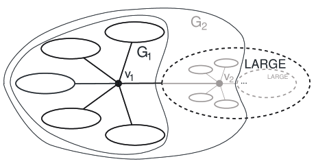
Figure 4: Finding a connected component with at least $\frac{n-1}{k}$ and at most $n-\frac{n-1}{k}$ vertices, whose complement to $G$ is also a connected graph.

Consider vertex $v_{1}\in G$ whose degree $\deg(v_{1})\leq k$. Cut some edges of $G$ until it becomes a tree, but do so without touching edges connected to $v_{1}$. Each of the ellipses illustrated in Figure 4 in black color is now a connected tree. If one of them, say $i^{\textrm{th}}$, contains at least $\frac{n-1}{k}$ and at most $n-\frac{n-1}{k}$ vertices, cut the edge leading to this subtree and the entire graph breaks into two connected components, $G_{t}$ and its complement. At this point, each of the components can be processed iteratively to achieve well separability. In the case when a component with at least $\frac{n-1}{k}$ and at most $n-\frac{n-1}{k}$ vertices does not exist, the only possibility is to have one large component having more than $n-\frac{n-1}{k}$ vertices, and a number of small components. Suppose the edge that joins $v_{1}$ and large component is $(v_{1},v_{2})$. Unite all small components into a graph that we will further refer to as $G_{1}$. $G_{1}$ contains at least $\deg(v_{1})$ vertices.

Vertex $v_{2}$ is connected to $G_{1}$ and $\deg(v_{2})-1$ other connected components. If among other components there exists one with at least $\frac{n-1}{k}$ and at most $n-\frac{n-1}{k}$ vertices, we have found what we were looking for. Otherwise, there exists one large (with at least $n-\frac{n-1}{k}$ vertices) component and a number of small ones. In such case, we join $G_{1}$ with these components such as shown in Figure 4 and call this graph $G_{2}$. Graph $G_{2}$ has at least one more vertex than $G_{1}$, because $v_{2}$ is in $G_{2}$ but not in $G_{1}$. Continue this process with vertices $v_{3}$, $v_{4}$, and so on until we accumulated at least $\frac{n-1}{k}$ vertices in the smaller component or until we found such component otherwise.

It might not be possible to always find a connected component with strictly more than $\frac{n-1}{k}$ and strictly less than $n-\frac{n-1}{k}$ components, because in the worst case scenario we may have a vertex $v$ of degree exactly $k$ such that it is connected to pairwise disconnected graphs with exactly $\frac{n-1}{k}$ vertices each. Then, the best we can do is separate one such component from the remainder of the graph, which will result in the construction of two connected components with $\frac{n-1}{k}$ and $n-\frac{n-1}{k}$ vertices each. The relation between the number of vertices in such graphs is

$$\frac{\frac{n-1}{k}}{n-\frac{n-1}{k}}=\frac{n-1}{nk-n+1}\geq\frac{n-1}{nk-k}=\frac{1}{k}.$$

∎

References

- [1] D. Aharonov and M. Ben-Or. Fault-tolerant quantum computation with constant error. Proceedings of ACM STOC, pages 176–188, 1997.
- [2] M. D. Bowdrey, J. A. Jones, E. Knill, and R. Laflamme. Compiling gate networks on an Ising quantum computer. Physical Review A, 72(032315), 2005, quant-ph/0506006.
- [3] D. Copsey, M. Oskin, F. Impens, T. Metodiev, A. Cross, F. T. Chong, I. L. Chuang, and J. Kubiatowicz. Toward a scalable silicon-based quantum computing architecture. IEEE Journal of Selected Topics in Quantum Electronics, 9(6):1552--1569, 2003.
- [4] L. P. Cordella, P. Foggia, C. Sansone, and M. Vento. Performance evaluation of the VF graph matching algorithm. 10th ICIAP, vol. 2, pages 1038--1041, 1999.
- [5] D. G. Cory, R. Laflamme, E. Knill, L. Viola, T.F. Havel, N. Boulant, G. Boutis, E. Fortunato, S. Lloyd, R. Martinez, C. Negrevergne, M. Pravia, Y. Sharf, G. Teklemariam, Y. S. Weinstein, and W.H. Zurek. NMR based quantum information processing: achievements and prospects. quant-ph/0004104, April 2000.
- [6] H. K. Cummins, C. Jones, A. Furze, N. F. Soffe, M. Mosca, J. M. Peach, J. A. Jones. Approximate quantum cloning with nuclear magnetic resonance. Physical Review Letters, 88:187901, 2002, quant-ph/0111098.
- [7] A. G. Fowler, S. J. Devitt, and L. C. L. Hollenberg. Implementation of Shor’s algorithm on a linear nearest neighbor qubit array. Quantum Information and Computation, 4(4):237--251, 2004, quant-ph/0402196.
- [8] M. R. Geller, E. J. Pritchett, A. T. Sornborger, F. K. Wilhelm. Quantum computing with superconductors I: Architectures. March 2006, quant-ph/0603224.
- [9] H. Häffner, W. Hänsel, C. F. Roos, J. Benhelm, D. Chek-al-kar, M. Chwalla, T. Körber, U. D. Rapol, M. Riebe, P. O. Schmidt, C. Becher, O. Gühne, W. Dür, and R. Blatt. Scalable multiparticle entanglement of trapped ions. Nature 438:643--646, December 2005, quant-ph/0603217.
- [10] R. Hughes et al. Quantum Computation Roadmap, July 2004. http://qist.lanl.gov/qcomp map.shtml
- [11] J. A. Jones. NMR quantum computation: a critical evaluation. Fortschr. Phys. 48(9-11):909--924, 2000, quant-ph/0002085.
- [12] E. Knill, R. Laflamme, R. Martinez, and C. Negrevergne. Implementation of the five qubit error correction benchmark. Physical Review Letters, 86(5811), 2001, quant-ph/0101034.
- [13] E. Knill, R. Laflamme, R. Martinez, and C.-H. Tseng. An algorithmic benchmark for quantum information processing. Nature, 404:368--370, March 2000.
- [14] M. Laforest, D. Simon, J.-C. Boileau, J. Baugh, M. Ditty, and R. Laflamme. Using error correction to determine the noise model. Physical Review A 75(012331), 2007, quant-ph/0610038.
- [15] L. Lavagno, G. Martin, and L. Scheffer, editors. Electronic Design Automation for Integrated Circuits Handbook. CRC Taylor and Francis, 2006.
- [16] R. Marx, A. F. Fahmy, J. M. Myers, W. Bermel, and S. J. Glaser. Realization of a 5-bit NMR Quantum Computer Using a New Molecular Architecture. May 1999, quant-ph/9905087.
- [17] D. Maslov. Linear Depth Stabilizer and Quantum Fourier Transformation Circuits with no Auxiliary Qubits in Finite Neighbor Quantum Architectures. Physical Review A, 2007, quant-ph/0703211.
- [18] R. Van Meter and K. M. Itoh. Fast quantum modular exponentiation. Physical Review A, 71(052320), May 2005, quant-ph/0408006.
- [19] R. Van Meter and M. Oskin. Architectural implications of quantum computing technologies. ACM Journal on Emerging Technologies in Computing Systems, 2(1):31--63, 2006.
- [20] C. Negrevergne, T. S. Mahesh, C. A. Ryan, M. Ditty, F. Cyr-Racine, W. Power, N. Boulant, T. Havel, D. G. Cory, and R. Laflamme. Benchmarking quantum control methods on a 12-qubit system. Physical Review Letters, 96(170501), 2006, quant-ph/0603248.
- [21] M. Nielsen and I. Chuang. Quantum Computation and Quantum Information. Cambridge University Press, 2000.
- [22] P. W. Shor. Polynomial-time algorithms for prime factorization and discrete logarithms on a quantum computer. SIAM Journal of Computing, 26:1484--1509, 1997, quant-ph/9508027.
- [23] A. Skinner, M. Davenport, and B. Kane. Hydrogenic spin quantum computing in silicon: a digital approach. Physical Review Letters, 90(087901), 2003, quant-ph/0206159.
- [24] L. M. K. Vandersypen, M. Steffen, G. Breyta, C. S. Yannoni, R. Cleve, and I. L. Chuang. Experimental Realization of an Order-Finding Algorithm with an NMR Quantum Computer. Physical Review Letters 85(25):5452-5455, December 2000, quant-ph/0007017.
- [25] M. Whitney, N. Isailovic, Y. Patel, J. Kubiatowicz. Automated Generation of Layout and Control for Quantum Circuits. April 2007, arXiv:0704.0268v1.
- [26] J. Zhang, J. Vala, S. Sastry, and K. B. Whaley. Geometric theory of nonlocal two-qubit operations. Physical Review A, 67(042313), 2003, quant-ph/0209120.
- [27] Intelligent Systems and Artificial Vision Lab. The VFLib graph matching library. http://amalfi.dis.unina.it/graph/, 2006.