Decoherence of an $n$-qubit quantum memory

Abstract

We analyze decoherence of a quantum register in the absence of non-local operations i.e. of $n$ non-interacting qubits coupled to an environment. The problem is solved in terms of a sum rule which implies linear scaling in the number of qubits. Each term involves a single qubit and its entanglement with the remaining ones. Two conditions are essential: first decoherence must be small and second the coupling of different qubits must be uncorrelated in the interaction picture. We apply the result to a random matrix model, and illustrate its reach considering a GHZ state coupled to a spin bath.

Physical devices capable of storing faithfully a quantum state, i.e. quantum memories, are crucial for any quantum information task. While different types of systems have been considered, most of the effort is concentrated in manipulating qubits as they are essential for most quantum information tasks Nielsen and Chuang (2000). For a general quantum memory (QM) it is necessary to record, store and retrieve an arbitrary state. For quantum communication and quantum computation initialization in the base state, single qubit manipulations, a two qubit gate (e.g. control-not), and single qubit measurements are sufficient. For arbitrary quantum memories recording and retrieving the state is still an experimental challenge but initializing a qubit register and individual measurement is mostly mastered. Faithful realization of two qubit gates together with better isolation from the environment are the remaining obstacles for achieving fully operational quantum technology. However the huge effort done in the community has born some fruit A. Poppe et al. (2004); qme .

A number of papers discuss how two qubit quantum memories are affected by coupling to some environment. In our previous work we study the case of two qubits interacting either with a spin bath Pineda and Seligman (2006) or a random matrix environment Pineda and Seligman (2007); Pineda et al. (2006). In both cases the loss of coherence and the loss of internal entanglement of the pair was studied. Many other papers focus on the loss of internal entanglement only, due to the interaction with a thermal bath (see Mintert et al. (2005) and references therein). A study of decoherence of a two-qubit system as measured by entanglement fidelity is presented in K. Surmacz et al. (2006). There the effect of fluctuations of the parameters of the Hamiltonian is analyzed. In Massimo Palma et al. (1996); Reina et al. (2002) an $n$ qubit QM coupled to a bath of harmonic oscillators is studied.

In the present letter we give analytic expressions for the decoherence of a QM during the storage time. Specifically we discuss a QM composed of a set of individual qubits interacting with an environment. The expressions given are based on previous knowledge of the decoherence of a single qubit entangled with some spectator, with which it does not interact. Their validity is limited to small decoherence, i.e. large purity of the QM. Note that the latter is no significant restriction due to the high fidelity requirements for the application of quantum error correction codes. We assume that the entire system is subject to unitary time-evolution, and that decoherence comes about by entanglement between the central system and the environment. Because of its simple analytical structure decoherence shall be measured in terms of purity Zurek (1991) of the central system. Spurious interactions inside the central system are neglected. We shall rely heavily on our recent studies of decoherence of two qubits Pineda and Seligman (2007); Pineda et al. (2006).

A further and critical assumption is the independence of the coupling in the interaction picture. This is justified if the couplings are independent in the Schrödinger picture or if we have rapidly decaying correlations due to mixing properties of the environment in the spirit of Prosen and Seligman (2002). Physically the first would be more likely if we talk about qubits realized in different systems or degrees of freedom, while the second seems plausible for many typical environments.

We generalize the concept of a spectator configuration Pineda and Seligman (2006, 2007); Pineda et al. (2006): The central system consists of two non-interacting parts, one interacting with the environment and the other not. This configuration is non-trivial if the two parts of the central system are entangled. In our case the first part will be a single qubit and the second part (the spectator) will consist of all other qubits of the QM. Our central result is then a decomposition of the decoherence of the full QM, as measured by purity, in a sum of terms describing the decoherence of each qubit in a spectator configuration. Apart from the above made assumptions, this result does not depend on any particular property of the environment or the coupling. Thus it can be applied to a variety of models.

We test successfully the results in a random matrix model both for coupling and bath Pineda and Seligman (2007); Pineda et al. (2006). The general relation is obtained in linear response approximation and leads to explicit analytic results if the spectral correlations of the bath are known. Finally, we perform numerical simulations for two and four qubits, interacting with a kicked Ising spin chain Pineda and Seligman (2006); Prosen (2002); Pineda and Prosen (2007) as an environment, which can be chosen mixing or integrable.

The central system (our QM) is composed of $n$ qubits. Thus its Hilbert space is $\mathcal{H}_{\mathrm{qm}}=\bigotimes_{i=1}^{n}\mathcal{H}_{i}$, where $\mathcal{H}_{i}$ are the Hilbert spaces of the qubits ($\dim\mathcal{H}_{i}=2$). The Hilbert space of the environment is denoted by $\mathcal{H}_{\mathrm{e}}$. The Hamiltonian reads as

$$H=H_{\mathrm{qm}}+H_{\mathrm{e}}+\lambda V\;.$$ (1)

Here, $H_{\mathrm{qm}}=\sum_{i=1}^{n}H_{i}$, where $H_{i}$ acts on $\mathcal{H}_{i}$, whereas $H_{\mathrm{e}}$ describes the dynamics of the environment and

$$\lambda V=\sum_{i=1}^{n}\lambda_{i}V^{(i)}$$ (2)

the coupling of the qubits to the environment. The strength of the coupling of qubit $i$ is controlled by the parameter $\lambda_{i}$, while $\lambda=\max\{|\lambda_{i}|\}$.

We consider two different settings. In the first one $V^{(i)}$ acts on the space $\mathcal{H}_{i}\otimes\mathcal{H}_{\mathrm{e}}$, i.e. all qubits interact with a common environment. We shall name this the joint environment configuration. In the second one each qubit interacts with a separate environment. Thus the environment is split into $n$ parts, $\mathcal{H}_{\mathrm{e}}=\bigotimes_{i=1}^{n}\mathcal{H}_{\mathrm{e},i}$ and $V^{(i)}$, in eq. (2), acts only on $\mathcal{H}_{i}\otimes\mathcal{H}_{\mathrm{e},i}$. This we call the separate environment configuration. The first case would be typical for a quantum computer, where all qubits are close two each other, while the second would apply to a non-local quantum network.

We choose the initial state to be the product of a pure state of the central system (the QM) and a pure state of the environment. It may be written as

$$|\psi_{0}\rangle=|\psi_{\mathrm{qm}}\rangle|\psi_{\mathrm{e}}\rangle,\quad|\psi_{\mathrm{qm}}\rangle\in\mathcal{H}_{\mathrm{qm}},\,|\psi_{\mathrm{e}}\rangle\in\mathcal{H}_{\mathrm{e}}.$$ (3)

Thus, the reduced initial state in the quantum memory $\varrho_{0}=\mathop{\mathrm{tr}}\nolimits_{\mathrm{e}}|\psi_{0}\rangle\langle\psi_{0}|=|\psi_{\mathrm{qm}}\rangle\langle\psi_{\mathrm{qm}}|$ is pure. In the separate environment configuration we furthermore assume that $|\psi_{\mathrm{e}}\rangle=\bigotimes_{i}|\psi_{\mathrm{e},i}\rangle$ with $|\psi_{\mathrm{e},i}\rangle\in\mathcal{H}_{\mathrm{e},i}$, which corresponds to the absence of quantum correlations among the different environments.

For reasons of analytic simplicity we chose the purity $P(t)$ as measure for decoherence. It is defined as

$$P(t)=\mathop{\mathrm{Tr}}\nolimits\rho_{\mathrm{qm}}^{2}(t),\;\rho_{\mathrm{qm}}(t)=\mathop{\mathrm{Tr}}\nolimits_{\mathrm{e}}\mathrm{e}^{-\imath Ht}|\psi_{0}\rangle\langle\psi_{0}|\mathrm{e}^{\imath Ht}.$$ (4)

To calculate purity or any other measure of decoherence we can replace the forward time evolution $\exp(-\imath Ht)$ by the echo operator $M(t)=\exp(\imath H_{0}t)\,\exp(-\imath Ht)$ where $H_{0}$ determines the evolution without coupling ($\lambda=0$). In linear response approximation this operator reads as

$$M(t)=\openone-\imath\lambda I(t)-\lambda^{2}J(t),$$ (5)

where $I(t)=\int_{0}^{t}\mathrm{d}\tau\tilde{V}_{\tau}$ and $J(t)=\int_{0}^{t}\mathrm{d}\tau\int_{0}^{\tau}\mathrm{d}\tau^{\prime}\tilde{V}_{\tau}\tilde{V}_{\tau^{\prime}}$. $\lambda\tilde{V}_{t}=\exp(\imath H_{0}t)\,\lambda V\exp(-\imath H_{0}t)$ is the coupling at time $t$ in the interaction picture. As discussed in Pineda et al. (2006) it is convenient to introduce the form $p[\rho_{1}\otimes\rho_{2}]=\mathop{\mathrm{Tr}}\nolimits(\mathop{\mathrm{Tr}}\nolimits_{\mathrm{e}}\rho_{1}\mathop{\mathrm{Tr}}\nolimits_{\mathrm{e}}\rho_{2})$. Purity is then given by

$$P(t)=1-2\lambda^{2}\int_{0}^{t}\mathrm{d}\tau\int_{0}^{t}\mathrm{d}\tau^{\prime}{\rm Re}\,A(\tau,\tau^{\prime})+\mathord{\mathrm{O}}\left(\lambda^{3}\right)$$ (6)

with

$$A(\tau,\tau^{\prime})=p[\tilde{V}_{\tau}\tilde{V}_{\tau^{\prime}}\varrho_{0}\otimes\varrho_{0}]-p[\tilde{V}_{\tau^{\prime}}\varrho_{0}\tilde{V}_{\tau}\otimes\varrho_{0}]\\ +p[\tilde{V}_{\tau}\varrho_{0}\otimes\tilde{V}_{\tau^{\prime}}\varrho_{0}]-p[\tilde{V}_{\tau^{\prime}}\varrho_{0}\otimes\varrho_{0}\tilde{V}_{\tau}]\;.$$ (7)

Note that the linear terms vanish after tracing out the environment. Considering the form of the coupling in Eq. (2) we can decompose $\lambda^{2}A(\tau,\tau^{\prime})=\sum_{i,j}\lambda_{i}\lambda_{j}A^{(i,j)}(\tau,\tau^{\prime})$ with

$$A^{(i,j)}(\tau,\tau^{\prime})=p[\tilde{V}^{(i)}_{\tau}\tilde{V}^{(j)}_{\tau^{\prime}}\varrho_{0}\otimes\varrho_{0}]-p[\tilde{V}^{(i)}_{\tau^{\prime}}\varrho_{0}\tilde{V}^{(j)}_{\tau}\otimes\varrho_{i}]\\ +p[\tilde{V}^{(i)}_{\tau}\varrho_{0}\otimes\tilde{V}^{(j)}_{\tau^{\prime}}\varrho_{0}]-p[\tilde{V}^{(i)}_{\tau^{\prime}}\varrho_{0}\otimes\varrho_{0}\tilde{V}^{(j)}_{\tau}]\;.$$ (8)

$\tilde{V}^{(i)}_{t}=\exp(\imath H_{0}t)\,V^{(i)}\exp(-\imath H_{0}t)$ in analogy with $\tilde{V}_{t}$. Equation (6) is then given as a double sum in the indices of the qubits. In the diagonal approximation ($i=j$), $P(t)$ can be expressed in terms of purities $P^{(i)}_{\rm(sp)}(t)$ associated with individual qubits

$$P(t) = 1-\sum_{i=1}^{n}\left(1-P^{(i)}_{\rm(sp)}(t)\right),$$ (9)

$$P^{(i)}_{\rm(sp)}(t) = 1-2\lambda_{i}^{2}\int_{0}^{t}\mathrm{d}\tau\int_{0}^{t}\mathrm{d}\tau^{\prime}A^{(i,i)}(\tau,\tau^{\prime})+\mathord{\mathrm{O}}\left(\lambda_{i}^{3}\right).$$

Each contribution corresponds to the purity decay of the central system in a spectator configuration with qubit $i$ interacting with the environment. Eq. (9) is the central result of this paper. The diagonal approximation is justified in two situations: First if the couplings $V^{(i)}$ of the individual qubits are independent from the outset, as would be typical for the separate environment configuration or for the random matrix model of decoherence Pineda et al. (2006). Second, if the couplings in the interaction picture become independent due to mixing properties of the environment, as would be typical for a “quantum chaotic” environment.

To illustrate the case of independent couplings mentioned above, random matrix theory provides a handy example. Such models were discussed in Gorin and Seligman (2002); Pineda and Seligman (2007); Abreu and Vallejos (2007) and describe the couplings $V^{(i)}$ by independent random matrices, chosen from the classical ensembles cla .

In Pineda et al. (2006); Pineda and Seligman (2007) the purity decay was computed in linear response approximation for two qubits, one of them being the spectator. For the sake of simplicity we choose the joint environment configuration, no internal dynamics for the qubits, and let $H_{\mathrm{e}}$ and $V^{(1)}$ be typical members of the Gaussian unitary ensemble. Purity is then given by

$$P^{(1)}_{\rm(sp)}(t) = 1-\lambda_{1}^{2}(2-p_{1})f(t);$$ (10)

$$f(t) = t\,\max\{t,\tau_{H}\}+\frac{2}{3\tau_{H}}\,\min\{t,\tau_{H}\}^{3}.$$ (11)

Here, $\tau_{H}$ is the Heisenberg time of the environment, and $p_{1}$ is the initial purity of the first qubit alone, which measures its entanglement with the rest of the QM. As we required independence of the couplings, we can now insert eq. (10) in eq. (9) to obtain the simple expression

$$P(t)=1-f(t)\sum_{i=1}^{n}\lambda_{i}^{2}(2-p_{i}),$$ (12)

where $p_{i}$ is the initial purity of qubit $i$. In the presence of internal dynamics the spectator result is also known Pineda et al. (2006) and can be inserted. As an example, we apply the above equation to an initial GHZ state ($(|0\cdots 0\rangle+|1\cdots 1\rangle)/\sqrt{2}$). Then all $p_{i}=1/2$ and we obtain $P(t)=1-(3/2)f(t)\sum_{i}\lambda_{i}^{2}$. For a W state $(|10\ldots 0\rangle+|01\ldots 0\rangle+\cdots+|00\ldots 1\rangle)/\sqrt{n}$, purity for each qubit is $p_{i}=(n^{2}-2n+2)/n^{2}\approx 1$, in the large $n$ limit, and purity decays as $P(t)=1-f(t)\sum_{i}\lambda_{i}^{2}$. For $n=2$ we retrieve the results published in Pineda et al. (2006).

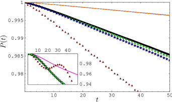
Figure 1: (Color online) Purity decay for a GHZ state is shown for the environment described by eq. (13). The couplings are: all qubits to one spin (red triangles), nearby spins (blue stars), and maximally separated spins (green squares). The theoretical result (thick line) is calculated in terms of the $P^{(i)}_{\rm(sp)}(t)$ (thin lines). The main figure corresponds to the case of a mixing environment and the inset for an integrable one.

The main assumption in Eq. (9) is the fast decay of correlations for couplings of different qubits to the bath. For the random matrix model discussed above this is trivially fulfilled. Yet, integrable environments are commonly used Caldeira and Leggett (1983) and one may wonder whether Eq. (9) can hold in such a context. We shall therefore study a dynamical model where a few qubits are coupled to an environment represented by a kicked Ising spin chain using identical coupling operators for all qubits. In this model, the variation of the angle of the external kicking field allows the transition from a “quantum chaotic” to an integrable Hamiltonian for the environment Prosen (2002). The Hamiltonian of the chain is given by

$$H^{(\mathrm{e})}=\sum_{i=0}^{L-1}\sigma_{x}^{(\mathrm{e},i)}\sigma_{x}^{(\mathrm{e},i+1)}+\boldsymbol{\delta}(t)\sum_{i=0}^{L-1}b\cdot\sigma^{(\mathrm{e},i)}$$ (13)

where $\boldsymbol{\delta}(t)$ is a train of Dirac delta functions at integer times, $L$ is the number of spins in the environment, $\sigma^{(\mathrm{e},i)}=(\sigma_{x}^{(\mathrm{e},i)},\sigma_{y}^{(\mathrm{e},i)},\sigma_{z}^{(\mathrm{e},i)})$ are the Pauli matrices of spin $i$, and $b$ the dimensionless magnetic field with which the chain is kicked ($\hbar=1$). We close the ring requiring $\sigma^{(\mathrm{e},L)}=\sigma^{(\mathrm{e},0)}$. The Hamiltonian of the QM is $H^{(\mathrm{qm})}=\boldsymbol{\delta}(t)\sum_{i}b\cdot\sigma^{(\mathrm{qm},i)}$, where $\sigma^{(\mathrm{qm},i)}$ is defined similarly as for the environment. The coupling is given by $\lambda V=\lambda\sum_{i}\sigma_{x}^{(\mathrm{qm},i)}\sigma_{x}^{(\mathrm{e},j_{i})}$, where the $j_{i}$’s define the positions where the qubits are coupled to the spin chain, e.g. if all $j_{i}$ are equal, all qubits of our QM are coupled to the same position.

To implement a chaotic environment, we use $b=(0.9,0.9,0)$. For these values the quantum-chaos properties have been tested extensively Pineda and Prosen (2007). We use a ring consisting of $L=12$ spins for the environment and $4$ additional spins for the qubits of the QM. The coupling strength has been fixed to $\lambda=0.005$. In Fig. 1, we study purity decay when all four qubits are coupled to the same spin, when they are coupled to neighboring spins, and when they are coupled to maximally separated spins, $\vec{j}=(0,3,6,9)$. The initial state is the product of a GHZ state in the QM and a random pure state in the environment. We compare the results with the prediction of Eq. (9) obtained from simulations of the corresponding spectator configurations (thin solid line). All spectator configurations yield almost the same result for $P(t)$, so that we can see only one line. The figure demonstrates the validity of eq. (9) for well separated and hence independent couplings. For smaller separations we obtain faster decay.

Next we perform similar calculations for integrable environments. A typical case is shown in the inset of fig. 1 for a two qubit QM and $b=(0,1.53,0)$. Both qubits are coupled to the same, neighboring or opposite spins in the ring. Purity decay is faster than in the mixing case as can be expected from general considerations in Gorin et al. (2006). Nevertheless the sum rule is again well fulfilled except if we couple both qubits to the same spin. This leads us to check the behavior of the correlation function

$$p[\tilde{V}^{(i)}_{\tau}\tilde{V}^{(j)}_{\tau^{\prime}}\varrho_{0}\otimes\varrho_{0}]=\langle\psi_{0}|\tilde{V}^{(i)}_{\tau}\tilde{V}^{(j)}_{\tau^{\prime}}|\psi_{0}\rangle.$$ (14)

This is the simplest and usually largest term in $A^{(i,j)}$, eq. (8). Figure 2 shows this quantity for mixing and integrable environments in the first and second row respectively. The first column shows the autocorrelation function ($i=j$). The second and third column give the cross correlation function ($i\neq j$) when the qubits are coupled to the same or opposite spins respectively. We see that in the latter case correlations in both the integrable and the chaotic case are small, thus showing that also in integrable situations our condition can be met. Non-vanishing correlations, as in fig. 2(b) and fig. 2(e) lead to deviations from the sum rule. The pronounced structure for the integrable environment, fig. 2(e), may be associated with the oscillations of purity decay (inset of fig. 1).

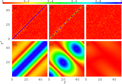
Figure 2: (Color online) The color-coded absolute value of the real part of $\langle\psi_{0}|\tilde{V}^{(i)}_{\tau}\tilde{V}^{(j)}_{\tau^{\prime}}|\psi_{0}\rangle$ given in eq. (14) as a function of $\tau$ and $\tau^{\prime}$ for the integrable [(a) (b) (c)] and the chaotic [(d) (e) (f)] spin chain environment ($L=8$). (a),(d) show the autocorrelation function ($i=j$); (b), (e) and (c) (f) the cross correlation function for couplings to the same spin or opposite spins in the ring respectively.

We have calculated generic decoherence of an $n$-qubit quantum memory as represented by purity decay. For large purities it is globally given in linear response approximation by a sum rule in terms of the purities of the individual qubits entangled with the remaining register as spectator. This sum rule depends crucially on the absence or rapid decay of correlations between the couplings of different qubits in the interaction picture. We prove, that this is fulfilled by sufficiently chaotic environments or couplings, but using a spin chain model as an environment we find, that even if the latter is integrable correlations can be absent and the sum rule holds. While exceptions, no doubt, can be constructed we have a very general tool to reduce the decoherence of a QM of $n$ qubits to the problem of a single qubit entangled with the rest of the QM. Furthermore the result is equally valid if we perform local operations on the qubits. The sum rule also applies if the register is split into arbitrary sets of qubits. In fact one and two qubit gates are known to be universal for quantum computation Nielsen and Chuang (2000), so we lay the foundation for the computation of decoherence during the execution of a general algorithm. This extension only requires the knowledge of the decoherence of a pair suffering the gate operation while entangled with the rest of the register. As each gate is different, we will have to take a step by step approach, which at each step will only involve one and two qubit decoherence. The linear response approximation will be sufficient due to the high fidelity requirements of quantum computation.