Distinguishability of apparatus states in quantum measurement in the Stern-Gerlach experiment

Abstract

In the context of the quantum mechanical modelling of a measurement process using the Stern-Gerlach setup, we critically examine the relationship between the notion of ‘distinguishability’ of apparatus states defined in terms of the inner product and spatial separation among the emerging wave packets. We show that, in general, the mutual orthogonality of these wave packets does not necessarily imply their unambiguous spatial separation even in the asymptotic limit. A testable scheme is formulated to quantify such departures from ‘idealness’ for a range of relevant parameters.

I Introduction

Measurement theory in quantum mechanics deserves special attention compared to that in classical mechanics. This is essentially due to the invasive character of the measurement process since any measurement described by quantum mechanics necessarily entails an interaction between the observing apparatus and the observed system, and thus the state of the observed system is necessarily affected by the process of measurement. The quantum mechanical modelling for measurement process was first introduced by von Neumanvon where the measuring device was treated quantum mechanically.

The essential theory of quantum measurement is as followshome . Let the initial state of a system be given by

$$\phi_{0}=a\chi_{+}+b\chi_{-}$$ (1)

where $\chi_{+}$ and $\chi_{-}$ are the mutually orthogonal eigenstates of a measured dynamical variable. The initial combined state of the observed system and the apparatus is $\Psi_{i}=\phi_{0}\psi_{0}$ where $\psi_{0}$ is the apparatus state which is sharply peaked around the center of mass of position cordinates. After interaction with the measuring device, the final state is an entangled state which can be written as

$$\Psi_{f}=a\psi_{+}\otimes\chi_{+}+b\psi_{-}\otimes\chi_{-}$$ (2)

where $\psi_{+}$ and $\psi_{-}$ are the apparatus states after interaction. Thus after measurement interaction, there is one-to-one correpondence between the system and the apparatus states.

Usually in any measurement situation the apparatus states are ultimately localized in position space. Now, for an ‘ideal measurement’, it is required that the states $\psi_{+}$ and $\psi_{-}$ need to be macroscopically distinct and mutually orthogonal in the configuration space. Macroscopic distinguishability between apparatus states is a key notion in quantum measurement theory which calls for careful scrutiny of its various subtleties in different experimental contextsleggett .

In this context it is usually assumed that orthogonality between the states in configuration space implies distinguishability in the position space. Here in this paper we critically examine the above assumption in the context of the Stern-Gerlach (SG) experiment gerlach which is considered to be an archetypal example of quantum measurement. In particular, we study the operational compatibility between the orthogonality and position space distinguishability of the appratus states. In the SG device employed for measuring the spin of a quantum particle, the apparatus states are represented by the spatial wave functions of the observed particles whose spins are inferred from the observed positions. As mentioned earlier, usually all experiments ultimately reduce to the macroscopic distinction of position (pointer reading, flash of light on a screen etc.). The SG experiment exibits perfect correlation between two degrees of freedom of a single system in terms of position and spin so that the value of position definitely allows us to infer the value of spin.

The detection of quantized spin angular momentum of particles is not the only importance of the SG experiment. The SG interferometry has been an active area of research over past several decades. It has attracted attention of a number of well-known contributors like Bohmbohm , followed by Wigner’s workwigner on the problem of reconstructing the initial state and its relevence to the issue of wave function collapse in quantum measurement. Subsequently, Englert, Schwinger and Scully eng have analysed this issue in much depth (the well-known Humty-Dumpty problem) in a series of three papers. It has also been experimentally studiedrobert how the extracted phase information from the SG interferometry experiment determines the transfer of coherence of spin to the external degree of freedom(position) giving rise to the position-spin entanglement. More investigation along this direction has been pursued by Oliviera and Calderia oliv by using SQUID as the source of the magnetic field. Also, the usefulness of the SG experiment in probing more critically the subtleties of the relationship between which path detection and interference has been recently revisitedreini in the context of the works by Duerrduerr and Knightknight .

Our analysis reveals that contrary to the usual assumption, orthogonality in the configuration space does not always imply distinguishability in the position space. Usually, it turns out that even with nonorthogonality in the configuration space, the emergent wave packets are spatially well separated for all practical purposes at sufficient distances. However, we show here that there can be situations in which although $\psi_{+}$ and $\psi_{-}$ are orthogonal (a formally ideal situation), but still there persists a finite overlap in position space between the associated wave packets of $\psi_{+}$ and $\psi_{-}$ even at asymptotic distances (we call this as an operationally nonideal situation). We use the results of the SG experimental setup in order to illustrate this issue of compatibility of formal idealness with operational idealness. Moreover, we propose a scheme to quantify the departure from the usual ideal situation that can be experimentally tested, and the magnitude of such a departure is measured by suitably placing a subsequent ideal SG setup.

The discussions regarding the nonideality of the SG experiment in the literature are mostly related to the practical problem involved in ensuring the required inhomogeneity of the magnetic fieldalstrom ; cruz . However, the nonideality considered here arising due to finite overlap between the emergent wave packets in position space not only illustrates a hitherto unexplored conceptual subtlety in the standard formalism of quantum mechanics, but can also, in practice, generate error in the inference of the value of spin of a particle from its position on the screen placed even at large distances. Thus, our study goes through a route which is completely different from the previous authorsalstrom ; cruz who have studied the issue of nonidealness in the context of how to idealize the experiment. On the other hand, our present scheme is concerned with possible outcomes in the different types of nonideal situations that we will describe in details.

The plan of the paper is as follows. In section II, we present a general analysis of the measurement of the spin of spin-$1/2$ particles using the SG setup, which has not received enough in-depth attention in in the literature. In this process we define precisely the above-mentioned notions of formal and operational idealness. This sets the stage for formulating our scheme for quantifying the departures from idealness which we study in section III. We identify two distinct categories of operational and formal nonidealness. The actual computations of the measures of non-idealness are done for a range of relevant experimental parameter values in section IV. We provide illustrative numerical estimates showing differences of the outcomes between ideal and nonideal situations through which we demonstrate the lack of universal correspondence between orthogonality in configuration space and distinguishability in position space in the SG experiment. Finally, in Section V we give a summary of our results and concluding remarks.

II Quantum measurement theory using the Stern-Gerlach device

Figure 1: A schmetic Stern-Gerlach Setup

The conventional account of the SG-experiment was given by Bohmbohm and later others have studied the quantum theoretic treatment of the problemscully . The usual description of the ideal SG experiment (Fig.1) is as follows. A beam of x-polarized spin-1/2 neutral particles, say neutrons, with finite magnetic moment is represented by the total wave function $\Psi\left(\textbf{x},t=0\right)=\psi_{0}\left(\textbf{x}\right)\chi(t=0)=\psi_{0}\left(\textbf{x}\right)\otimes\left(\alpha\left|\uparrow\rangle_{z}+\beta\right|\downarrow\rangle_{z}\right)$. The spin part $\chi(t=0)$ is the state of the system to be observed where $|\uparrow\rangle_{z}$ and $|\downarrow\rangle_{z}$ are the eigenstates of ${\sigma}_{z}$ and $\alpha$ and $\beta$ satisfy the relation $|\alpha|^{2}+|\beta|^{2}=1$. The spatial part $\psi_{0}({\bf x})$ represents the initial state of the measuring device and is associated with a Gaussian wave packet which is initially peaked at the entry point(${\bf x}=0$) of the SG magnet and starts moving along $+ve$ $y-axis$ with velocity $v_{y}$ through a transversely directed (along $+ve$ $z-axis$) inhomogeneous magnetic field (localised between $y=0$ and $y=d$) with respect to the direction of the beam. Within the SG magnet, in addition to the $+\widehat{y}-axis$ motion the particles gain velocity with magnitude $v_{z}$ along the $\widehat{z}-axis$ due to the interaction of their spins with the inhomogeneous magnetic field during the time $\tau$.

The time evolved total wave function at the time $\tau$, which is an entangled state between position and spin is then given by $\Psi({\bf x},\tau)=\alpha\psi_{+}(\textbf{x},\tau)\otimes\left|\uparrow\right\rangle_{z}+\beta\psi_{-}(\textbf{x},\tau)\otimes\left|\downarrow\right\rangle_{z}$. At the exit point ($y=d$) of the SG magnet, the particles deflect differently in a way that particles with eigenstate $\left|\uparrow\right\rangle_{z}$ associated with the wave packet $\psi_{+}({\bf x},\tau)$ move freely along the direction $\widehat{n}_{+}=v_{y}\widehat{j}+v_{z}\widehat{k}$ and the particles with eigenstate $\left|\downarrow\right\rangle$ associated with the wave packet $\psi_{-}({\bf x},\tau)$ move freely along the direction $\widehat{n}_{-}=v_{y}\widehat{j}-v_{z}\widehat{k}$ direction. Our first task is to evaluate the explicit expressions for $\psi_{+}({\bf x},t)$ and $\psi_{-}({\bf x},t)$ corresponding to $|\uparrow\rangle_{z}$ and $|\downarrow\rangle_{z}$ after emerging from the exit point ($y=d$) of the SG magnet. To this end we provide a fully quantum mechanical description of the theory of SG experiment here.

We start our calculation by taking the initial total wave function of the particle at $t=0$ to be

$$\Psi\left(\textbf{x},t=0\right)=\psi_{0}\left(\textbf{x}\right)\chi(t=0)=\psi_{0}\left(\textbf{x}\right)\otimes\left(\alpha\left|\uparrow\rangle_{z}+\beta\right|\downarrow\rangle_{z}\right)$$ (3)

where $\chi(t=0)=\alpha\left|\uparrow\rangle_{z}+\beta\right|\downarrow\rangle_{z}$ is the initial spin state with $\left|\alpha\right|^{2}+\left|\beta\right|^{2}=1$ and $\left|\uparrow\right\rangle_{z}$, $\left|\downarrow\right\rangle_{z}$ are the eigenstates of $\sigma_{z}$, and $\psi_{0}\left(\textbf{x}\right)$ is the initial spatial part of the total wave function represented by a Gaussian wave packet which is peaked at the entry point (${\bf x}=0$) of the SG magnet at $t=0$ given by

$$\psi_{0}\left({\bf x}\right)=\frac{1}{{(2\pi\sigma_{0}^{2})}^{{3}/{4}}}\exp\left(-\frac{{\bf x}^{2}}{4\sigma_{0}^{2}}+i{\bf k}.{\bf x}\right)$$ (4)

where $\sigma_{0}$ is the initial width of the wave packet. The wave packet moves along +ve $y-axis$ with the initial group velocity $v_{y}$ and the wave number $k_{y}=\frac{mv_{y}}{\hbar}$.

The interaction Hamiltonian is $H_{int}=\mu\bm{\sigma}.\textbf{B}$ where $\mu$ is the magnetic moment of the neutron, B is the inhomogeneous magnetic field and $\bm{\sigma}$ is the Pauli spin matrices vector. Then the time evolved total wave function at $t=\tau$ after the interaction of spins with the SG magnetic field is given by

$$\Psi\left(\textbf{x},t=\tau\right) = \exp({-\frac{iH\tau}{\hbar}})\Psi(\textbf{x},t=0)$$ (5)

$$= \alpha\psi_{+}(\textbf{x},\tau)\otimes\left|\uparrow\right\rangle_{z}+\beta\psi_{-}(\textbf{x},\tau)\otimes\left|\downarrow\right\rangle_{z}$$

where $\psi_{+}\left({\bf x},\tau\right)$ and $\psi_{-}\left({\bf x},\tau\right)$ are the two components of the spinor $\psi=\left(\begin{array}[]{c}\begin{array}[]{c}\psi_{+}\\ \psi_{-}\end{array}\end{array}\right)$ which satisfies the Pauli equation. We take the inhomogeneous magnetic field as ${\bf B}=(-bx,0,B_{0}+bz)$ satisfying the Maxwell equation ${\bm{\nabla}}.{\bf B}=0$, instead of the field chosen in the original Stern-Gerlach papergerlach which was not divergence free. The two-component Pauli equatic can then be written as two coupled equations for $\psi_{+}$ abd $\psi_{-}$, given by

$$i\hbar\alpha\frac{\partial{\psi}_{+}}{\partial t}=-\alpha\frac{\hbar^{2}}{2m}\bm{\nabla}^{2}{\psi}_{+}+\alpha\mu(B_{0}+bz){\psi}_{+}-\beta\mu bx{\psi}_{-}$$

(6)

$$i\hbar\beta\frac{\partial{\psi}_{-}}{\partial t}=-\beta\frac{\hbar^{2}}{2m}\bm{\nabla}^{2}{\psi}_{-}+\alpha\mu bx{\psi}_{+}-\beta\mu(B_{0}+bz){\psi}_{-}$$

Due to the realistic magnetic field, there exists an equal force transverse to the $z-axis$, and a continuous distribution is expected instead of usual line distribution. But the time average of the transverse force along the $x-axis$ is zero due to the rapid precession of the magnetic moment around the field directionalstrom provided that $B_{0}$ is much greater than the degree of inhomogeneity $b$. By using coherent internal states, it has been arguedcruz that the exact condition to neglect the tranverse component is $B_{0}\gg b\sigma_{0}$ where $\sigma_{0}$ is the width of the initial wave packet. Using the above condition the coupling between the above two equations is removed and one obtains the following decoupled equations given by

$$i\hbar\frac{\partial\psi_{+}}{\partial t} = -\frac{\hbar^{2}}{2m}\bm{\nabla}^{2}{\psi}_{+}+\mu\left(B_{0}+bz\right)\psi_{+}$$

$$i\hbar\frac{\partial\psi_{-}}{\partial t} = -\frac{\hbar^{2}}{2m}\bm{\nabla}^{2}{\psi}_{-}-\mu\left(B_{0}+bz\right)\psi_{-}$$ (7)

The solutions of the above equations can be written as

$$\psi_{+}\left(\textbf{x};\tau\right)=$$

$$\frac{1}{\left(2\pi s_{\tau}^{2}\right)^{\frac{3}{4}}}\exp\left[-\left\{\frac{x^{2}+(y-v_{y}\tau)^{2}+(z-\frac{v_{z}\tau}{2})^{2}}{4\sigma_{0}s_{\tau}}\right\}\right]$$

$$\times\exp\left[i\left\{-\Delta_{+}+\left(y-\frac{v_{y}\tau}{2}\right)k_{y}+k_{z}z\right\}\right]$$

$$\psi_{-}\left(\textbf{x};\tau\right)=$$

$$\frac{1}{\left(2\pi s_{\tau}^{2}\right)^{\frac{3}{4}}}\exp\left[-\left\{\frac{x^{2}+(y-v_{y}\tau)^{2}+(z+\frac{v_{z}\tau}{2})^{2}}{4\sigma_{0}s_{\tau}}\right\}\right]$$

$$\times\exp\left[i\left\{-\Delta_{-}+\left(y-\frac{v_{y}\tau}{2}\right)k_{y}-k_{z}z\right\}\right]$$ (8)

where $\Delta_{\pm}=\pm\frac{\mu B_{0}\tau}{\hbar}+\frac{m^{2}v_{z}^{2}\tau^{2}}{6\hbar^{2}}$,  $v_{z}=\frac{\mu b\tau}{m}$,   $k_{z}=\frac{mv_{z}}{\hbar}$ and   $s_{t}=\sigma_{0}\left(1+\frac{i\hbar t}{2m\sigma_{0}^{2}}\right)$. Here $\psi_{+}\left(\textbf{x},\tau\right)$ and $\psi_{-}\left(\textbf{x},\tau\right)$ representing the wave functions at the exit point ($y=d$) of the SG magnet at $t=\tau$ correspond to $\left|\uparrow\right\rangle_{z}$ and $\left|\downarrow\right\rangle_{z}$ respectively, with average momenta $\langle\widehat{p}\rangle_{\uparrow}$ and $\langle\widehat{p}\rangle_{\downarrow}$, where $\langle\widehat{p}\rangle_{\uparrow\downarrow}=(0,mv_{y},\pm\mu b\tau)$. Within the magnetic field the particles gain the same magnitude of momentum $\mu b\tau$ but the directions are such that the particles with eigenstates $|\uparrow\rangle_{z}$ and $|\downarrow\rangle_{z}$ get the drift along $+$ve $z$-axis and $-$ve $z$-axis respectively, while the $y$-axis momenta remain unchanged. Hence after emerging from the SG magnet the particles represented by the components $\psi_{+}\left(\textbf{x},\tau\right)$ and $\psi_{-}\left(\textbf{x},\tau\right)$ move freely along the respective directions $\widehat{n}_{+}=v_{y}\widehat{j}+\frac{\mu b\tau}{m}\widehat{k}$ and $\widehat{n}_{-}=v_{y}\widehat{j}-\frac{\mu b\tau}{m}\widehat{k}$ with the same group velocity $v=\sqrt{v^{2}_{y}+(\frac{\mu b\tau}{m})^{2}}$ fixed by the parameters of the SG set-up and the initial velovity $(v_{y})$ of the peak of the wave packet.

Now, the inner product $I$ between the $\psi_{+}({\bf x},\tau)$ and $\psi_{-}({\bf x},\tau)$ components is given by

$$I=\int_{-\infty}^{+\infty}\psi^{*}_{+}({\bf x},\tau)\psi_{-}({\bf x},\tau)d^{3}{\bf x}$$ (9)

and is taken to be zero for the formally ideal situation. This inner product is preserved for the subsequent time evolution during which the freely evolving wave functions at a time $t$ after emerging from SG setup are given by

$$\psi_{+}({\bf x},t)=\frac{1}{(2\pi s^{2}_{t+\tau})^{3/4}}$$

$$\times\exp\left[-\left\{\frac{x^{2}+\left(y-v_{y}(\tau+t)\right)^{2}+\left(z-\frac{v_{z}\tau}{2}-v_{z}t\right)^{2}}{4\sigma_{0}s_{t+\tau}}\right\}\right]$$

$$\times\exp\left[i\left\{-\Delta_{+}+k_{y}\left(y-\frac{v_{y}(\tau+t)}{2}\right)+k_{z}(z-\frac{v_{z}t}{2})\right\}\right]$$

$$\psi_{-}({\bf x},t)=\frac{1}{(2\pi s^{2}_{t+\tau})^{3/4}}$$ (10)

$$\times\exp\left[-\left\{\frac{x^{2}+(y-v_{y}(\tau+t))^{2}+(z+\frac{v_{z}\tau}{2}+v_{z}t)^{2}}{4\sigma_{0}s_{t+\tau}}\right\}\right]$$

$$\times\exp\left[i\left\{-\Delta_{-}+k_{y}\left(y-\frac{v_{z}(\tau+t)}{2}\right)-k_{z}\left(z+\frac{v_{z}t}{2}\right)\right\}\right]$$

where $s_{t+\tau}=\sigma_{0}\left(1+\frac{i\hbar(t+\tau)}{2m\sigma_{0}^{2}}\right)$. The free time evolved wave functions $\psi_{+}({\bf x},t)$ and $\psi_{-}({\bf x},t)$ after emerging from the SG magnet at time $t$ are orthogonal in the formally ideal situation.

Let us now discuss the outcomes of this ideal situation from the formal and operational viewpoints. In a formally ideal measurement $I=0$. After emerging from the exit point of the SG magnet the probabilities of finding particles with up and down spin in the $z$-direction, i.e., $\left|\uparrow\right\rangle_{z}$ and $\left|\downarrow\right\rangle_{z}$, are $P_{\uparrow}^{i}=|\alpha|^{2}$ and $P_{\downarrow}^{i}=|\beta|^{2}$ respectively. In order to discriminate the above situation from the case of an operationally ideal situation, we define operational idealness by the condition that the probabilities of finding particles within the $+$ve $zy$-plane (upper plane) and $-$ve $zy$-plane (lower plane) are $P_{+}^{i}=|\alpha|^{2}$ and $P_{-}^{i}=|\beta|^{2}$ respectively. Combining these two statements coming from the formal and the operational viewpoints, we can say that when a measurement is both formally and operationally ideal then $P_{+}^{i}=P_{\uparrow}^{i}$ and $P_{-}^{i}=P_{\downarrow}^{i}$, i.e., the probability of finding $\left|\uparrow\right\rangle_{z}$ particles equals the probability of finding particles in the upper plane, and similarly for $\left|\downarrow\right\rangle_{z}$ particles and those in the lower plane. In other words, in a perfectly (formally as well as operationally) ideal Stern-Gerlach experiment, all $\left|\uparrow\right\rangle_{z}$ particles can be found in the upper plane, whereas all $\left|\downarrow\right\rangle_{z}$ particles can be found in the lower plane.

III The non-ideal Stern-Gerlach experiment

In the context of the SG experiment the above discussed ideal situation is a very special case because, in general, orthogonality between $\psi_{+}({\bf x},\tau)$ and $\psi_{-}({\bf x},\tau)$ crucially depends on the delicate choices of some relevant parameters involved in the SG setup. Substituting the expressions for $\psi_{+}\left(\textbf{x},\tau\right)$ and $\psi_{-}\left(\textbf{x},\tau\right)$ given by Eqs.(8) in Eq.(9), one obtains the actual expression for the inner product $|I|$ (the inner product may contain a global phase and hence we take the modulus of the inner product) to be

$$|I|=exp\left\{-\frac{\mu^{2}b^{2}\tau^{4}}{8m^{2}\sigma_{0}^{2}}-\frac{2\mu^{2}b^{2}\tau^{2}\sigma_{0}^{2}}{\hbar^{2}}\right\}$$ (11)

which will be preserved after subsequent free time evolution. It is seen from Eq.(11) that $|I|$ depends on the parameters $b$, $\tau$, $m$ and $\sigma_{0}$ and for sufficiently large values of $b$ and $\tau$ with fixed $\sigma_{0}$ and $m$, one has $|I|\approx 0$, i.e., $\psi_{+}\left({\bf x},t\right)$ and $\psi_{-}\left({\bf x},t\right)$ are orthogonal for all practical purposes. But in general, as we will see in the next section, there could be various choices of the relevant parametres for which $|I|\neq 0$.

Our purpose here is to explore the nonideal situation from the viewpoints of both formal orthogonality and operational distinguishability and investigate the connection between the two by quantifying the departures from the ideal measurement outcomes. The question arises as to how one can predict the outcomes of this nonideal experiment. It is well-known that nonorthogonal states can not be distinguished perfectly, even if they are known. There are various schemesivanovic for optimum discrimination among the states by adopting different strategies. Usually all experiments ultimately reduce to the measurement of position, and here in this work we are confined to the operational discrimination between the states in the position space.

From the operational viewpoint, the above question may be posed as folows: What is the probability of finding particles with $|\uparrow\rangle_{z}$ (or $|\downarrow\rangle_{z}$) in the lower plane (or upper plane) when $|I|\neq 0$ ? In order to find an answer to this, we define an error integral $E\left(t\right)$, the key ingredient in our scheme which gives a quantitative prediction for this nonideal situation. The parameter $E(t)$ is a function of time and is given by

$$E(t) = \int_{x=-\infty}^{+\infty}\int_{y=-\infty}^{+\infty}\int_{z=0}^{+\infty}|\psi_{-}({\bf x},t)|^{2}dxdydz$$

$$=\int_{x=-\infty}^{+\infty}\int_{y=-\infty}^{+\infty}\int_{z=-\infty}^{0}|\psi_{+}({\bf x},t)|^{2}dxdydz$$

where $E(t)$ multiplied by $|\alpha|^{2}$ (or $|\beta|^{2}$) gives the probability of finding $|\downarrow\rangle_{z}$ (or $|\uparrow\rangle_{z}$ ) particles within the upper plane (or lower plane) at time $t$. It turns out from the solutions given by Eqs.(10) that the parameter $E(t)$ is not zero just after the two wave packets emerge from the SG magnet at $t=\tau$, but during the course of free evolution $E(t)$ saturates to a minimum value, say $E_{s}$, with the saturation time $t_{s}$ depending upon the choices of relevant parameters involved. It is then logical to consider $E_{s}$ as a measure of nonidealness. The value of $E_{s}$ varies between zero and one-half, depending upon the values of the relevant parameters $b$, $\tau$, $m$ and $\sigma_{0}$, so that $E_{s}=0$ represents the operationally ideal situation, whereas $E_{s}=0.5$ the fully nonideal one.

Note that $|I|$ is not the measure of operational nonidealness but the modified observable probability is concerned with the $E_{s}$. Now, the modified observable probabilities of finding the particles with $\left|\uparrow\right\rangle_{z}$ (spin up) in the upper plane and $\left|\downarrow\right\rangle_{z}$ (spin down) in the lower plane under the nonideal situation are respectively given by

$$P_{\uparrow}^{ni}=(1-E_{s})|\alpha|^{2}$$

$$P_{\downarrow}^{ni}=(1-E_{s})|\beta|^{2}$$ (13)

where $P_{\uparrow}^{ni}+P_{\downarrow}^{ni}\neq 1$. In this case in the upper (or lower) plane we get a mixture of particles with both spin states $|\uparrow\rangle_{z}$ and $|\downarrow\rangle_{z}$. Hence the probabilities of finding $|\downarrow\rangle_{z}$ particles in the upper plane and $|\uparrow\rangle_{z}$ particles in the lower plane are $E_{s}|\beta|^{2}$ and $E_{s}|\alpha|^{2}$ respectively. Then the probabilities of finding both $\left|\uparrow\right\rangle_{z}$ and $\left|\downarrow\right\rangle_{z}$ particles total probability in the upper plane and the total probability in the lower plane are respectively given by

$$P_{+}^{ni}=(1-E_{s})|\alpha|^{2}+E_{s}|\beta|^{2}$$

$$P_{-}^{ni}=(1-E_{s})|\beta|^{2}+E_{s}|\alpha|^{2}$$ (14)

where $P_{+}^{ni}+P_{-}^{ni}=1$ and $E_{s}=0$ gives the result of the ideal measurement. These $P_{+}^{ni}$ and $P_{-}^{ni}$ constitute the basic observable probabilities in our scheme. To verify Eq.(14) one needs to suitably place a subsequent usual ideal SG setup with $|I|=0$ (at a sufficiently large distance where the asymptotic condition $E_{s}=0$ is satisfied), which counts all particles in the upper plane. Then the probabilities of finding $\left|\uparrow\right\rangle_{z}$ and $\left|\downarrow\right\rangle_{z}$ are $(1-E_{s})|\alpha|^{2}$ and $E_{s}|\beta|^{2}$ respectively.

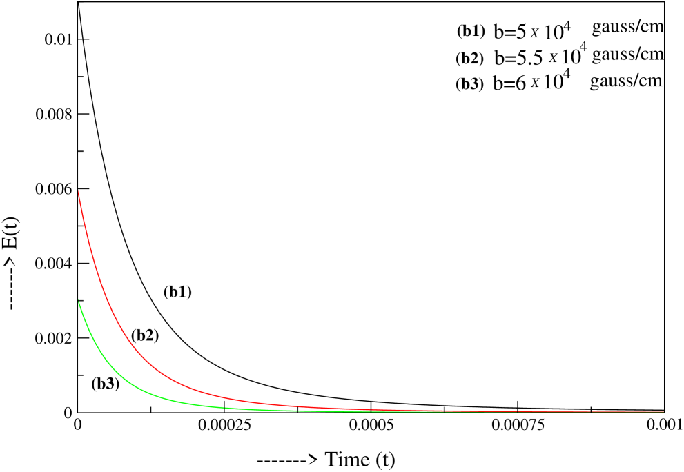
Figure 2: The variation of $E(t)$ with time (in sec) is shown for three different values of $b$, i.e., $b=5\times 10^{4}gauss/cm$, $b=5.5\times 10^{4}gauss/cm$ and $b=6\times 10^{4}gauss/cm$ with $\tau=5\times 10^{-4}sec$ and $\sigma_{0}=10^{-5}cm$ while $E_{s}=0$ and $|I|=0$. [CASE (i)]

As we have defined above, $|I|=0$ implies the formally ideal situation, and $E_{s}=0$ the operationally ideal situation. Within the context of the nonideal Stern-Gerlach experiment, it is then possible to identify the following distinct situations which highlight the possible connections between configuration space orthogonality and position space distinguishability.

(i) If the situation is operationally ideal ($E_{s}=0$), then it must be formally ideal $(|I|=0)$. Or in other words, the observation of position space distinguishability implies that the two wave functions are orthogonal in configuration space.

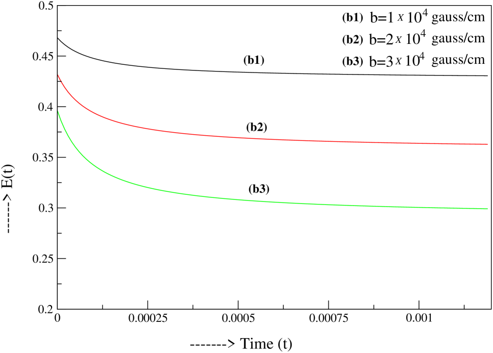
Figure 3: The variation of $E(t)$ with time (in sec) is shown for the values $b=1\times 10^{3}gauss/cm$, $b=2\times 10^{3}gauss/cm$ and $b=3\times 10^{3}gauss/cm$, respectively, with $\tau=10^{-4}sec$ and $\sigma_{0}=10^{-4}cm$ while $E_{s}\neq 0$ and $|I|\neq 0$. [CASE (ii)]

(ii) If the situation is formally nonideal ($|I|\neq 0$), then it must be operationally nonideal ($E_{s}\neq 0$). This means that any non-orthogonality in the configuration space translates into the overlap of the spatial wave functions, and this represents the usual nonideal situation which has been studied by earlier authorsalstrom ; cruz with the aim of reducing the magnitude of nonidealness.

(iii) If the situation is formally ideal ($|I|=0$), it still may be operationally nonideal ($E_{s}\neq 0$). This is the most interesting outcome of our present study since this hitherto unexplored nonideal situation implies that formal idealness or configuration space orthogonality does not always guarantee operational idealness in terms of position space distinguishability.

IV Quantitative estimates of operational versus formal nonidealness

We will now show explicitly how the different situations (i), (ii) and (iii) arise due to the choices of the parameters in the SG experiment. In order to illustrate these features, we present some numerical estimates for the probabilities $P_{\uparrow}^{ni}$ and $P_{\downarrow}^{ni}$, and $P_{+}^{ni}$ and $P_{-}^{ni}$ given in Eqs.(13) and (14) respectively. The estimation of these probabilities is contingent on the values of $\alpha$, $\beta$ and $E_{s}$. We first show three representative figures (Fig.2, Fig.3 and Fig.4) corresponding to the situations (i), (ii) and (iii) respectively, which indicate how the parameter $E(t)$ varies with time and saturates to $E_{s}$ (which is not always zero). The curves in the figures are plotted by taking various choices of the relevant parameters, such as the degree of inhomogeneity of the magnetic field $b$, and the interaction time $\tau$ while the initial width of the Gaussian wave packet $\sigma_{0}$ and the mass $m$ of the neutron are fixed.

Figure 4: The variation of $E(t)$ with time (in sec) is shown for the values $b=2\times 10^{4}gauss/cm$, $b=3\times 10^{4}gauss/cm$ and $b=4\times 10^{4}gauss/cm$, respectively, with $\tau=10^{-4}sec$ and $\sigma_{0}=10^{-5}cm$ while $E_{s}\neq 0$ although $|I|=0$. [CASE (iii)]

Corresponding to the above three cases, we further plot the snapshots of the overlap between $|\psi_{+}(z,t)|^{2}$ and $|\psi_{-}(z,t)|^{2}$ (Figs.5, 6 and 7) for three different sets (Set-I, Set-II and Set-III) of the relevant parameters $\tau$, $b$, and $\sigma_{0}$ at two different times $t=10^{-5}sec$ and $t=0.1sec$. For Set-I, $b=6\times 10^{4}gauss/cm$, $\tau=5\times 10^{-4}sec$ and $\sigma_{0}=10^{-5}cm$. For Set-II, $b=2\times 10^{3}gauss/cm$, $\tau=10^{-4}sec$ and $\sigma_{0}=10^{-4}cm$ . For Set-III, $b=4\times 10^{4}gauss/cm$, $\tau=10^{-4}sec$ and $\sigma_{0}=10^{-5}cm$. These Set-I, Set-II and Set-III correspond to the three situations (i), (ii) and (iii) respectively as discussed earlier. One can see from Fig.7 that there exists a finite and appreciable overlap between the $|\psi_{+}({\bf x},t)|^{2}$ and $|\psi_{-}({\bf x},t)|^{2}$ at $t=10^{-5}sec$ which does not always vanish at $t=0.1sec$ (which is much larger than the saturation time $t_{s}$), although the inner product $|I|$ is zero.

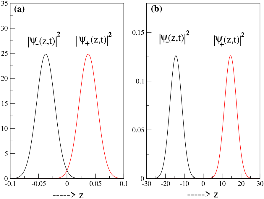
Figure 5: The overlap between $|\psi_{+}(z,t)|^{2}$ and $|\psi_{-}(z,t)|^{2}$ is plotted for $b=6\times 10^{4}gauss/cm$, $\tau=5\times 10^{-4}sec$ and $\sigma_{0}=10^{-5}cm$ at two different times (a) $t=10^{-5}sec$, and (b) $t=0.1sec$ while $|I|=0$ and $E_{s}=0$. [CASE (i)]

We now use the parameters of Set-III to calculate the probabilities for finding spin up $P_{\uparrow}^{ni}$ and spin down $P_{\downarrow}^{ni}$ particles from Eq.(13) in the formally ideal but operationally nonideal situation [CASE (iii)] and the corresponding probabilities $P_{+}^{ni}$ and $P_{-}^{ni}$ in the upper and lower planes, respectively from Eq.(14). We choose four different values for $\alpha$ and $\beta$ satisfying $|\alpha|^{2}+|\beta|^{2}=1$. The saturation value of $E_{t}$ is obtained to be $E_{s}=0.2478$. The results are presented in Table 1.

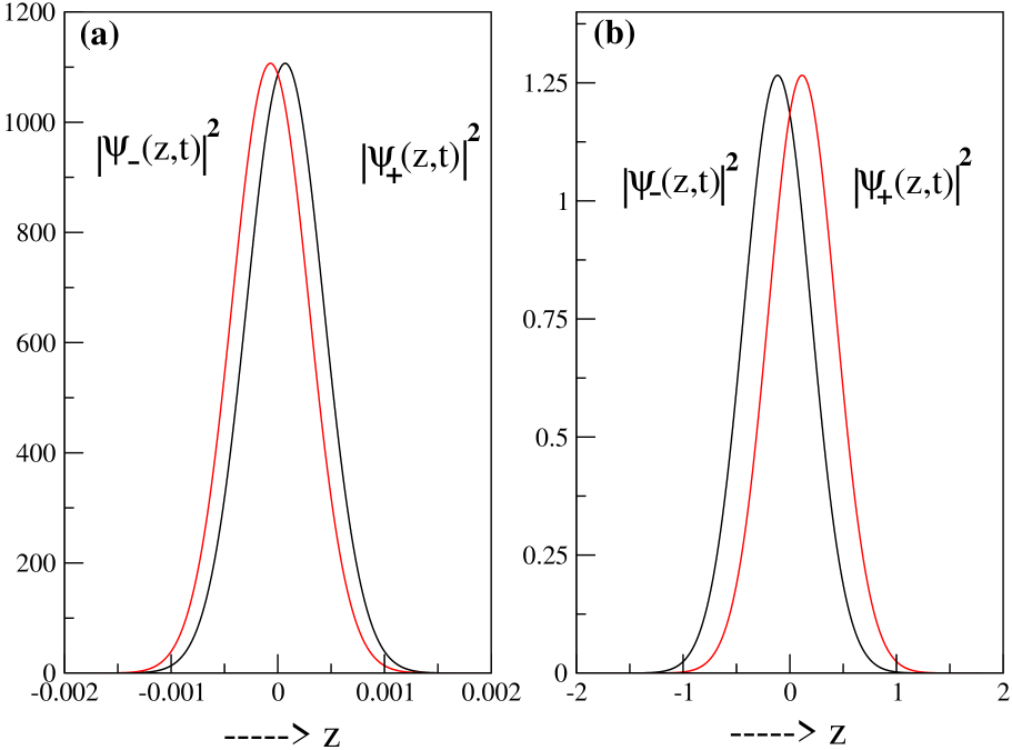
Figure 6: The overlap between $|\psi_{+}(z,t)|^{2}$ and $|\psi_{-}(z,t)|^{2}$ is plotted for $b=2\times 10^{3}gauss/cm$, $\tau=10^{-4}sec$ and $\sigma_{0}=10^{-4}cm$ at two different times (a) $t=10^{-5}sec$, and (b) $t=0.1sec$ while $|I|\neq 0$ and $E_{s}\neq 0$. [CASE (ii)]

It is seen from the Table 1 that when $\alpha=\beta=1/\sqrt{2}$ the probability of finding particles with both $\left|\uparrow\right\rangle$ and $\left|\downarrow\right\rangle$ spins in the upper plane is $P_{+}^{ni}=0.5000$ where probability of finding $\left|\uparrow\right\rangle$ (and $\left|\downarrow\right\rangle$) in the upper plane is $P_{\uparrow}^{ni}=0.3761$ (and $=0.1239$). Note that, in the usual ideal situation (i) the probability of finding particles with $\left|\uparrow\right\rangle$ in the upper plane is $P_{+}^{i}=P_{\uparrow}^{i}=0.5000$. To test the result experimentally, a subsequent SG setup which is ideal in the sense of our situation (i), i.e., $|I|=0$ and $E_{s}=0$, needs to be suitably placed. The position of the second SG setup as well as the final screen position must be beyond the corresponding saturation position $Y_{s}=v_{y}t_{s}$. The vaule of $t_{s}$ and subsequently $E_{s}$ is different for different parameter choices. For the parameters chosen in the Table 1, $t_{s}=0.0012sec$ and hence the possible position of the second SG setup $Y_{s}$ is beyond $12cm$ if one takes $v_{y}=10^{4}cm/sec$.

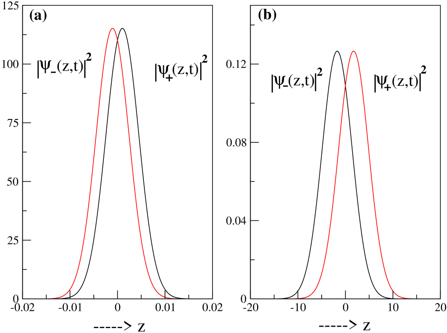
Figure 7: The overlap between the $|\psi_{+}(z,t)|^{2}$ and $|\psi_{-}(z,t)|^{2}$ is plotted for $b=4\times 10^{4}gauss/cm$, $\tau=10^{-4}sec$ and $\sigma_{0}=10^{-5}cm$ at two different times (a) $t=10^{-5}sec$, and (b) $t=0.1sec$ while $|I|=0$ but $E_{s}\neq 0$. [CASE (iii)]

$\alpha$	$\beta$	$P_{\uparrow}^{i}=P_{+}^{i}$	$P_{\downarrow}^{i}=P_{-}^{i}$	$P_{\uparrow}^{ni}$	$P_{\downarrow}^{ni}$	$P_{+}^{ni}$	$P_{-}^{ni}$
$1/\sqrt{2}$	$1/\sqrt{2}$	0.5000	0.5000	0.3761	0.3761	0.5000	0.5000
0.8000	0.6000	0.6400	0.3600	0.4814	0.2708	0.5706	0.4294
$\sqrt{3}/2$	$1/2$	0.7500	0.2500	0.5642	0.1881	0.6261	0.3739
0.9487	0.3162	0.9000	0.1000	0.6770	0.0752	0.7018	0.2982

TABLE.1: The quantities $P^{i}_{\uparrow}$ and $P^{i}_{\downarrow}$ denote the observable probabilities for finding respectively, the spin up and spin down particles corresponding to $\left|\uparrow\right\rangle_{z}$ and $\left|\downarrow\right\rangle_{z}$ of the ideal SG measurement and $P^{ni}_{\uparrow}$ and $P^{ni}_{\downarrow}$ are the same for the nonideal case. The quantities $P^{i}_{+}$ and $P^{i}_{-}$ denote the observable probabilities of finding particles in the upper plane and in the lower plane of the ideal SG measurement and $P^{ni}_{+}$ and $P^{ni}_{-}$ are the same for the nonideal case. Note that $P^{i}_{\uparrow}=P^{i}_{+}$ and $P^{i}_{\downarrow}=P^{i}_{-}$. In this Table the results are presented for four different choices of $\alpha$ and $\beta$ satisfying $|\alpha|^{2}+|\beta|^{2}=1$ with $E_{s}=0.2478$ for the relevant parameters $b=4\times 10^{4}gauss/cm$, $\tau=10^{-4}sec$ and $\sigma_{0}=10^{-5}cm$ while $|I|=0$. [CASE (iii)]

V Summary and Conclusions

In this paper we have probed the usually implied assumption in the theory of quantum measurement that the configuration space orthogonality between the wave functions necessarily entails their unambiguous position space separability. While the latter is a key operational concept used to infer the outcomes of the SG experiment, our results show that the validity of the above assumption can be ensured only for specific choices of relevant parameters. It is demonstrated that there is indeed a range of possible choices that can lead to non-ideal situations where the above assumption is clearly falsified. Thus even a formally ideal measurement situation in quantum mechanics where the states are orthogonal in configuration space does not necessarily imply an unambiguous separation of states in the position space which characterises an operationally ideal measurement.

The non-idealness of the above kind where the overlap between the wave packets in the position space persists even at large distance in spite of the orthogonality of the corresponding configuration space states has remained hitherto unexplored. It is thus important to evaluate theoretically in a formally ideal $|I|=0$ but operationally non-ideal$(E_{s}\neq 0)$ situation as to what will be the possible outcomes of the SG experiment when it is used in its various applications bohm ; wigner ; eng ; robert ; oliv ; reini ; duerr ; knight mentioned in the beginning. For this purpose we’ve defined an error integral $E(t)$ which is used to quantify the results of the nonideal situations where the probabilities for finding spin up particles in the lower plane and for finding spin down particles in the upper plane are both non-vanishing. We find that the saturation value of the error integral $E_{s}$ can be non-zero for a wide range of the relevant parameters such as the inhomogeneity of the magnetic field $b$ and the SG interaction time $\tau$. Thus, in non-ideal situations, we can predict the observable outcomes, i.e., the probabilities $P_{+}^{ni}$ and $P_{-}^{ni}$ corresponding to both spin up and spin down particles in the upper and lower planes respectively. These predictions can be experimentally verified by placing a subsequent completly ideal (both formally and operationally) SG device at a suitable distance in accordance with the values of the relevant parameters.

The utility of such a scheme for quantifying the nonidealness in any given SG setup lies in enabling the estimation of error involved in inferring the measured spin state (i.e., the error in the state reconstruction process) from the actual measurement results. That this situation may arise even in the formally ideal case with orthogonal states adds further practical relevance to the estimation of the observable outcomes.

To summarize, we have demonstrated that in a nonideal SG setup, conditions can be achieved for suitable choices of relevant parameters so that a significant spatial overlap between the emerging wave packets persists even when the inner product between the emergent wave functions is zero. Potential uses of variants of this type of nonideal SG setup as a resource need to be explored in detail, particularly in regard to foundational issues such as the contentious question as to when a quantum measurement is completedhome . Furthermore, the analysis of operational non-idealness is likely to have quantitative implications in the SG interferometry. For example, one can attempt a non-ideal variant of an interesting example of quantum-state reconstruction hradil involving analysis of a synthesis of noncommuting observables of spin-1/2 particles using SG device with varying orientations. As indicated by Hradil et al. hradil , the formalism developed for the analysis of such examples can be applied to the study of various problems like the estimation of the quantum state inside split beam neutron interferometers. Finally, we note that since the effect of enviournment induced decoherence on the position space overlap of the wave packets has been studied in an ideal SG setupvenu , it should be interesting to investigate such effects in the types of non-ideal SG setup discussed in this paper.

Acknowledgements

We are grateful to John Corbett for helpful discussions. DH acknowledges support from the Jawaharlal Nehru Fund, India. AKP acknowledges support from the Council of Scientific and Industrial Research, India.

References

- (1) J. von Neumann, Mathematical Foundations of Quantum Mechanics,(Princeton University Press, Princeton, 1966).
- (2) D. Home, Conceptual Foundations of Quantum Physics,(Plenum Press, New York, 1997), Ch.2.
- (3) A. J. Leggett, J. Phys.: Condens. Matter 14, R415 (2002).
- (4) W. Gerlach and O. Stern, Z. Phys. 9, 349 (1922).
- (5) D. Bohm,Quantum theory, (Prentice-Hall, Englewood Cliffs, NJ, 1952).
- (6) E. P. Wigner, Am. J. Phys. 31, 6 (1963).
- (7) B. G. Englert, J. Schwinger and M. O.Scully, Found.phys. 18, 1045 (1988); M. O. Scully, J. Schwinger and B. G. Englert,Z. Phys. D 10, 135 (1988); M. O. Scully, B. G. Englert and J. Schwinger, Phys. Rev. A 40, 1775 (1989).
- (8) C. Minitura, J. Robert, O. Gorceix, V. Lorent, S. Le Boiteux, J. Reinhardt, J. Baudon , Phys. Rev. Lett. 69, 261 (1992); J. Robert, O.Gorceix, J. Lawson-Daku, S. Nic Chomaric, C. Minitura, J. Baudon, F. Peralls, M. Eminyar and K. Rubin, in: D. M. Greenberger and A. Zeilinger (Eds.), Fundamental Problems in Quantum Theory, Part III, Ann (NY) Acad. Sc., 755, 173 (1995).
- (9) T. de Oliveria and A. Calderia, Phys. Rev. A73, 042502 (2006).
- (10) G. Reinisch, Phys. Lett. A 259, 427 (1999).
- (11) S. Duerr, T. Nonn and G. Rempe, Nature 395, 33 (1998).
- (12) P. Knight, Nature 395, 12 (1998).
- (13) P. Alstrom, P. Hjorth and R. Muttuck, Am. J. Phys. 50, 697 (1982); S. Singh and N. K. Sharma, Am. J. Phys. 52, 274 (1983).
- (14) S. Cruz-Barrios and J. Gomez-Camacho, Phys. Rev. A 63, 012101 (2000); Phys. Rev. A 71, 052106 (2005).
- (15) M. O. Scully, W.E. Lamb, Jr. and A. Barut, Found. Phys. 17, 575 (1987); P. Busch and F. E. Schroeck, Jr., Found. Phys. 19, 807 (1989); D. E. Platt, Am. J. Phys. 60, 306 (1992); G. B. Roston, M. Casas, A. Plastino and A. R. Plastino, J. Phys. A 26, 657 (2005).
- (16) I. D. Ivanovic, Phys. Lett. A 123, 257 (1987); D. Dieks, Phys. Lett. A 126, 303 (1988); A. Peres, Phys Lett. A 128, 19 (1988); A. Chefles, Contemp. Phys. 41, 401 (2000).
- (17) Z. Hradil, J. Summhammer, G. Badurek and H. Rauch, Phys. Rev A 62, 014101 (2000).
- (18) A. Venugopalan, Phys. Rev. A 56, 4307 (1997); Phys. Rev. A 61, 012102 (2000).