Nonlocality improves Deutsch algorithm

Abstract

Recently, [arXiv:0810.3134] is accepted and published. We show that the Bell inequalities lead to a new type of linear-optical Deutsch algorithms. We have considered a use of entangled photon pairs to determine simultaneously and probabilistically two unknown functions. The usual Deutsch algorithm determines one unknown function and exhibits a two to one speed up in a certain computation on a quantum computer rather than on a classical computer. We found that the violation of Bell locality in the Hilbert space formalism of quantum theory predicts that the proposed probabilistic Deutsch algorithm for computing two unknown functions exhibits at least a $2\sqrt{2}(\simeq 2.83)$ to one speed up.

I Introduction

Recently, NagataNakamura is accepted and published. Quantum information processing and quantum computing have attracted much interest in science community because of their novel usage of quantum mechanics in technological applications. Many ideas of quantum processors and computers were experimented in many architectures of physical systems, including ion traps, neutral atoms, nuclear spins in magnetic resonance, semiconductor quantum dots, and super-conducting resonators IONTRAPQC ; ATOMQC ; NMRQC ; QuantumDotQC ; SCQC . Still the progress has been limited to a few qubit operations and the performance is far from being practical. The ability of quantum computers in outperforming their classical counterparts has not been demonstrated.

In many physical systems, the preparation and change of quantum states, or how to prepare entanglements and how to maintain coherence, is a more difficult task than how to wire logics quantum-mechanically. However, in quantum computing with linear optical systems, it is relatively easy to deal with entanglement and decoherence. For this reason, linear optical quantum computings or the linear interactions of photons with matters are often adopted for the implementation of $N$-qubit quantum algorithms AhnScience2000 ; BhattacharyaPRL2002 . Especially entanglement is an important aspect that a quantum mechanical device can have and the quantum information carried by an entangled state like Einstein, Podolsky, and Rosen (EPR) state overcomes some of the limitations of classical information used in communication and cryptography NC ; Galindo ; CRYPTOGRAPHY ; BRUKNER_PRL . Recently, there have been several attempts to use single-photon two-qubit states for quantum computing. Oliveira et al. implemented the Deutsch algorithm with polarization and transverse spatial modes of the electromagnetic field as qubits Oliveira . Single-photon Bell states were prepared and measured by Kim Kim2003 . Also the decoherence-free implementation of Deutsch algorithm using such single-photon two logical qubits Mohseni2003 . Although such a single-photon two-qubit implementation is not scalable, the quantum gates necessary for information processing can be implemented deterministically using only linear optical elements.

Often a demonstration of quantum algorithm, which is performed with possibly mixed quantum states, is presented without a proper mathematical theory for the analysis of experimental data, or with a rather complicated quantum tomographical state analysis. However, if the output state of an experiment under study should be an entangled state, we can choose to use Bell inequalities BELL . It is a sufficient condition to demonstrate a negation of Bell locality and the detection of entanglement. We can consider the following question. Is there a relationship between the negation of Bell locality and the performance of such quantum algorithm that can be implemented by a single photon? Interestingly the answer is yes.

In this paper we have devised an experimental scheme to obtain simultaneous and nonlocal answers from Deutsch problem with two unknown functions. Especially we elaborate the use of entanglement in processing this quantum algorithm. The advantage of using an EPR pair of photons (two-photon two-qubit states) in quantum computing algorithm is analyzed with Bell inequalities in quantum theory. We show that a set of answers of the given Deutsch problem, with two unknown functions, statistically shows a violation of Bell locality in the Hilbert space formalism of quantum theory. It turns out that the negation of Bell locality exhibits a $2\sqrt{2}$ to one speed up at least. We, thus, observe a highly nonlocal effect and it leads the entangled answers in a network of pair quantum computers to provide enhanced information compared with its classical counterpart. An important note here is that there must be probabilistic errors in answers which appear due to the imperfection of the photon detection and defects in optical devices. Thus it is necessary to take into account many measurements and what we can do is only to analyze probabilistically in real experimental situation. By applying the maximum likelihood principle, the answer to the Deutsch problem is estimated probabilistically.

In the following sections, we introduce a method of linear optical quantum computing of Deutsch problem. In the section II, the method that utilizes two-photon two-qubit entanglement is discussed. This method allows statistical analysis of the average value of Bell operator. In order to overcome the imperfection of the photon detection and possible defects in optical devices, the fidelity NAGATA1 of the method is analyzed. During the analysis of Bell operator or the fidelity to EPR state in Sec. III, the separable states are distinguished from the entangled states. It is well known that the fidelity which is larger than $1/\sqrt{2}$ to EPR state is a sufficient condition for a negation of Bell locality in the Hilbert space formalism of quantum theory. We can say that our Deutsch scheme succeeds with the probability of the value of the lower bound of fidelity at least under the condition where the fidelity is larger than $1/\sqrt{2}$. A short summary and conclusion follows in Sec. IV.

II Deutsch algorithm with two unknown functions

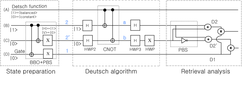
Figure 1: The schematic of Deutsch algorithm with a two-photon state. The classical channel (A) represents the type of the chosen Deutsch function. The two quantum channels (B) and (C), in a superposition single-photon state, are initially prepared in a horizontally polarized state, $|1\rangle$, and a vertically polarized state, $|0\rangle$, respectively. The channel (D) is for the extra photon for a time correlation detection.

The Deutsch algorithm determines whether a given function, $f(x)$, on a binary number, $x$, is either balanced or constant, where the function is constant if the function outputs for $x=0$ and $1$ are the same and balanced if not. The unknown function is defined by

$$U_{f}|x\rangle_{y}\equiv|x\rangle_{y\oplus f(x)}.$$ (1)

In a classical computer the answer is obtained by calculating $f(0)$ and $f(1)$, while in a quantum computer only a single calculation with a superposition state of $0$ and $1$ is necessary. Hence, if $f(H)=f(V)$ then the output label should not depend on $H$ and $V$, whereas if $f(H)\neq f(V)$ then the output label should depend on $H$ and $V$.

As shown in Fig. 1, Deutsch algorithm can be implemented using a two-photon state. The quantum channels (B) and (C) represent the horizontally polarized photon, in a superposition state coherently traveling along two paths 2 and 2’, from an EPR photon pair. The qubits in these channels are to be simultaneously altered by the control bit in channel (A) that denotes $|1\rangle$ for a balanced function or $|0\rangle$ for a constant function. Then the final photon state, which is collapsed and detected either at the detector D2 or D2’, reveals the type of the Deutsch function: whether the unknown function was balanced or constant. The other photon, in the vertical polarization, is used as a gate function for the coincidence measurement. This is reminiscent of Oliveira’s scheme in Oliveira , except that we discuss quantum-mechanical advantage of wiring two of those Deutsch algorithms which are simultaneously processed by an entangled two-photon state.

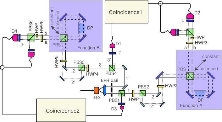
Figure 2: The Deutsch algorithm with a two-photon entangled state

We describe the experimental scheme shown in Fig. 2. The unknown functions $A$ and $B$ in the gray boxes represent the CNOT gate in Fig 1. The half-wave-plates labeled from HWP1 to HWP5, oriented at $\theta=22.5^{\circ}$, are the Hadamard gates, which change a horizontal (vertical) polarization state into a 45^∘ (45^∘) polarization state. The half-wave-plates labeled as HWP in Fig. 2 are oriented at $\theta=45^{\circ}$ and swap the horizontal and vertical polarizations, like the $X$ gates in Fig 1. In our implementations, we assign the truth values 0 and 1 as $|H\rangle\leftrightarrow|1\rangle,~{}|V\rangle\leftrightarrow|0\rangle$. The initial photon is in the coherent superposition state of $(|1\rangle_{2}+|0\rangle_{2^{\prime}})/\sqrt{2}$. Then, the state evolution after the logic gates $H$ and $V$ depending on the choice of the unknown Deutsch function, $X$ for the balanced function or $I$ for the constant function, becomes

$$H\left[\begin{tabular}[]{c}$X$\\ $I$\end{tabular}\right]H|1\rangle+\alpha XH\left[\begin{tabular}[]{c}$X$\\ $I$\end{tabular}\right]H|0\rangle=\left[\begin{tabular}[]{c}$1-\alpha$\\ $1+\alpha$\end{tabular}\right]|1\rangle,$$ (8)

where the detector D2 clicks if $\alpha=1$ and D2’ clicks if $\alpha=-1$.

This scheme is the generalization of the usual Deutsch algorithm in such a way that we can determine the lower bound of the success probability of the algorithm and we can see a violation of Bell locality in the Hilbert space formalism of quantum theory. In this section, we consider an ideal case, i.e., there is not any experimental noise to simplify the discussion. However, in real experimental situations, we have to take error answers into account due to experimental imperfections. Thus, many runs of experiments are evidently necessary. Hence, we shall discuss a method using Bell operators to analyze experimental data. The method of such analysis will be presented in Sec. III.

We use Pauli observables for the representation of photon polarization states as

$$\sigma_{z} = |H\rangle\langle H|-|V\rangle\langle V|,$$

$$\sigma_{x} = |H\rangle\langle V|+|V\rangle\langle H|.$$ (9)

The initial state of photons is an EPR bi-photon state as

$$\frac{1}{\sqrt{2}}(|V\rangle_{1}|H\rangle_{1^{\prime}}-|H\rangle_{1}|V\rangle_{1^{\prime}}).$$ (10)

Now we follow the time evolution of each of photons.

II.1 Deutsch algorithm with a function A

Assume that the case where the state $|H\rangle_{1}|V\rangle_{1^{\prime}}$ is contributed to our Deutsch algorithm. In this case, the unknown function (A) is determined as constant or balanced. After HWP1, the each state of photons becomes

$$|H\rangle_{1}\rightarrow\frac{|H\rangle_{1}+|V\rangle_{1}}{\sqrt{2}},\quad|V\rangle_{1^{\prime}}\rightarrow|V\rangle_{D1}.$$ (11)

Hence the state $|H\rangle_{1}|V\rangle_{1^{\prime}}$ becomes

$$\frac{1}{\sqrt{2}}(|H\rangle_{1}+|V\rangle_{1})|V\rangle_{D1}.$$ (12)

A vertically polarized photon is detected by the $D1$ detector. That is,

$$\sigma^{D1}_{z}=-1.$$ (13)

We see that the state of the photons $\frac{1}{\sqrt{2}}(|H\rangle_{1}+|V\rangle_{1})|V\rangle_{D1}$ is projected into the following $(|H\rangle_{1}+|V\rangle_{1})/\sqrt{2}$. In order to simplify the discussion, in what follows, we consider this state. The polarizing beam splitter (PBS2) changes each of states as $|H\rangle_{1}\rightarrow|H\rangle_{2},~{}|V\rangle_{1}\rightarrow|V\rangle_{2^{\prime}}$. Hence we have

$$\frac{1}{\sqrt{2}}(|H\rangle_{2}+|V\rangle_{2^{\prime}}).$$ (14)

After the half-wave plate (HWP2) each of the states becomes as

$$|H\rangle_{2}\rightarrow\frac{|H\rangle_{2}+|V\rangle_{2}}{\sqrt{2}},\quad|V\rangle_{2^{\prime}}\rightarrow\frac{|H\rangle_{2^{\prime}}-|V\rangle_{2^{\prime}}}{\sqrt{2}}.$$ (15)

From state (14), after HWP2, we have

$$\frac{1}{\sqrt{2}}\bigg{(}(\frac{|H\rangle_{2}+|V\rangle_{2}}{\sqrt{2}})+(\frac{|H\rangle_{2^{\prime}}-|V\rangle_{2^{\prime}}}{\sqrt{2}})\bigg{)}.$$ (16)

A dove prism (DP) is the most important part in implementing the given functions. The output polarization state of the dove prism rotates at twice the angular rate of the rotation of the prism itself. So, if a dove prism inclines at $45^{\circ}$ about a vertical line, the image rotates at $90^{\circ}$. Now we consider how a CNOT gate (cf. CNOT ) is implemented with the space and polarization degrees of freedom of a photon. As shown in Fig. 3, a horizontally polarized photon is transmitted through the polarization beam splitter. But a vertically polarized photon is reflected at the polarization beam splitter. They propagate along different ways. The angle between a vertical line and the axis of the dove prism is $45^{\circ}$ in the case of a horizontally polarized photon, but $-45^{\circ}$ in the other case. So this configuration implements such changes of photon paths: $2\rightarrow a$, $2^{\prime}\rightarrow b$ when the polarization is horizontal. $2\rightarrow b$, $2^{\prime}\rightarrow a$ when the polarization is vertical. Here $a$ and $b$ are the labels for the paths toward detectors. Output photons labeled by $a$ and $b$ are detected by $D2$.

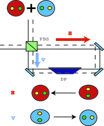
Figure 3: An example of polarization-CNOT gates

II.1.1 Balanced function case

In the balanced function case, the changes of the polarization states of the photons due to the dove prism are:

$$|H\rangle_{2}\rightarrow|H\rangle_{a},~{}|H\rangle_{2^{\prime}}\rightarrow|H\rangle_{b},$$

$$|V\rangle_{2}\rightarrow|V\rangle_{b},~{}|V\rangle_{2^{\prime}}\rightarrow|V\rangle_{a}.$$ (17)

Thus, after the dove prism, the state (16) becomes

$$\frac{1}{\sqrt{2}}\bigg{(}(\frac{|H\rangle_{a}+|V\rangle_{b}}{\sqrt{2}})+(\frac{|H\rangle_{b}-|V\rangle_{a}}{\sqrt{2}})\bigg{)}.$$ (18)

After HWP3, we have $(|V\rangle_{a}+|H\rangle_{b})/\sqrt{2}$. After HWP($\theta=45^{\circ}$), we get $(|V\rangle_{a}-|V\rangle_{b})/\sqrt{2}$. Hence, we detect only vertically polarized photons in $D2$. This implies

$$(\sigma^{a}_{z}=\sigma^{b}_{z}=)\sigma^{D2}_{z}=-1.$$ (19)

Hence from Eqs. (13) and (19) the value of observable $\sigma^{D1}_{z}\sigma^{D2}_{z}$ should be $+1$. This is one of the success result of a single run of the experiment, i.e.,

$$\sigma^{D1}_{z}\sigma^{D2}_{z}=+1.$$ (20)

II.1.2 Constant function case

After the dove prism, polarized photon states changes as follows

$$|H\rangle_{2}\rightarrow|H\rangle_{a},~{}|H\rangle_{2^{\prime}}\rightarrow|H\rangle_{b},$$

$$|V\rangle_{2}\rightarrow|V\rangle_{a},~{}|V\rangle_{2^{\prime}}\rightarrow|V\rangle_{b}.$$ (21)

Thus, after the dove prism, the state (16) becomes

$$\frac{1}{\sqrt{2}}\bigg{(}(\frac{|H\rangle_{a}+|V\rangle_{a}}{\sqrt{2}})+(\frac{|H\rangle_{b}-|V\rangle_{b}}{\sqrt{2}})\bigg{)}.$$ (22)

After HWP3 we have $(|H\rangle_{a}+|V\rangle_{b})/\sqrt{2}.$ After HWP($\theta=45^{\circ}$), we have $(|H\rangle_{a}+|H\rangle_{b})/\sqrt{2}.$ Hence, we detect only horizontally polarized photons in $D2$. This implies

$$(\sigma^{a}_{z}=\sigma^{b}_{z}=)\sigma^{D2}_{z}=+1.$$ (23)

Hence from Eqs. (13) and (23) the value of observable $\sigma^{D1}_{z}\sigma^{D2}_{z}$ should be $-1$. This is one of the success result of a single run of the experiment, i.e.,

$$\sigma^{D1}_{z}\sigma^{D2}_{z}=-1.$$ (24)

Thereby, we can determine whether a given function (A) is constant or balanced with utilizing the state $|H\rangle_{1}|V\rangle_{1^{\prime}}$.

II.2 Deutsch algorithm with a function B

Similarly we can assume that the case where the state $|V\rangle_{1}|H\rangle_{1^{\prime}}$ is contributed to our Deutsch algorithm. In this case, the unknown function (B) is determined in constant one or balanced one. At the detector $D3$ the photon state becomes $(|H\rangle_{1}+|V\rangle_{1})|V\rangle_{D3}/\sqrt{2}.$ So a vertically polarized photon is detected by the $D3$ detector. That is,

$$\sigma^{D3}_{z}=-1.$$ (25)

Therefore in the balanced function case, the changes of the polarization states of the photons due to the dove prisms, HWP6 and the last HWP($\theta=45^{\circ}$) are: $(|V\rangle_{a}-|V\rangle_{b})/\sqrt{2}.$ Hence, we detect only vertically polarized photons in $D4$. This implies

$$(\sigma^{a}_{z}=\sigma^{b}_{z}=)\sigma^{D4}_{z}=-1.$$ (26)

Hence from Eqs. (25) and (26) the value of observable $\sigma^{D3}_{z}\sigma^{D4}_{z}$ should be $+1$. This is one of the result of a single run of the experiment, i.e.,

$$\sigma^{D3}_{z}\sigma^{D4}_{z}=+1.$$ (27)

In the constant function case, similarly we get after the dove prisms, HWP6 and the last HWP($\theta=45^{\circ}$) $(|H\rangle_{a}+|H\rangle_{b})/\sqrt{2}.$ And, we detect horizontally polarized photons in $D4$. This implies

$$(\sigma^{a}_{z}=\sigma^{b}_{z}=)\sigma^{D4}_{z}=+1.$$ (28)

Hence from Eqs. (25) and (28) the value of observable $\sigma^{D3}_{z}\sigma^{D4}_{z}$ should be $-1$. This is one of the success result of a single run of the experiment, i.e.,

$$\sigma^{D3}_{z}\sigma^{D4}_{z}=-1.$$ (29)

Thereby, we can determine whether a given function (B) is constant or balanced with utilizing the state $|V\rangle_{1}|H\rangle_{1^{\prime}}$.

Thus, we can determine whether either a given function (A) or (B) is constant or balanced with utilizing EPR entanglement. Clearly, many EPR experiments evaluate two functions simultaneously, i.e, Deutsch algorithm exhibiting a four to one speed up. In the next section, we assume the existence of experimental imperfections and we present the method to determine the lower bound of the success probability of our scheme presented by Fig. 2. Especially, a violation of Bell locality in the Hilbert space formalism of quantum theory ensure the success probability is larger than $1/\sqrt{2}$.

III Bell operator analysis

In the previous section, we have assumed that the initial state is a two-photon entangled state $|\Psi\rangle=(|V\rangle_{z}|H\rangle_{z}-|H\rangle_{z}|V\rangle_{z})/\sqrt{2}$. We now insert a polarizer oriented at $45^{\circ}$ and a HWP ($\lambda/2$ plate) in front of each detector. See Fig. 4. This allows the measurement of polarized photon states described in polarized basis $x$. That is, one can measure an observable $\sigma_{x}$ in this way. Due to the feature of the initial state, the same situation occurs in the ideal case. The situation is as follows. One can see

$$|H\rangle_{x}=\frac{|H\rangle_{z}+|V\rangle_{z}}{\sqrt{2}},$$

$$|V\rangle_{x}=\frac{|H\rangle_{z}-|V\rangle_{z}}{\sqrt{2}}.$$ (30)

Let us rewrite the initial state $|\Psi\rangle$ using $x$ polarization basis. We have $|\Psi\rangle=(|V\rangle_{x}|H\rangle_{x}-|H\rangle_{x}|V\rangle_{x})/\sqrt{2}$. This implies that the scheme mentioned in the preceding section works in the same way. However, we have to take the imperfection of the photon detection and defects in optical device into account.

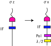
Figure 4: A setup of measurement of polarization in $z$ basis and in $x$ basis

Here we introduce Bell operators:

$$B_{A}=\frac{1}{\sqrt{2}}(\sigma^{D1}_{x}\sigma^{D2}_{x}+\sigma^{D1}_{z}\sigma^{D2}_{z})$$

$$B_{B}=\frac{1}{\sqrt{2}}(\sigma^{D3}_{x}\sigma^{D4}_{x}+\sigma^{D3}_{z}\sigma^{D4}_{z}).$$ (31)

First of all, we check if both of the following Bell inequalities BELL are violated:

$$|\langle B_{A}\rangle_{\rm avg}|\leq 1,~{}|\langle B_{B}\rangle_{\rm avg}|\leq 1.$$ (32)

When both of the Bell inequalities are violated, we can ensure that the success probability of our Deutsch algorithm is larger than $1/\sqrt{2}$ in the experiment as shown below.

We note here that if experimental error exits one could misjudge the unknown function. For instance, it is possible that actually observed data says that the unknown function is constant even though the unknown function is in fact balanced. Such a wrong case occurs when experimental error is larger than a half. Nevertheless, our analysis rules out such a wrong case since a violation of two Bell inequalities ensures the success probability of our scheme is larger than $1/\sqrt{2}$.

In Table 1, we summarize the relationship between a violation of Bell inequalities and the two types of functions ($A$) and ($B$).

	$A$	$B$
Balanced	$\langle B_{A}\rangle_{\rm avg}>1$	$\langle B_{B}\rangle_{\rm avg}>1$
Constant	$\langle B_{A}\rangle_{\rm avg}<-1$	$\langle B_{B}\rangle_{\rm avg}<-1$

Table 1: The rationship between the the violation of Bell inequalities and the two kinds of functions ($A$) and ($B$).

The situation is as follows. First, we consider the case in which the unknown function (A) is balanced. The fidelity to $(|H\rangle_{D1}|H\rangle_{D2}+|V\rangle_{D1}|V\rangle_{D2})/\sqrt{2}$ in some quantum state $\rho$ (the success probability) is bounded as NAGATA1

$$\langle B_{A}/\sqrt{2}\rangle\leq f^{A}_{b}\leq\frac{\langle B_{A}/\sqrt{2}\rangle+1}{2}.$$ (33)

In an ideal case, we have $\langle B_{A}\rangle=\sqrt{2}.$ In the presence of experimental noise, we have

$$\langle B_{A}\rangle=\frac{1}{\sqrt{2}}(\langle\sigma_{x}^{D1}\sigma_{x}^{D2}\rangle_{\rm avg}+\langle\sigma_{z}^{D1}\sigma_{z}^{D2}\rangle_{\rm avg}).$$ (34)

Hence, we can determine the range of the value of the success probability $f^{A}_{b}$ in the presence of experimental noise. Thus, a violation of Bell inequalities implies the success probability $f^{A}_{b}$ is larger than $1/\sqrt{2}$ at least. We can analyze the case where the unknown function (B) is balanced in a similar way.

Next, we consider the case where the unknown function (A) is constant. The fidelity to $(|H\rangle_{D1}|V\rangle_{D2}-|V\rangle_{D1}|H\rangle_{D2})/\sqrt{2}$ in some quantum state $\rho$ (the success probability) is bounded as

$$-\langle B_{A}/\sqrt{2}\rangle\leq f_{c}^{A}\leq\frac{-\langle B_{A}/\sqrt{2}\rangle+1}{2}.$$ (35)

In ideal case, we have $\langle B_{A}\rangle=-\sqrt{2}.$ In the presence of the experimental noise, we have

$$\langle B_{A}\rangle=-\frac{1}{\sqrt{2}}(\langle\sigma_{x}^{D1}\sigma_{x}^{D2}\rangle_{\rm avg}+\langle\sigma_{z}^{D1}\sigma_{z}^{D2}\rangle_{\rm avg}).$$ (36)

Hence, we can determine the range of the value of the success probability $f_{c}^{A}$ in the presence of experimental noise. Thus, a violation of Bell inequalities implies the success probability $f^{A}_{c}$ is larger than $1/\sqrt{2}$ at least. We can analyze the case where the unknown function (B) is constant in a similar way.

We have two functions (A) and (B). The global success probability of our Deutsch algorithm is given by

$$P_{\rm success}=\frac{f^{A}_{k_{1}}+f^{B}_{k_{2}}}{2}~{}~{}(k_{1},k_{2}\in\{b,c\}).$$ (37)

Clearly, this value $P_{\rm success}$ is equal to the global probability with which a perfectly entangled state is detected.

As an example, suppose that the case where conditions $\langle B_{A}\rangle_{\rm avg}>1$ and $\langle B_{B}\rangle_{\rm avg}<-1$ are met. We can know that the unknown function (A) is balanced and (B) is constant. In this case, our Deutsch scheme presented in Fig. 2 succeeds with the probability of the value $(\langle B_{A}/\sqrt{2}\rangle_{\rm avg}+\langle-B_{B}/\sqrt{2}\rangle_{\rm avg})/2$ at least. This value is equal to the lower bound of the probability with which a perfect entangled state is detected, i.e., the lower bound of the global success probability of our Deutsch algorithm. We can analyze other cases (there are four cases in fact) in the same way. So we can probabilistically determine whether each of two functions is constant or balanced simultaneously, based on a violation of two Bell inequalities and the evaluation of the success fidelity with utilizing two-photon entangled state. This implies probabilistic Deutsch algorithm exhibiting a four to one speed up in ideal case. A violation of Bell locality in Hilbert space says probabilistic Deutsch algorithm exhibiting a $2\sqrt{2}$ to one speed up at least.

IV Summary and conclusion

In summary, we have presented a linear-optical implementation of quantum algorithm with the use of entanglement of photon states. For the process of Deutsch algorithm, two-photon two-qubit entangled states have been considered in conjunction with a polarization-based C-NOT gate. The algorithm presented here is the only algorithm which incorporates the Deutsch algorithm with a violation of Bell inequalities, to date. A violation of Bell inequalities ensures the success of probabilistic Deutsch algorithm with two unknown functions which exhibits at least a $2\sqrt{2}$ to one speed-up probabilistically. The global nonlocal effect leads us to make quantum computer faster than usual ones.

- (1) K. Nagata and T. Nakamura, arXiv:0810.3134.
- (2) J. I. Cirac and P. Zoller, Phys. Rev. Lett. 74, 4091 (1995).
- (3) D. Jaksch, Contemp. Phys. 45, 367 (2004).
- (4) T. Hayashi, T. Fujisawa, H. D. Cheong, Y. H. Jeong, and Y. Hirayama, Phys. Rev. Lett. 91, 226804 (2003).
- (5) N. A. Gershenfeld and I. L. Chuang, Science 275, 350 (1997).
- (6) Y. Nakamura, Yu. A. Pashkin, and J. S. Tsai, Nature 398, 786 (1999).
- (7) J. Ahn, T. C. Weinacht, and P. H. Bucksbaum, Science 287, 463 (2000).
- (8) N. Bhattacharya, H. B. van Linden van den Heuvell, and R. J. Spreeuw, Phys. Rev. Lett. 88, 137901 (2002).
- (9) M. A. Nielsen and I. L. Chuang, Quantum Computation and Quantum Information (Cambridge University Press, Cambridge, 2000).
- (10) A. Galind and M. A. Martín-Delgado, Rev. Mod. Phys. 74, 347 (2002).
- (11) A. K. Ekert, Phys. Rev. Lett. 67, 661 (1991); V. Scarani and N. Gisin, Phys. Rev. Lett. 87, 117901 (2001); A. Acín, N. Gisin, and V. Scarani, Quant. Inf. Comp. 3, 563 (2003).
- (12) Č. Brukner, M. Żukowski, J.-W. Pan, and A. Zeilinger, Phys. Rev. Lett. 92, 127901 (2004).
- (13) A. N. de Oliveira, S. P. Walborn, and C. H. Monken, J. Opt. B: Quantum Semiclass. Opt. 7, 288-292 (2005).
- (14) Y.-H. Kim, Phys. Rev. A 67, 040301(R) (2003).
- (15) M. Mohseni, J. S. Lundeen, K. J. Resch, and A. M. Steinberg, Phys. Rev. Lett. 91, 187903 (2003).
- (16) J. S. Bell, Physics (Long Island City, N.Y.) 1, 195 (1964); J. F. Clauser, M. A. Horne, A. Shimony, and R. A. Holt, Phys. Rev. Lett. 23, 880 (1969).
- (17) D. Deutsch, Proc. Roy. Soc. London Ser. A 400, 97 (1985).
- (18) K. Nagata, M. Koashi, and N. Imoto, Phys. Rev. A 65, 042314 (2002).
- (19) M. Fiorentino and F. N. C. Wong, Phys. Rev. Lett. 93, 070502 (2004).