1 Introduction

The uncertainty relation is one of the best known subjects which manifest the peculiar nature of the microscopic world. Although many people have been discussing it for a long time [1]-[9], some confusion about the formulation and the implication of the uncertainty relation remained. Recently, Ozawa [10, 11] settled down the controversy about the uncertainty relation and he established a new inequality [12], which represents a quantitative relation between measurement error and disturbance caused by measurement.

According to his formulation [12]-[14], a measurement process is described as an interaction process of an observed object and an observing apparatus. Suppose that the object has observables $\hat{A}$ and $\hat{B}$. The apparatus has a meter observable $\hat{M}$, which is designed to point the value of $\hat{A}$. The whole system is initialized at the time $t=0$ and the measurement is made at a later time $t$. The readout of the meter is represented by the operator $\hat{M}(t):=e^{i\hat{H}t/\hbar}\hat{M}e^{-i\hat{H}t/\hbar}$ and the true value of the object observable is $\hat{A}(0):=\hat{A}$. Their difference $\hat{N}:=\hat{M}(t)-\hat{A}(0)$ is called a noise operator. The change in $\hat{B}$, $\hat{D}:=\hat{B}(t)-\hat{B}(0)$, is called a disturbance operator. These expectation values

$$\varepsilon(\hat{A}):=\sqrt{\Big{\langle}(\hat{M}(t)-\hat{A}(0))^{2}\Big{\rangle}}\,,$$ (1)

$$\eta(\hat{B}):=\sqrt{\Big{\langle}(\hat{B}(t)-\hat{B}(0))^{2}\Big{\rangle}}\,,$$ (2)

$$\sigma(\hat{A}):=\sqrt{\Big{\langle}(\hat{A}-\langle\hat{A}\rangle)^{2}\Big{\rangle}}\,,$$ (3)

$$\sigma(\hat{B}):=\sqrt{\Big{\langle}(\hat{B}-\langle\hat{B}\rangle)^{2}\Big{\rangle}}$$ (4)

are defined with respect to the initial state of the whole system. The quantity $\varepsilon(\hat{A})$ is the error involved in the measurement of $\hat{A}$. The quantity $\eta(\hat{B})$ is the disturbance in $\hat{B}$ caused by the measurement. The quantity $\sigma(\hat{A})$ is the standard deviation of $\hat{A}$ in the initial state. It is reasonable to call $\sigma(\hat{A})$ the statistical fluctuation.

A naive expression of the uncertainty relation

$$\varepsilon(\hat{q})\,\eta(\hat{p})\,\gtrsim\,h\qquad\mbox{(wrong)}$$ (5)

for the position $\hat{q}$ and the momentum $\hat{p}$ of a particle is sometimes attributed to Heisenberg. Originally, Heisenberg [1] examined a thought experiment of a gamma-ray microscope for investigating limit of accuracy of measurement on a microscopic particle and concluded the relation (5). He stated that the microscope is an example of the destruction of the knowledge of particle’s momentum by an apparatus determining its position [2]. It should be mentioned that Heisenberg himself did not give the rigorous definitions of error, disturbance, and statistical fluctuation. He did not distinguish these notions, either. Therefore, it seems hard to shift the responsibility of the inequality (5) onto Heisenberg.

Von Neumann [3] formulated a model of a measurement process and proved the inequality $\varepsilon(\hat{q})\,\eta(\hat{p})\,\geq\,\frac{1}{2}\hbar$, but his proof apparently depends on the specific model. Kennard [4] gave a mathematical proof of the inequality

$$\sigma(\hat{q})\,\sigma(\hat{p})\,\geq\,\frac{1}{2}\hbar$$ (6)

in a model-independent manner. Robertson [5] proved a more general relation

$$\sigma(\hat{A})\,\sigma(\hat{B})\,\geq\,\frac{1}{2}\Big{|}\langle[\hat{A},\hat{B}]\rangle\Big{|}$$ (7)

for arbitrary observables $\hat{A}$ and $\hat{B}$. Considering their implications, we call the inequalities (6) and (7) the standard-deviation uncertainty relations or the relations of fluctuations intrinsic to a quantum state. It should be noted that the Kennard-Robertson relation (6), (7) has nothing to do with the measurement apparatus.

Ozawa [12] formulated a general scheme of measurement and introduced the rigorous definitions of error and disturbance, (1) and (2). Using them he proved the inequality

$$\varepsilon(\hat{A})\,\eta(\hat{B})+\varepsilon(\hat{A})\,\sigma(\hat{B})+\sigma(\hat{A})\,\eta(\hat{B})\,\geq\,\frac{1}{2}\Big{|}\langle[\hat{A},\hat{B}]\rangle\Big{|}.$$ (8)

Moreover, he constructed concrete models [12, 14] that yield $\varepsilon(\hat{q})=0$ and $\eta(\hat{p})=$ finite. Hence, the Ozawa inequality (8) is correct while the naive uncertainty relation (5) does not hold in general. It seems suitable to call the inequality (8) the error-disturbance uncertainty relation or the relation of indetermination involved in a measurement process. Later, Branciard [15] proved a tighter inequality.

The interference effect of matter wave, or the particle-wave duality of matter, is another well-known peculiarity of quantum mechanics. When a beam of particles is emitted toward a wall that has double slits on it, we observe an interference pattern on a screen behind the wall. Quantum mechanics tells that, if we put some device to detect which slit each particle has passed, the interference pattern disappears. It is impossible to distinguish the path of each particle without smearing the interference pattern. This kind of incompatibility of exhibitions of the particle property and the wave property is called complementarity by Bohr.

Einstein proposed, in his debate with Bohr, a thought experiment in which the wall with the double slits is allowed to move to detect a collision of the particle. He argued that one could detect on which slit each particle recoils without destroying the interference pattern. Bohr [16] answered that, because of the uncertainty relation, one cannot determine simultaneously the position and the momentum of the wall and hence distinguishing the particle path and viewing the interference pattern are incompatible. Similar explanations can be found in some textbooks [17, 18], too. Recently, Miron et al. [19] made experimental realization of a movable double-slit system.

Although the double-slit experiment is regarded as a pedagogical subject from the viewpoint of modern physics, it remains unclear what kind of uncertainty relation is involved there. Thus we propose a question; Which type of the uncertainty relation, the Kennard inequality (6) or the Ozawa inequality (8), prevents the simultaneous measurements of the interference and the path? This is the question we study in this paper.

In this paper we formulate a model of the double-slit experiment in genuine quantum theoretical terms and analyze the complementarity between distinguishing the particle path and viewing the interference pattern. Our conclusion is that the complementarity involves the Kennard-type uncertainty relation, which is the property intrinsic to the quantum state of the double-slit wall. We propose an experiment to test this distinguishability-visibility relation.

2 Model and its analysis

Here we shall formulate a model of the Young interferometer of the form proposed in the Einstein-Bohr discussion [16]. As shown in Fig. 1, a particle is emitted from the source, flies through the double slits on the wall, and arrives at the screen behind the wall. We call each slit as slit 1 and slit 2, respectively. They are separated by a distance $d$. The coordinate axis, which we call the $x$-axis, is taken to be parallel to the wall and the screen. The wall is movable along the $x$-axis and the screen is fixed. The coordinate and the momentum of the particle are denoted as $(q,p)$. Similarly, the coordinate and the momentum of the double-slit wall are denoted as $(Q,P)$.

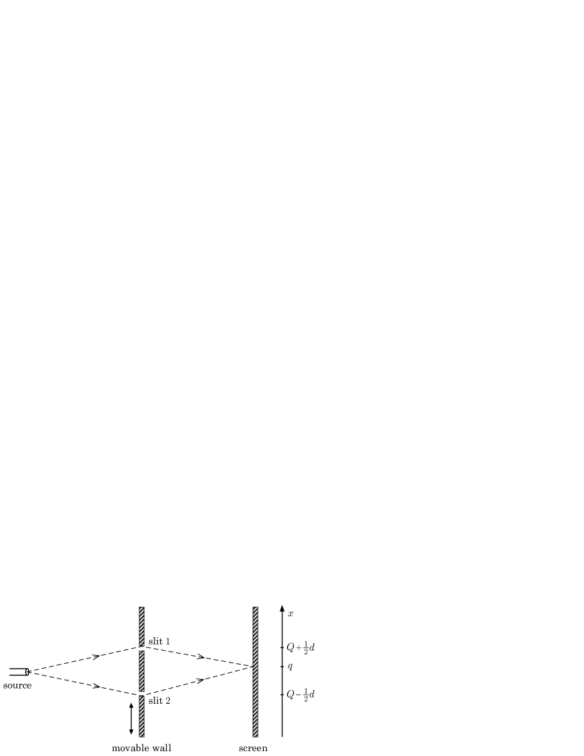
Figure 1: The Young interferometer in the Einstein-Bohr scheme.

The $x$-coordinate of slit 1 is $Q+\frac{d}{2}$ while the $x$-coordinate of slit 2 is $Q-\frac{d}{2}$. A position eigenstate of the whole system is $|q\rangle\otimes|Q\rangle=|q,Q\rangle$. The initial state of the whole system is assumed to be

$$|\mbox{initial}\rangle=|\phi\rangle\otimes|\xi\rangle,$$ (9)

which is a composite of a particle state $|\phi\rangle$ with a wall state $|\xi\rangle$. The emitted particle obeys the free-particle Hamiltonian. Its time-evolution operator is

$$\hat{U}(t)=\exp\Big{(}-\frac{i}{\hbar}\frac{\hat{p}^{2}}{2m}t\Big{)}.$$ (10)

We assume that the particle reaches the slits on the movable wall at the time $\tau$.

The function of the slits are described by two projection operators, $\hat{S}_{1}$ and $\hat{S}_{2}$. If the particle arrives at slit 1, its state becomes $\hat{S}_{1}|\phi\rangle$. If the particle arrives at slit 2, its state becomes $\hat{S}_{2}|\phi\rangle$. They satisfy $\hat{S}_{\alpha}^{\dagger}=\hat{S}_{\alpha}$, $\hat{S}_{\alpha}^{2}=\hat{S}_{\alpha}$, $\hat{S}_{1}+\hat{S}_{2}=1$ and $\hat{S}_{1}\hat{S}_{2}=\hat{S}_{2}\hat{S}_{1}=0$. It is assumed that the particle gives a momentum $+k$ to the wall when the particle hits slit 1. On the other hand, the particle gives a momentum $-k$ to the wall when the particle hits slit 2. This interaction is described by the Hamiltonian

$$\hat{V}=\hat{S}_{1}F(\hat{q}-\hat{Q})-\hat{S}_{2}F(\hat{q}-\hat{Q}).$$ (11)

Here $F$ is a constant force. The evolution operator for an infinitesimal time interval $\Delta t$ is

$$e^{-i\hat{V}\Delta t/\hbar}=e^{-i\hat{S}_{1}k(\hat{q}-\hat{Q})/\hbar\,+\,i\hat{S}_{2}k(\hat{q}-\hat{Q})/\hbar}.$$ (12)

Here $k:=F\Delta t$ is the impact (momentum transfer). The operator $e^{ik\hat{Q}/\hbar}$ shifts the wall momentum as $e^{ik\hat{Q}/\hbar}|P\rangle=|P+k\rangle$ while the operator $e^{-ik\hat{q}/\hbar}$ shifts the particle momentum as $e^{-ik\hat{q}/\hbar}|p\rangle=|p-k\rangle$. Hence, after the momentum exchange, the state of the whole system becomes

$$|\mbox{behind slits}\rangle=e^{-ik\hat{q}/\hbar}\hat{S}_{1}\hat{U}(\tau)|\phi\rangle\otimes e^{ik\hat{Q}/\hbar}|\xi\rangle\,+\,e^{ik\hat{q}/\hbar}\hat{S}_{2}\hat{U}(\tau)|\phi\rangle\otimes e^{-ik\hat{Q}/\hbar}|\xi\rangle.$$ (13)

The particle arrives at the screen at the time $\tau+\tau^{\prime}$. Then the state of the whole system becomes

$$|\mbox{final}\rangle = \hat{U}(\tau^{\prime})e^{-ik\hat{q}/\hbar}\hat{S}_{1}\hat{U}(\tau)|\phi\rangle\otimes e^{ik\hat{Q}/\hbar}|\xi\rangle\,+\,\hat{U}(\tau^{\prime})e^{ik\hat{q}/\hbar}\hat{S}_{2}\hat{U}(\tau)|\phi\rangle\otimes e^{-ik\hat{Q}/\hbar}|\xi\rangle$$ (14)

$$= |\phi_{1}\rangle\otimes e^{ik\hat{Q}/\hbar}|\xi\rangle\,+\,|\phi_{2}\rangle\otimes e^{-ik\hat{Q}/\hbar}|\xi\rangle.$$

Here we put $\hat{U}(\tau^{\prime})e^{-ik\hat{q}/\hbar}\hat{S}_{1}\hat{U}(\tau)|\phi\rangle=|\phi_{1}\rangle$, $\hat{U}(\tau^{\prime})e^{ik\hat{q}/\hbar}\hat{S}_{2}\hat{U}(\tau)|\phi\rangle=|\phi_{2}\rangle$. Then the probability for finding the particle at the position $q$ on the screen is proportional to

$$\mbox{Prob}(q) \propto \int\Big{|}\langle q,Q\,|\mbox{final}\rangle\Big{|}^{2}dQ$$ (15)

$$= \big{|}\phi_{1}(q)\big{|}^{2}+\big{|}\phi_{2}(q)\big{|}^{2}+2\,\mbox{Re}\Big{\{}\phi_{1}^{*}(q)\phi_{2}(q)\,\langle\xi|e^{-2ik\hat{Q}/\hbar}|\xi\rangle\Big{\}}$$

$$= \big{|}\phi_{1}(q)\big{|}^{2}+\big{|}\phi_{2}(q)\big{|}^{2}+2\,{\mathscr{V}}\,\mbox{Re}\Big{\{}e^{i\alpha}\,\phi_{1}^{*}(q)\phi_{2}(q)\Big{\}}.$$

The last term describes an interference of the two waves $\phi_{1}(q)=\langle q|\phi_{1}\rangle$ and $\phi_{2}(q)=\langle q|\phi_{1}\rangle$. The nonnegative real number ${\mathscr{V}}$ and the phase $e^{i\alpha}$ are defined by

$${\mathscr{V}}e^{i\alpha}=\langle\xi|e^{-2ik\hat{Q}/\hbar}|\xi\rangle.$$ (16)

The contrast of the interference fringe is proportional to ${\mathscr{V}}$, which is called the visibility of the interference and takes its value in the range $0\leq{\mathscr{V}}\leq 1$. The wavefunction of the movable wall is denoted as $\xi(Q)=\langle Q|\xi\rangle$ and its Fourier transform is

$$\tilde{\xi}(P)=\frac{1}{\sqrt{2\pi\hbar}}\int e^{-iPQ/\hbar}\,\xi(Q)dQ.$$ (17)

In terms of the wall wavefunctions, the visibility is written as

$${\mathscr{V}}=\left|\int\xi^{*}(Q)\,e^{-2ikQ/\hbar}\,\xi(Q)dQ\right|=\left|\int\tilde{\xi}^{*}(P-k)\,\tilde{\xi}(P+k)dP\right|.$$ (18)

After observing the position of the particle on the screen, we measure the momentum of the wall to detect the path of the particle. The conditional probability distribution of the momentum $P$ is calculated from (14) as

$$\mbox{Prob}(P|q)\>\propto\>\Big{|}\langle q,P\,|\mbox{final}\rangle\Big{|}^{2}=\left|\phi_{1}(q)\,\tilde{\xi}(P-k)+\phi_{2}(q)\,\tilde{\xi}(P+k)\right|^{2}.$$ (19)

If the support of the initial wavefunction $|\tilde{\xi}(P)|$ is contained within the range $P_{0}-k<P<P_{0}+k$ for some $P_{0}$, then from the measured value of $P$ we can tell the slit which the particle passed. Namely, if the measured momentum is in the range $P_{0}<P<P_{0}+2k$, we can say that the particle hit slit 1. On the other hand, if the measured momentum is in the range $P_{0}-2k<P<P_{0}$, we can say that the particle hit slit 2. However, if the support of $|\tilde{\xi}(P)|$ is contained within $P_{0}-k<P<P_{0}+k$, the overlap integral in (18) vanishes and hence the interference fringes fade away completely.

Contrarily, if the width of the support of $\tilde{\xi}(P)$ is larger than $2k$, the visibility (18) can be nonzero. However, at that time, the probability (19) can have a nonzero interference term and hence we cannot distinguish the particle path certainly.

We summarize the above argument symbolically as

Visible interference $$\Leftrightarrow {\mathscr{V}}\neq 0$$

$$\Rightarrow \mbox{supp}\,|\tilde{\xi}(P-k)|\cap\mbox{supp}\,|\tilde{\xi}(P+k)|\;\;\mbox{has nonzero measure}.$$

$$\Leftrightarrow$$ The path of the particle cannot be distinguished completely

by measuring the momentum of the wall.

In the above inference, the second arrow $(\Rightarrow)$ cannot be replaced with the necessary and sufficient sign $(\Leftrightarrow)$. For example, if we take the wavefunction

$$\tilde{\xi}(P)=\left\{\begin{array}[]{ll}a\,\sin\left(\frac{2\pi P}{2k}\right)&(0\leq P\leq 2k)\\ b\,\sin\left(\frac{4\pi P}{2k}\right)&(-2k\leq P\leq 0)\\ 0&(\mbox{otherwise}),\end{array}\right.$$ (20)

then the supports of $|\tilde{\xi}(P-k)|$ and $|\tilde{\xi}(P+k)|$ have an overlap with nonzero measure but the integral ${\mathscr{V}}$ vanishes.

3 Uncertainty relation

Now we discuss what kind of uncertainty relation is involved in the double-slit experiment. Let us consider the expression (18) for the visibility,

$${\mathscr{V}}(k)=\left|\int e^{-2ikQ/\hbar}\,|\xi(Q)|^{2}\,dQ\right|.$$ (21)

Suppose that the probability distribution $|\xi(Q)|^{2}$ has an effective width $\Delta Q$. (A rigorous definition of $\Delta Q$ is not necessary for the following argument.) Since (21) is an oscillatory integral, to get a considerably large visibility we need to have

$$2k\,\Delta Q/\hbar\>\lesssim\>2\pi.$$ (22)

On the other hand, as discussed above, to distinguish the slit which the particle passes, the initial momentum distribution of the double-slit wall should be contained within the range

$$\Delta P<2k.$$ (23)

Hence, to observe a clear interference and to distinguish the path of the particle simultaneously, we need to have

$$\Delta Q\,\Delta P\>\lesssim\>2\pi\hbar.$$ (24)

As a contraposition, the uncertainty relation

$$\Delta Q\,\Delta P\>\gtrsim\>2\pi\hbar$$ (25)

implies that exhibiting a clear interference pattern and detecting the particle path cannot be accomplished simultaneously. This uncertainty relation (25) is a property of the initial state of the double-slit wall but it is not a relation between error and disturbance caused by measurement. Hence, we conclude that the obstruction against the simultaneous realization of interference and path detection is the Kennard-type uncertainty relation which is intrinsic to the quantum state of the double-slit wall. This is the main claim of this paper. It is to be noted that this is a conclusion of an analysis of the specific model. We do not have to take it as a universally valid statement.

It is a long-standing issue whether the position-momentum uncertainty relation does imply or not the particle-wave complementarity. Storey et al. [20, 21] argued that the position-momentum uncertainty relation is responsible for destroying the interference pattern. Englert et al. [22, 23] took an opposite position and argued that the which-way information is responsible for destroying the interference pattern. Dürr, Nonn, and Rempe [24, 25] performed experiments to prove that what destroys the interference pattern is the which-way information. Hence, Englert’s argument seems to be correct. However, momentum disturbance is still necessary for the change of the interference pattern in the which-way experiment, and Englert did not answer to this point.

What we discussed in this paper is a question asking which kind of the position-momentum uncertainty relation is responsible for destroying the interference pattern when we try to detect the path of the particle by measuring the momentum of the movable slit-wall. Our answer is that the Kennard-type uncertainty relation is responsible in the context of our model.

4 Suggestions for experiments

Here we would like to suggest an experimental scheme to test the visibility relation (18). Our scheme uses the Michelson interferometer as illustrated in Fig. 2. A photon is emitted from a light source (a) and is split by a beam splitter (b) into two directions. At the end (c) of one direction, an atom or a molecule is placed. The incident photon is scattered by the atom and the atom recoils. At the other end (d) a mirror is fixed. The two paths merge at the beam splitter (b) and the photon reaches the fixed screen (e). There we observe an interference pattern by accumulating photons. On the other hand, by measuring the velocity of the atom, we can infer the path of the photon; If the atom recoils out, we know that the photon took the path (c). If the atom remains stationary, we know that the photon took the path (d).

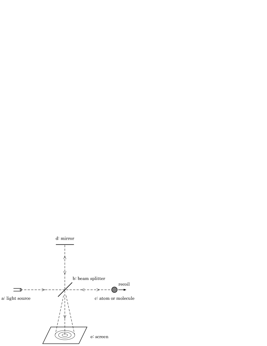
Figure 2: The Michelson interferometer.

If the initial wavefunction of the atom is strongly localized, one will observe a clear interference pattern but fail to determine the velocity of the atom precisely. If the initial wavefunction of the atom has a larger spatial spread, one can determine the velocity of the atom with a smaller error but the interference pattern will become feebler. Thus the initial state of the atom defines the visibility of the interference fringe as (18). We may put a Bose-Einstein condensate (BEC) of atoms at the place (c) instead of a single atom since control and observation of the BEC are more feasible than a single atom.

We can estimate the velocity of the recoiling atom. It is assumed that the photon has wave length $\lambda$ and the target atom has mass $M$. Then the photon momentum is $p=h/\lambda$ and the impact given to the atom is $k=2p$. The velocity of the recoil atom is

$$v=\frac{k}{M}=\frac{2h}{M\lambda}.$$ (26)

Assume that the photon wave length is $\lambda=0.5\times 10^{-6}$ m and that we use a mercury atom as a reflector. Then the recoil velocity is $v=7.9\times 10^{-3}\,{\rm m}\cdot{\rm s}^{-1}$. If we use a BEC of $10^{4}$ sodium atoms, the velocity is $v=6.9\times 10^{-6}\,{\rm m}\cdot{\rm s}^{-1}$. On the other hand, the argument around Eq. (22) implies that the size of the spread of the wavefunction of the target should be smaller than

$$\Delta Q\sim\frac{\pi\hbar}{k}=\frac{1}{4}\lambda$$ (27)

for exhibiting a clear interference pattern.

In the above argument we proposed a use of the Michelson interferometer. Other interference experiments, like the Hanbury-Brown-Twiss correlation [26, 27] or the interference of photons from two light sources, which has been demonstrated by Mandel et al. [28, 29], can also be modified to experiments which demonstrate the tradeoff between interference and distinguishability. It is also to be noted that Plau et al. [30] and Chapman et al. [31] had demonstrated that a change of the momentum distribution of an atom by photon emission or by photon scattering causes a change of spatial coherence of the atom. They had confirmed the Kennard-type uncertainty relation.

After completing this manuscript, we have learned that a group of Miron [19] successfully observed interference pattern of electrons emitted from two atoms. They observed also disappearance of the interference fringes when the atoms were not fixed and the atom emitting an electron recoiled by the momentum transfer.

5 Entanglement as a root of measurement effects

Various phenomena including distinguishability, interference and decoherence, quantum eraser, and weak value, which occur at the interface between quantum systems and classical systems, are related to measurement and entanglement. Before closing our discussion we would like to explain that these phenomena can be understood on the same footing.

Assume that an object system is in a superposed state $c_{1}|\phi_{1}\rangle+c_{2}|\phi_{2}\rangle$ and an apparatus is in a state $|\xi\rangle$. The vectors $|\phi_{1}\rangle$, $|\phi_{2}\rangle$ are unit vectors, but not necessarily orthogonal. The initial state of the whole system is the tensor product state

$$\Big{(}c_{1}|\phi_{1}\rangle+c_{2}|\phi_{2}\rangle\Big{)}\otimes|\xi\rangle.$$ (28)

Interaction between the object and the apparatus entangles the two systems to the state

$$|\Psi\rangle=\hat{U}\Big{(}c_{1}|\phi_{1}\rangle+c_{2}|\phi_{2}\rangle\Big{)}\otimes|\xi\rangle=c_{1}|\phi_{1}\rangle\otimes|\xi_{1}\rangle+c_{2}|\phi_{2}\rangle\otimes|\xi_{2}\rangle.$$ (29)

It is assumed that the vectors $|\xi_{1}\rangle$, $|\xi_{2}\rangle$ are unit vectors, but not necessarily orthogonal. The object has an observable $\hat{A}$ and the apparatus has an observable $\hat{M}$. The spectral decompositions of these observables are

$$\hat{A}=\sum_{a}a\,\hat{P}_{A}(a),\qquad\hat{M}=\sum_{m}m\,\hat{P}_{M}(m).$$ (30)

In the followings, we explain that various aspects of measurement can be understood as properties of the entangled state (29).

i) Which-way distinguishability: In the context of which-way experiment, the apparatus is designed for distinguishing the object states $|\phi_{1}\rangle$ and $|\phi_{2}\rangle$. After the interaction, the probability for reading out the value $m$ from the meter observable $\hat{M}$ is given by

$$\mbox{Prob}(\hat{M}=m) = \langle\Psi|\hat{P}_{M}(m)|\Psi\rangle$$ (31)

$$= |c_{1}|^{2}\langle\xi_{1}|\hat{P}_{M}(m)|\xi_{1}\rangle+|c_{2}|^{2}\langle\xi_{2}|\hat{P}_{M}(m)|\xi_{2}\rangle$$

$$\,+\,2\,\mbox{Re}\,\big{\{}c_{1}^{*}c_{2}\,\langle\phi_{1}|\phi_{2}\rangle\,\langle\xi_{1}|\hat{P}_{M}(m)|\xi_{2}\rangle\big{\}}.$$

If the third term $\langle\phi_{1}|\phi_{2}\rangle\,\langle\xi_{1}|\hat{P}_{M}(m)|\xi_{2}\rangle$ vanishes, and if either $\langle\xi_{1}|\hat{P}_{M}(m)|\xi_{1}\rangle$ or $\langle\xi_{2}|\hat{P}_{M}(m)|\xi_{2}\rangle$ vanishes, we successfully distinguish the states $|\phi_{1}\rangle$ and $|\phi_{2}\rangle$ by reading the value $m$. Oppositely, if the both terms $\langle\xi_{1}|\hat{P}_{M}(m)|\xi_{1}\rangle$ and $\langle\xi_{2}|\hat{P}_{M}(m)|\xi_{2}\rangle$ are nonzero, we have error for distinguishing the states $|\phi_{1}\rangle$ and $|\phi_{2}\rangle$. If the third term $\langle\phi_{1}|\phi_{2}\rangle\,\langle\xi_{1}|\hat{P}_{M}(m)|\xi_{2}\rangle$ is nonzero, the distinguishing measurement fails, too. When the meter states $|\xi_{1}\rangle$ and $|\xi_{2}\rangle$ are orthogonal, the meter becomes optimal for distinguishing the states $|\phi_{1}\rangle$ and $|\phi_{2}\rangle$.

ii) Interference visibility and decoherence: If we measure the quantity $\hat{A}$ directly, the probability for obtaining the value $a$ of $\hat{A}$ is

$$\mbox{Prob}(\hat{A}=a) = \langle\Psi|\hat{P}_{A}(a)|\Psi\rangle$$ (32)

$$= |c_{1}|^{2}\langle\phi_{1}|\hat{P}_{A}(a)|\phi_{1}\rangle+|c_{2}|^{2}\langle\phi_{2}|\hat{P}_{A}(a)|\phi_{2}\rangle$$

$$\,+\,2\,\mbox{Re}\,\big{\{}c_{1}^{*}c_{2}\,\langle\phi_{1}|\hat{P}_{A}(a)|\phi_{2}\rangle\,\langle\xi_{1}|\xi_{2}\rangle\big{\}}.$$

The interference effect is characterized by the coefficient $c_{1}^{*}c_{2}$, which depends on the phases of $c_{1}$ and $c_{2}$. When the matrix element $\langle\phi_{1}|\hat{P}_{A}(a)|\phi_{2}\rangle$ is nonzero, the interference effect is observed. But the contrast of interference fringe is reduced by the factor $\langle\xi_{1}|\xi_{2}\rangle$. When the meter states $|\xi_{1}\rangle$ and $|\xi_{2}\rangle$ is orthogonal, the which-way distinguishing measurement is optimized but the interference effect is completely lost.

iii) Quantum eraser: The above argument tells that the distinguishability is maximized but the interference effect is lost when $\langle\xi_{1}|\xi_{2}\rangle=0$. However, even when $\langle\xi_{1}|\xi_{2}\rangle=0$, by a joint measurement of $\hat{A}$ and $\hat{M}$ the interference effect is recovered. The joint probability for observing the values $\hat{A}=a$ and $\hat{M}=m$ is

$$\mbox{Prob}(\hat{A}=a,\hat{M}=m) = |c_{1}|^{2}\langle\phi_{1}|\hat{P}_{A}(a)|\phi_{1}\rangle\langle\xi_{1}|\hat{P}_{M}(m)|\xi_{2}\rangle$$ (33)

$$\,+\,|c_{2}|^{2}\langle\phi_{2}|\hat{P}_{A}(a)|\phi_{2}\rangle\langle\xi_{1}|\hat{P}_{M}(m)|\xi_{2}\rangle$$

$$\,+\,2\,\mbox{Re}\,\big{\{}c_{1}^{*}c_{2}\,\langle\phi_{1}|\hat{P}_{A}(a)|\phi_{2}\rangle\,\langle\xi_{1}|\hat{P}_{M}(m)|\xi_{2}\rangle\big{\}}.$$

Note that $\langle\xi_{1}|\hat{P}_{M}(m)|\xi_{2}\rangle$ can be nonzero even when $\langle\xi_{1}|\xi_{2}\rangle=0$. Thus the interference effect is observed by the joint measurement of $\hat{A}$ and $\hat{M}$ although the interference effect is not observed by the measurement of $\hat{A}$ alone. However, the which-way distinguishability is reduced as $\langle\xi_{1}|\hat{P}_{M}(m)|\xi_{2}\rangle\neq 0$. In a sense, the which-way information is erased for reviving the interference fringe, and hence this effect is named quantum eraser. The conditional probability for obtaining the value $a$ of $\hat{A}$ under the restriction $\hat{M}=m$ is calculated as

$$\mbox{Prob}(\hat{A}=a|\hat{M}=m) = \frac{\mbox{Prob}(\hat{A}=a,\hat{M}=m)}{\mbox{Prob}(\hat{M}=m)}.$$ (34)

iv) Weak value: The weak probability is the conditional probability for obtaining the meter value $m$ of $\hat{M}$ under the selection of object value $\hat{A}=a$,

$$\mbox{Prob}(\hat{M}=m|\hat{A}=a) = \frac{\mbox{Prob}(\hat{A}=a,\hat{M}=m)}{\mbox{Prob}(\hat{A}=a)}.$$ (35)

When the probability $\mbox{Prob}(\hat{A}=a)$ is small, that means the measurement disturbance is small, the joint probability $\mbox{Prob}(\hat{M}=m|\hat{A}=a)$ becomes large. Thus a kind of enhancement or amplification of the meter value can occur. This is mechanism of the so-called weak measurement.

Before summarizing our discussion, we give a brief overview of the developments in this area. Englert [32] formulated a qualitative relation between distinguishability and interference visibility. Dürr and Rempe [33] gave a general proof of the Englert formula using the noncommutativity of observables. Dürr et al. [25] tested this formula by experiment. Hosoya et al. [34] investigated the complementarity of which-way distinguishability and interference from the viewpoint of entanglement.

Scully and Drühl [35] introduced the idea of quantum eraser. Experimental realization of quantum eraser have been achieved repeatedly, for example, as demonstrated by Hillmer and Kwiat [36].

Aharonov, Albert and Vaidman [37] introduced the idea of weak value as an extended notion of the values of physical observables. The weak value is a value of meter conditioned by a postselected object value. It was first pointed out by Tamate et al. [38] that the structure of the weak value (35) is dual to the structure of the quantum eraser (34).

6 Summary

In this paper we analyzed the double-slit scheme that exhibits the interference pattern on the screen and distinguishes the path of a particle by measuring momentum of the wall. This double-slit setting has an entangled state of the particle and the wall. Finally, we concluded that the Kennard-type uncertainty relation of fluctuations of position and momentum of the wall is a reason of the complementarity in the double-slit experiment. Similar analysis has been done by Qureshi and Vathsan [39]. It is also to be noted Busch and Shilladay presented a study of the complementarity in Mach-Zehnder interferometry [40].

References

- [1] W. Heisenberg, Uber den anschaulichen Inhalt der quantentheoretischen Kinematik und Mechanik, Z. Phys. 43, 172 (1927).
- [2] W. Heisenberg, The Physical Principles of the Quantum Theory, English translation by C. Eckart and F. C. Hoyt (University of Chicago Press, 1930; Dover, 1949).
- [3] J. von Neumann, Die mathematische Grundlagen der Quantenmechanik (Springer, 1932); Mathematical Foundations of Quantum Mechanics (Princeton University Press, 1996).
- [4] E. H. Kennard, Zur Quantenmechanik einfacher Bewegungstypen, Z. Phys. 44, 326 (1927).
- [5] H. P. Robertson, The uncertainty principle, Phys. Rev. 34, 163 (1929).
- [6] V. B. Braginskii and Yu. I. Vorontsov, Quantum-mechanical limitations in macroscopic experiments and modern experimental technique, Soviet Physics Usp. 17, 644 (1975).
- [7] C. M. Caves, K. S. Thorne, R. W. P. Drever, V. D. Sandberg, and M. Zimmermann, On the measurement of a weak classical force coupled to a quantum-mechanical oscillator. I. Issues of principle, Rev. Mod. Phys. 52, 341 (1980).
- [8] H. P. Yuen, Contractive states and the standard quantum limit for monitoring free-mass positions, Phys. Rev. 51, 719 (1983).
- [9] C. M. Caves, Defense of the standard quantum limit for free-mass position, Phys. Rev. Lett. 54, 2465 (1985).
- [10] M. Ozawa, Measurement breaking the standard quantum limit for free-mass position, Phys. Rev. Lett. 60, 385 (1988).
- [11] J. Maddox, Beating the quantum limits, Nature 331, 559 (1988).
- [12] M. Ozawa, Physical content of Heisenberg’s uncertainty relation: limitation and reformulation, Phys. Lett. A 318, 21 (2003).
- [13] M. Ozawa, Quantum measuring processes of continuous observables, J. Math. Phys. 25, 79 (1984).
- [14] M. Ozawa, Uncertainty relations for noise and disturbance in generalized quantum measurements, Ann. Phys. 311, 350 (2004).
- [15] C. Branciard, Error-tradeoff and error-disturbance relations for incompatible quantum measurements, PNAS 110, 6742 (2013).
- [16] N. Bohr, Discussion with Einstein on epistemological problems in atomic physics, in Quantum Theory and Measurement (eds. J. A. Wheeler and W. H. Zurek) pp. 9-49 (Princeton University Press, 1983).
- [17] A. Messiah, Quantum Mechanics, translated from French by G. M. Temmer, Chap. 4, Sec. 18 (North-Holland, 1961; Dover, 1999).
- [18] R. P. Feynman, R. B. Leighton, and M. Sands, The Feynman Lectures on Physics, Vol. 3, Secs. 1-8, 3-1, 3-2 (Addison-Wesley, 1966).
- [19] X.-J. Liu, Q. Miao, F. Gel’mukhanov, M. Patanen, O. Travnikova, C. Nicolas, H. Ågren, K. Ueda, and C. Miron, Einstein-Bohr recoiling double-slit gedanken experiment performed at the molecular level, Nature Photonics 9, 120 (2015)
- [20] P. Storey, S. Tan, M. Collett, and D. Walls, Path detection and the uncertainty principle, Nature 367, 626 (1994).
- [21] P. Storey, S. Tan, M. Collett, and D. Walls, Complementarity and uncertainty, Nature 375, 368 (1995).
- [22] M. O. Scully, B.-G. Englert, and H. Walther, Quantum optical tests of complementarity, Nature 351, 111 (1991).
- [23] B.-G. Englert, M. O. Scully, and H. Walther, Complementarity and uncertainty, Nature 375, 367 (1995).
- [24] S. Dürr, T. Nonn, and G. Rempe, Origin of quantum-mechanical complementarity probed by a ‘which-way’ experiment in an atom interferometer, Nature 395, 33 (1998).
- [25] S. Dürr, T. Nonn, and G. Rempe, Fringe visibility and which-way information in an atom interferometer, Phys. Rev. Lett. 81, 5705 (1998).
- [26] R. Hanbury Brown and R. Q. Twiss, Correlation between photons in two coherent beams of light, Nature 177, 27 (1956);
- [27] R. Hanbury Brown and R. Q. Twiss, A test of a new type of stellar interferometer on Sirius, Nature 178, 1046 (1956).
- [28] G. Magyar and L. Mandel, Interference fringes produced by superposition of two independent maser light beams, Nature 198, 255 (1963).
- [29] L. Mandel, Quantum effects in one-photon and two-photon interference, Rev. Mod. Phys. 71, S274 (1999).
- [30] T. Pfau, S. Spälter, Ch. Kurtsiefer, C. R. Ekstrom, and J. Mlynek, Loss of spatial coherence by a single spontaneous emission, Phys. Rev. Lett. 73, 1223 (1994).
- [31] M. S. Chapman, T. D. Hammond, A. Lenef, J. Schmiedmayer, R. A. Rubenstein, E. Smith, and D. E. Pritchard, Photon scattering from atoms in an atom interferometer: Coherence lost and regained, Phys. Rev. Lett. 75, 3783 (1995).
- [32] B.-G. Englert, Fringe visibility and which-way information: an inequality, Phys. Rev. Lett. 77, 2154 (1996).
- [33] S. Dürr and G. Rempe, Can wave-particle duality be based on the uncertainty relation?, Am. J. Phys. 68, 1021 (2000).
- [34] A. Hosoya, A. Carlini, and S. Okano, Complementarity of entanglement and interference, Int’l J. Mod. Phys. C 17, 493 (2006).
- [35] M. O. Scully and K. Drühl, Quantum eraser: A proposed photon correlation experiment concerning observation and “delayed choice” in quantum mechanics, Phys. Rev. A 25, 2208 (1982).
- [36] R. Hillmer and P. Kwiat, A do-it-yourself quantum eraser, Sci. Am. 5, 72 (2007).
- [37] Y. Aharonov, D. Z. Albert, and L. Vaidman How the result of a measurement of a component of the spin of a spin-1/2 particle can turn out to be 100, Phys. Rev. Lett. 60, 1351 (1988).
- [38] S. Tamate, H. Kobayashi, T. Nakanishi, K. Sugiyama, and M. Kitano, Geometrical aspects of weak measurements and quantum erasers, New J. Phys. 11, 093025 (2009).
- [39] T. Qureshi and R. Vathsan, Einstein’s recoiling slit experiment, complementarity and uncertainty, Quanta 2, 58 (2013).
- [40] P. Busch and C. Shilladay, Complementarity and uncertainty in Mach-Zehnder interferometry and beyond, Phys. Rep. 435, 1 (2006).