Coherent control of photon propagation
via electromagnetically induced transparency in lossless media

Abstract

We study the influence of a lossless material medium on the coherent storage and quantum state transfer of a quantized probe light in an ensemble of $\Lambda$-type atoms. The medium is modeled as uniformly distributed two-level atoms with same energy level spacing, coupling to a probe light. This coupled system can be simplified to a collection of two-mode polaritons which couple to one transition of the $\Lambda$-type atoms. We show that, when the other transition of $\Lambda$-type atoms is controlled by a classical light, the electromagnetically induced transparency can also occur for the polaritons. In this case the coherent storage and quantum transfer for photon states are achievable through the novel dark states with respect to the polaritons. By calculating the corresponding dispersion relation, we find the ensemble of the three-level atoms with $\Lambda$-type transitions may serve as quantum memory for it slows or even stops the light propagation through the mechanism of electromagnetically induced transparency.

I Introduction

Electromagnetically induced transparency (EIT) harris is a typical quantum coherent effect, in which the propagation of probe a field in a $\Lambda$-type atom ensemble can be well controlled by a classical light hau ; Kash . Most recently, the EIT phenomenon was suggested as an active mechanism Lukin1 ; Lukin2 ; Lukin3 to slow down and even stop the photon propagation, so that the photon state can be stored or released coherently. These investigations Lukin1 ; Lukin2 ; Lukin3 are mainly motivated by the fast development of quantum information science and technology Zei . This is because, with the help of quantum storage, one could complete a series of quantum logical operations within the decoherence time.

In this paper we study the EIT mechanism for quantum information processing in the presence of a lossless medium. This is motivated by two reasons. Firstly, we notice that buffer gases, with different atom species, are used in some of the recent EIT experiments buffer1 ; buffer2 . Usually one introduces a buffer gas to lengthen the ground-state coherence lifetime of confined EIT atoms. For the EIT effect in a $\Lambda$–sample with a buffer gas, the probe field has a low group velocity when it has a small detuning with respect to resonance buffer1 ; buffer2 . These coherent phenomena essentially result from the gaseous medium : the buffer gas. To see the coherent effect of the buffer gas, one sets up atoms in the “buffer gas” to be resonant with the probe light (in this case the “buffer gas” no longer only acts as a buffer to cool down the EIT atoms ), the “buffer gas” just plays the role of a coherent medium; that the photon will be coupled with collective excitations of the buffer atoms to form quasi-particles, called polaritons.

Secondly, the study of EIT for photon state storage should be extended to solid state systems for applications in scalable quantum computing. Here, EIT atoms with $\Lambda$-type transitions may be realized using solid state devices, such as artificial atoms based on quantum dots, which are usually embedded in a solid state substrate. To make such solid state devices as coherent storage units based on the EIT mechanism, one should consider the EIT process in the medium of the substrate.

In our study, we first model the medium as a collection of $N$ two-level atoms, weakly coupled to the quantized probe field Dutra . The “weak” interaction between the atoms and the probe field is assumed to excite a few atoms, such that the collective excitations of the atoms behave as bosons. In turn, the photons of the probe field are dressed by the collective excitations, forming polaritons hopfield of two modes. According to Hopfield’s original paper on quantum polariton hopfield and also according to others Dutra  , such polariton can be regarded as a macroscopically averaged electromagnetic field or a displacement field.

We then show that, when one of the two polariton modes is resonant with the three-level $\Lambda$-type atoms, there still exists a dark state which decouples from the upper energy level of the $\Lambda$-atom. Utilizing the dark state, we can adiabatically manipulate the quantum state of the photon such that the photon state is coherently transferred to the atomic collective excitation state. We further calculate the susceptibility of the light propagation in the EIT atomic ensemble embedded in a medium.

In usual case, due to inhomogeneous broadening, ground state decoherence, loss, etc, the broaden energy levels of atoms in the EIT ensemble can behave as energy bands and thus limit the transparency due to the off-resonance of some atoms. Here, the coherent processes induced by the two-level lossless medium can only results in a frequency split of effective light field, which also causes the off-resonance with respect to the fixed energy levels of EIT atoms. However, by making use of the Hopfield model hopfield ; Dutra , the split can be estimated quantitatively and then one can restore the resonance for the EIT by the effective light filed in the medium.

The remaining part of this paper is organized as follows. In Sec. II, we study the coupled system of quantum light plus medium atoms, and describe this using two-mode polaritons. Section II is devoted to study the EIT effect of a single three-level atom induced by polaritons. In Sec. IV, for an ensemble of three-level atoms, we construct the many-atom dark states based on the spectra-generating algebra method. The influence of the medium on quantum state transfer is discussed in Sec. V. In Sec. VI, we study the propagation of dressed light. Finally, conclusions are presented in Sec. VII.

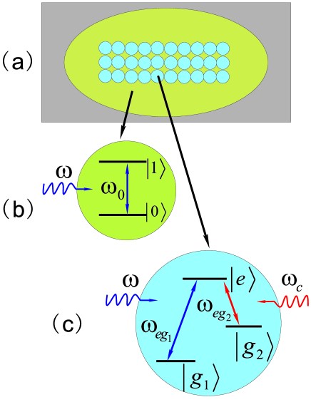
Figure 1: (Color online) (a) Schematic diagram of the system under consideration. (b) The medium [yellow background in (a)] is modeled by $N$ two-level atoms, each medium atom has an identical transition frequency $\omega_{0}$. (c) The level structure of the three-level $\Lambda$-type atoms.

II Microscopic Hopfield model for material media interacting with a single-mode cavity field

The system under consideration, shown schematically in Fig. 1, includes a single-mode cavity, a lossless medium, and $M$ identical three-level $\Lambda$-type atoms. The medium is modeled by $N$ two-level atoms with equal level spacing $\omega_{0}$, and for the $j$th medium atom, the ground and excited states are denoted, respectively, as $|0\rangle_{j}$ and $|1\rangle_{j}$. The three-level $\Lambda$-type atoms have two lower states $|g_{1}\rangle$ and $|g_{2}\rangle$ plus an upper state $|e\rangle$. A single-mode cavity field $\omega$ is assumed as the probe field to induce a transition between levels $|e\rangle$ and $|g_{1}\rangle$. Finally, a classical control field $\omega_{c}$ is introduced to couple $|e\rangle$ and $|g_{2}\rangle$.

To better understand the effect of the medium, we shall only consider, in this section, the interaction between the single-mode probe field and the medium, which is described by the Hamiltonian

$$H_{\text{L-M}} =\hbar\omega a^{{\dagger}}a+\hbar\omega_{0}\sum_{j=1}^{N}\left|1\right\rangle_{j}\left\langle 1\right|$$

$$+\hbar\sum_{j=1}^{N}g_{j}\left(a+a^{{\dagger}}\right)\left(\sigma_{+}^{\left(j\right)}+\sigma_{-}^{\left(j\right)}\right),$$ (1)

where $a^{{\dagger}}$ ($a$) is the creation (annihilation) operator for the quantum probe field, $\sigma_{+}^{\left(j\right)}=\left|1\right\rangle_{j}\left\langle 0\right|$, $\sigma_{-}^{\left(j\right)}=\left|0\right\rangle_{j}\left\langle 1\right|$, and $\sigma_{z}^{\left(j\right)}=\left|1\right\rangle_{j}\left\langle 1\right|-\left|0\right\rangle_{j}\left\langle 0\right|$ are the quasi-spin Pauli operators for the $j$th atom. Here $g_{j}$ is the electric-dipole coupling strength between the probe field and the $j$th atom. For simplicity, we shall assume throughout this paper that $g_{j}\equiv g_{\text{medium}}$ is independent of individual atom.

To simplify Hamiltonian (1), we define the collective quasi-spin wave operators as

$$B_{k}^{\dagger} =\frac{1}{\sqrt{N}}\sum_{j=1}^{N}\sigma_{+}^{\left(j\right)}\exp\left(\frac{2\pi ikj}{N}\right),$$

$$B_{k} =\frac{1}{\sqrt{N}}\sum_{j=1}^{N}\sigma_{-}^{\left(j\right)}\exp\left(-\frac{2\pi ikj}{N}\right),$$

where $k=0,\,\cdots,\,N-1$. In the large–$N$ limit with low excitation condition, it was proven that the above collective quasi-spin wave operators $B_{k}$ and $B_{k^{\prime}}^{\dagger}$ satisfy the bosonic commutation relations Sun ; Jin

$$\left[B_{k},B_{k^{\prime}}^{\dagger}\right]=\delta_{kk^{\prime}}\,,$$ (2)

and

$$\sum_{j=1}^{N}\,\left|1\right\rangle_{j}\left\langle 1\right|=\sum_{k}B_{k}^{{\dagger}}\,B_{k}.$$

The commutation relation in Eq. (2) suggests that the low-excitation behavior of the medium can be described by $N$ bosonic operators, i.e., exciton operators. The low energy part of Eq. (1) then reduces to Hopfield’s Hamiltonian hopfield

$$H_{\text{L-M}}=\hbar\omega a^{{\dagger}}a+\hbar\omega_{0}B_{0}^{{\dagger}}B_{0}+\hbar G\left(a+a^{{\dagger}}\right)\left(B_{0}+B_{0}^{{\dagger}}\right),$$ (3)

where $G=g_{\text{medium}}\,\sqrt{N}\,\propto\sqrt{N/V}$, with $V$ being the effective volume of the probe field, has a finite van Hove limit. We remark that, to obtain Eq. (3), we have neglected $N-1$ free exciton modes $B_{1},\,B_{2},\,\cdots,\,B_{N-1}$, as they are decoupled from the probe field.

Equation (3) can be solved using polariton operators employed by several authors hopfield ; Dutra . Following the procedure given in Ref. Dutra , we define the polariton operators as

$$c_{k}=x_{1}^{k}a+y_{1}^{k}a^{{\dagger}}+x_{2}^{k}B_{0}+y_{2}^{k}B_{0}^{{\dagger}}$$ (4)

with $k=1,\,2$. $c_{k}$ and $c_{k^{\prime}}^{{\dagger}}$ satisfy the usual bosonic commutation relation $\left[c_{k},c_{k^{\prime}}^{{\dagger}}\right]=\delta_{k,k^{\prime}}$ and $\left[c_{k},c_{k^{\prime}}\right]=0$. Assuming that the Hamiltonian Eq. (3) is diagonalized by $c_{1}$ and $c_{2}$, namely,

$$H_{\text{L-M}}=\hbar\Omega_{1}c_{1}^{{\dagger}}c_{1}+\hbar\Omega_{2}c_{2}^{{\dagger}}c_{2},$$

the coefficients $x_{l}^{k}$ and $y_{l}^{k}$ $(l,\,k=1,\,2)$ are then obtained via equations

$$\left[c_{k},H_{\text{L-M}}\right]\,=\,\hbar\,\Omega\,c_{k}.$$

Explicitly, we have

$$x_{j}^{k}=\frac{1}{2}\left(v_{j}^{k}+u_{j}^{k}\right),\,y_{j}^{k}=\frac{1}{2}\left(v_{j}^{k}-u_{j}^{k}\right),\,\,$$

where

$$u_{1}^{k} =\frac{\omega}{\Omega_{k}}v_{1}^{k},\,\,\,\,\,\,\,\,\,\,\,\,\,\,\,u_{2}^{k}=\frac{\Omega_{k}^{2}-\omega^{2}}{2G\Omega_{k}}v_{2}^{k},$$

$$\,v_{2}^{k} =\frac{\Omega_{k}^{2}-\omega^{2}}{2G\omega_{0}}v_{1}^{k},\,v_{1}^{k}=\sqrt{\frac{4G^{2}\Omega_{k}\omega_{0}}{\left(\Omega_{k}^{2}-\omega^{2}\right)^{2}+4\omega_{0}\omega G^{2}}}\,,$$

and the eigenfrequencies

$$\Omega_{k}^{2}=\frac{1}{2}\left\{\omega_{0}^{2}+\omega^{2}+\left(-1\right)^{k}\sqrt{\left(\omega_{0}^{2}-\omega^{2}\right)^{2}+16\omega\,\omega_{0}\,G^{2}}\right\}.$$ (5)

The above results are identical to those obtained using the Hopfield’s approach, as shown in Ref. hopfield , where the effect of the medium is phenomenologically modeled by many harmonic oscillators. Our results then indicate that those phenomenological harmonic oscillators essentially originate from the low-energy collective excitations of the medium atoms. As a matter of fact, same as the previous treatments for the effect of the medium  Dutra , our approach also relies on the weak-coupling assumption, which suggests that the medium effect can be equivalently studied according to either the two-level model or the harmonic oscillators.

III Effect of material media on the dark state of a three-level atom

In this section, we shall assume that there is only one three-level $\Lambda$-type atom embedded in the medium. As explained in Sect. II, this atom couples with a single-mode cavity field and a classical light field. However, due to the effect of the medium, the single cavity mode is effectively replaced by the two-mode polariton, resulting in the two-color EIT model shown in Fig. 2. The corresponding Hamiltonian takes the form

$$h = \hbar\sum_{i=1}^{2}\Omega_{i}c_{i}^{{\dagger}}c_{i}+\hbar\,\omega_{eg_{1}}\left|e\right\rangle\left\langle e\right|+\hbar\left(\omega_{eg_{1}}-\omega_{eg_{2}}\right)\left|g_{2}\right\rangle\left\langle g_{2}\right|$$ (6)

$$+\hbar g\sum_{i=1}^{2}u_{i}\left(c_{i}+c_{i}^{{\dagger}}\right)\left(\left|e\right\rangle\left\langle g_{1}\right|+\mathrm{h.c.}\right)$$

$$+\hbar\,\xi\left(e^{-i\omega_{c}t}\left|e\right\rangle\left\langle g_{2}\right|+\mathrm{h.c.}\right),$$

where $u_{i}=u_{1}^{i}$, $g$ and $\xi$ are the Rabi-frequencies for, respectively, the single-mode cavity field and the classical light field, and $\omega_{eg_{1}}$ ($\omega_{eg_{2}}$) is the atomic transition frequency from the level $\left|e\right\rangle$ to the level $\left|g_{1}\right\rangle$ ($\left|g_{2}\right\rangle$) as shown in Fig. 1.

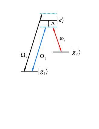
Figure 2: (Color online) The coupled system of the two-mode polaritons and a three-level atom. $\Omega_{1}$ and $\Omega_{2}$ are, respectively, the frequencies of the $c_{1}$ and $c_{2}$ modes. $\omega_{c}$ is the frequency of the classical control field and its detuning with the transition frequency $\omega_{eg_{2}}$ is $\Delta$.

We first assume that the classical field and one of two polariton modes, say $c_{1}$, satisfy the two-photon resonance condition, i.e. $\Omega_{1}=\omega_{c}+\omega_{eg_{1}}-\omega_{eg_{2}}$. In the interaction picture and taking the rotating wave approximation, the Hamiltonian Eq. (6) becomes (using $\hbar=1$)

$$h_{I} = \widetilde{\Omega}_{2}\,c_{2}^{{\dagger}}c_{2}+\Delta\left|e\right\rangle\left\langle e\right|+\xi\left|e\right\rangle\left\langle g_{2}\right|$$

$$+\left(\xi\left|e\right\rangle\left\langle g_{2}\right|+g\left(u_{1}c_{1}+u_{2}c_{2}\right)\left|e\right\rangle\left\langle g_{1}\right|+h.c\right),$$

where $\widetilde{\Omega}_{2}=\Omega_{2}-\omega_{c}-\left(\omega_{eg_{1}}-\omega_{eg_{2}}\right)$, and $\Delta=\omega_{eg_{1}}-\Omega_{1}=\omega_{eg_{2}}-\omega_{c}$. We note that $h_{I}$ possesses an invariant subspace spanned by the states $\left|e,n_{1},n_{2}\right\rangle$, $\left|g_{2},n_{1},n_{2}\right\rangle$, $\left|g_{1},n_{1}+1,n_{2}\right\rangle$ and $\left|g_{1},n_{1},n_{2}+1\right\rangle$, here $n_{1}$ and $n_{2}$ are the number of polaritons for modes $c_{1}$ and $c_{2}$, respectively. The matrix representation of the $h_{I}$ in this invariant subspace is then

$$h_{I} =\left(n_{1}\widetilde{\Omega}_{1}+n_{2}\widetilde{\Omega}_{2}\right)I$$

$$+\left(\begin{array}[]{cccc}\Delta&\xi&gu_{1}\sqrt{n_{1}+1}&gu_{2}\sqrt{n_{2}+1}\\ \xi&0&0&0\\ gu_{1}\sqrt{n_{1}+1}&0&0&0\\ gu_{2}\sqrt{n_{2}+1}&0&0&\widetilde{\Omega}_{2}\end{array}\right),$$ (12)

with $I$ being the identity matrix. Here $h_{I}$ has a zero eigenvalue corresponding to the eigenstate

$$\left|\psi_{0}\right\rangle=\cos\theta\left|g_{1},n_{1}+1,n_{2}\right\rangle-\sin\theta\left|g_{2},n_{1},n_{2}\right\rangle,$$ (14)

where $\theta$ is determined by $\tan\theta=\xi/\left(gu_{1}\sqrt{n_{1}+1}\right)$. We immediately notice that $|\psi_{0}\rangle$ is a dark state formed by polaritons and the two lower atomic levels, in contrast with that formed directly by photons. Furthermore, $|\psi_{0}\rangle$ can be factorized as

$$|\psi_{0}\rangle = |\phi_{0}\rangle\otimes|n_{2}\rangle$$ (15)

$$= \big{(}\cos\theta\left|g_{1},n_{1}+1\right\rangle-\sin\theta\left|g_{2},n_{1}\right\rangle\big{)}\otimes|n_{2}\rangle,$$

where $|\phi_{0}\rangle$ superposes different polariton number states. Considering now the $n_{1}=0$ subspace, if we manipulate the Rabi-frequency $\xi$ of the classical field adiabatically, such that $\theta$ varies from $0$ to $\pi/2$, the information of a single polarition state is then stored into the atomic state.

IV Collective Atomic Excitation dressed by polaritons

As the adiabatic manipulation described in the previous section is only accompanied by a single polariton transfer, it cannot be used to transfer or store a general state which is a superposition of multiple polariton number states. To fulfill this purpose, an ensemble of atoms is needed to serve as the quantum data bus or quantum memory. We, therefore, consider in this section $M$ identical three-level $\Lambda$-type atoms interacting with the polariton modes. Same as the single three-level atom case, we assume that only the $c_{1}$ mode satisfies the two-photon resonance condition. The Hamiltonian of the system, in the interaction picture, is (using $\hbar=1$)

$$H_{I} = \widetilde{\Omega}_{2}\,c_{2}^{{\dagger}}\,c_{2}+\Delta\sum_{j=1}^{M}\sigma_{ee}^{\left(j\right)}+\xi\sum_{j=1}^{M}\sigma_{eg_{2}}^{\left(j\right)}$$ (16)

$$+g\left[\left(u_{1}c_{1}+u_{2}c_{2}\right)\sum_{j=1}^{M}\sigma_{eg_{1}}^{\left(j\right)}+\mathrm{h.c.}\right],$$

where $\sigma_{\mu\nu}^{\left(j\right)}=\left|\mu\right\rangle_{j}\left\langle\nu\right|$ ($\mu,\nu=e,\,g_{1},\,g_{2}$) is a flip operator of the $j$th atom. To further simplify the notation, we define collective quasi-spin operators Sun

$$S = \sum_{j=1}^{M}\sigma_{ee}^{\left(j\right)},\quad T_{+}=\sum_{j=1}^{M}\sigma_{eg_{2}}^{\left(j\right)},$$

$$\text{\ }A^{{\dagger}} = \frac{1}{\sqrt{M}}\sum_{j=1}^{M}\sigma_{eg_{1}}^{\left(j\right)},$$ (17)

where $A^{\dagger}$ ($A$) characterizes the collective atomic excitations. We note that, in the large $M$ limit with low atomic excitations, the operators $A^{{\dagger}}$ and $A$ satisfy the bosonic commutation relation $\left[A,\,A^{{\dagger}}\right]=1$. The Hamiltonian Eq. (16) can now be rewritten as

$$H_{I} = \widetilde{\Omega}_{2}\,c_{2}^{{\dagger}}\,c_{2}+\Delta S$$

$$+\left(\xi\,T_{+}+g\,u_{1}\sqrt{M}\,c_{1}A^{{\dagger}}+g\,u_{2}\sqrt{M}c_{2}\,A^{{\dagger}}+\mathrm{h.c.}\right).$$

Following the procedure developed in Ref. Sun , we introduce another atomic collective excitation operator

$$C=\frac{1}{\sqrt{M}}\sum_{j=1}^{M}\sigma_{g_{1}g_{2}}^{\left(j\right)}.$$ (19)

In the large-$M$ and low excitation limit, the collective operators defined in Eqs. (17) and (19) satisfy following basic commutation relations,

$$\left[A,\,\,\,\,S\right] =A,\,\,\,\left[C,\,S\right]=0,\,\left[A,\,A^{{\dagger}}\right]=1,$$

$$\left[C,\,\,\,C^{{\dagger}}\right] =1,\,\,\,\left[T_{+},\,C^{{\dagger}}\right]=A^{{\dagger}},$$ (20)

$$\left[T_{-},\,A^{{\dagger}}\right] =C^{{\dagger}},\,\,\left[S,\,\,T_{\pm}\right]=\pm T_{\pm}.$$

The effective Hamiltonian Eq. (IV) is a function of the operators $A$, $A^{{\dagger}}$, $C$, $C^{{\dagger}}$, and $T_{\pm}$ that generate a close algebra $\mathcal{L}$, corresponding to a non-compact group $U\left(\mathcal{L}\right)$. This means that the composite system, consisting of photon, medium, and $\Lambda$-type atoms, possesses a dynamic symmetry of $U\left(\mathcal{L}\right)$. Using the symmetry analysis Sun , we construct a dark-state operator of the polariton operator $c_{1}$ and atomic operator $C$

$$D=c_{1}\cos\theta-C\sin\theta,$$

which satisfies $\left[H_{I},\,D\right]=0$ and $\left[D,\,D^{{\dagger}}\right]=1$. Furthermore, we introduce the state

$$\left|\mathbf{0}\right\rangle=\left|v\right\rangle\otimes\left|0\right\rangle_{c_{1}}\otimes\left|0\right\rangle_{c_{2}},$$

where $\left|v\right\rangle=\left|g_{1},\,g_{1},\,\cdots,\,g_{1}\right\rangle$ is the collective ground state with all atoms in their ground states, $\left|0\right\rangle_{c_{1}}$ and $\left|0\right\rangle_{c_{2}}$ are the vacuum of the polariton modes. We note that $\left|\mathbf{0}\right\rangle$ is an eigenstate of $H_{I}$ with zero eigenvalue, and consequently, a degenerate class of $H_{I}$ with zero eigenvalue can be constructed as follows

$$\left|D_{n}\right\rangle=\frac{1}{\sqrt{n!}}D^{{\dagger}n}\left|\mathbf{0}\right\rangle,$$

which can be used as a quantum memory. There also exist other eigenstates with zero eigenvalue; however, as shown in Appendix A, the adiabatic evolution does not mix them with the dark state $|D_{n}\rangle$.

V Quantum adiabatic manipulations in the presence of material media

In earlier work Lukin1 ; Lukin2 ; Lukin3 ; Sun , the EIT system was proposed as an efficient quantum memory by adiabatic quantum manipulation. In the presence of the medium, we explore the possibility of implementing such quantum manipulation by taking into account the coupling between the quantum light field and the medium.

The goal of the EIT-based quantum memory is to transmit the information of the quantum light to the low excitation state of the $\Lambda$-type atomic ensemble. To see the key point of our studies here, we would like to recall the basic physical process of the EIT-based quantum storage. If there is no interaction between the quantum light and the medium ($G=0$), the state used for quantum storage can be expressed as

$$\left|\Psi\left(\theta\right)\right\rangle=\sum_{n}c_{n}\left|d_{n}\left(\theta\right)\right\rangle\otimes\left|0\right\rangle_{B},$$

where $\left|0\right\rangle_{B}$ is the vacuum state of the collective excitation of the medium atoms and

$$\left|d_{n}\left(\theta\right)\right\rangle=(a^{\dagger}\cos\theta-C^{\dagger}\sin\theta)^{n}|0\rangle_{C}\otimes|0\rangle_{a}$$

is a dark state formed by the probe light and the collective excitations of three-level atoms. Here, $|0\rangle_{C}$ is the vacuum state defined by $C$ and $|0\rangle_{a}$ is the photon vacuum state. Therefore, a perfect quantum storage of photon states by an atomic ensemble can be realized by the following adiabatic evolution:

$$\left|\Psi\left(\theta=0\right)\right\rangle =\left|0\right\rangle_{C}\otimes\left(\sum_{n}c_{n}\left|n\right\rangle_{a}\right)\otimes\left|0\right\rangle_{B}$$

$$\rightarrow\left|\Psi\left(\theta=\frac{\pi}{2}\right)\right\rangle =\left(\sum_{n}(-1)^{n}c_{n}\left|n\right\rangle_{C}\right)\otimes\left|0\right\rangle_{a}\otimes\left|0\right\rangle_{B}.$$

As shown in the previous section, after we turn on the coupling between the medium and quantum light, the dark state $\left|d_{n}\left(\theta\right)\right\rangle$ is replaced by $\left|D_{n}\left(\theta\right)\right\rangle$, a dark state formed by the resonant mode $c_{1}$ of the polariton and the collective excitations of three-level atoms. In this case, an ideal quantum state transfer should realize the process

$$\left|0\right\rangle_{C}\otimes\sum_{n}c_{n}\left|n\right\rangle_{a}\otimes\left|0\right\rangle_{B}\rightarrow\sum_{n}c_{n}\left|n\right\rangle_{C}\otimes\left|0\right\rangle_{c_{1}}\otimes\left|0\right\rangle_{c_{2}}.$$

However, as we shall show below, quantum state transfer can only be partially achieved when $G\neq 0$. Without loss of generality, assuming that the photon state to be transferred is a Fock state, namely, the initial state of the system is

$$\left|\Psi\left(t=0\right)\right\rangle=\left|0\right\rangle_{C}\otimes\left|n\right\rangle_{a}\otimes\left|0\right\rangle_{B}.$$

We note that state $\left|n\right\rangle_{a}\otimes\left|0\right\rangle_{B}$ can be expanded using the Fock states of polaritons, which gives

$$\left|\Psi\left(0\right)\right\rangle = S_{n0}\left|0\right\rangle_{C}\otimes\left|n\right\rangle_{c_{1}}\otimes\left|0\right\rangle_{c_{2}}$$ (21)

$$+\sum_{i\neq n\text{ and }j\neq 0}S_{ij}\left|0\right\rangle_{C}\otimes\left|i\right\rangle_{c_{1}}\otimes\left|j\right\rangle_{c_{2}}$$

$$= S_{n0}\,|D_{n}(\theta=0)\rangle+|\psi^{\prime}(0)\rangle,$$

where $|\psi^{\prime}(0)\rangle=\sum_{i\neq n\text{ and }j\neq 0}S_{ij}\left|0\right\rangle_{C}\otimes\left|i\right\rangle_{c_{1}}\otimes\left|j\right\rangle_{c_{2}}$. The coefficients $S_{ij}$ can be obtained straightforwardly, in particular, when the coupling between light and medium atoms is weak, $S_{n0}$ is very close to unity. As the system evolves adiabatically to time $t$, the wave function becomes

$$\left|\Psi\left(t\right)\right\rangle=S_{n0}\,\left|D_{n}\left(\theta(t)\right)\right\rangle+\left|\psi^{\prime}\left(t\right)\right\rangle,$$ (22)

and at $\theta(t)=\pi/2$, we have

$$\left|D_{n}\left(\frac{\pi}{2}\right)\right\rangle=(-1)^{n}\,|n\rangle_{C}\otimes|0\rangle_{c_{1}}\otimes|0\rangle_{c_{2}}.$$

Therefore, the first term on the right hand side of Eq. (22) transfers the quanta of the photon to the collective excitation of the atomic ensemble; the second term, on the other hand, represents the leakage of the quantum memory.

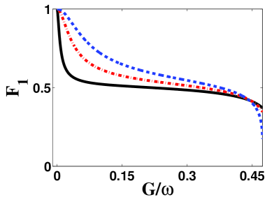
Figure 3: (Color online) The coupling strength $G$ dependence of the one-photon state transmission efficiency $F_{1}$ for $\omega_{0}=0.99\,\omega$ (black solid line), $\omega_{0}=0.95\,\omega$ (red dash-dot line), and $\omega_{0}=0.9\,\omega$ (blue dashed line).

Furthermore, to quantify the effect of the medium, we need to calculate the efficiency of the $n$-photon state transfer, i.e.,

$$F_{n}\equiv\left|S_{n0}\right|^{2}.$$

The detailed results on $F_{n}$ are presented in appendix B. In Fig. 3 we plot one-photon state transmission efficiency $F_{1}$ versus the coupling strength $G$ for different ratio of the frequencies of the quantum light and the collective excitation of the medium. We see that the presence of the medium notably reduces the transmission efficiency, especially when the quantum light is nearly resonant with the collective excitation of the medium atoms.

We notice that $F_{n}$ actually equal to 1 when $G=0$ in the resonant case and thus we can not resort to the same calculation method about the transmission efficiency shown in the appendix B. When $\omega_{0}=\omega$ together with $G=0$, there would be of singularity for the transmission efficiency if we carried out the same calculation as that in the appendix B. Physically, we can consider the cases with small detuning $\omega_{0}-\omega$ and there is not an obvious jump of the transmission efficiency as shown in Fig. 3. Actually, there is a jump of $F_{1}$ from 1 to 0.5 in the resonant case when we turn on the coupling G from $0$ to a small value. The strict resonant condition is never feasible in the practical experiment, thus we only consider two nearly resonant cases in Fig. 3.

VI Propagation of the dressed quantum light

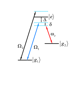
Figure 4: (Color online) Same as Fig. 2, except that here the $c_{1}$ polariton mode and the classical light field do not satisfy the two-photon resonant condition, i.e. , $\delta=\Omega_{1}-\omega_{c}-\omega_{g_{2}}\neq 0$.

To consider the dynamical process of a quantum state transfer, which is usually described by the slowing and the stopping of light, we study the dispersion and absorption properties of the dressed quantum light, propagating in a $\Lambda$-type atomic ensemble. To achieve our goal, we consider the case when the $c_{1}$ mode and the classical light field have a small two-photon detuning $\delta=\Omega_{1}-\omega_{c}-\omega_{g_{2}}\ll\Omega_{1}$ (see Fig. 4). The Hamiltonian in the interaction picture now becomes

$$H_{I} = \widetilde{\Omega}_{2}c_{2}^{{\dagger}}c_{2}+\Delta S+e^{i\delta t}\xi T_{+}$$

$$+gu_{1}\sqrt{N}c_{1}A^{{\dagger}}+gu_{2}\sqrt{N}c_{2}A^{{\dagger}}+h.c.~{}.$$

With the help of the basic commutation relations in Eq. (20), we can approximately write down the Heisenberg equations for the operators $A,\,C$, and $c_{2}$,

$$\dot{A} = -\Gamma_{A}\,A-i\,\Delta\,A-i\,g\,u_{1}\sqrt{N}\,c_{1}$$

$$-ie^{i\delta t}\,\xi C-i\,g\,u_{2}\,\sqrt{N}\,c_{2},$$

$$\dot{C} = -\Gamma_{C}\,C-ie^{-i\delta t}\,\xi\,A,$$ (23)

$$\dot{c}_{2} = -\Gamma_{c_{2}}\,c_{2}-i\widetilde{\Omega}_{2}\,c_{2}-i\,g\,u_{2}\,\sqrt{N}A,$$

where we have ignored quantum fluctuations since we only calculate the group velocity. In addition, we have phenomenologically introduced the damping rate $\Gamma_{c_{2}}$ of the mode $c_{2}$ and the decay rates $\Gamma_{A}$ and $\Gamma_{C}$ for, respectively, the states $\left|e\right\rangle$ and $\left|g_{2}\right\rangle$. $\Gamma_{A}$ and $\Gamma_{C}$ can be estimated as the spontaneous emission rates of the respective levels, which are proportional to the cube of the atomic transition frequencies, we therefore have $\Gamma_{A}\gg\Gamma_{C}$. The damping rate of the polariton mode is mainly due to the spontaneous emissions of the medium atoms and the leakage of the cavity. Since the former is negligible for a lossless medium, we can further assume $\Gamma_{C}\gg\Gamma_{c_{2}}$ for a high quality cavity.

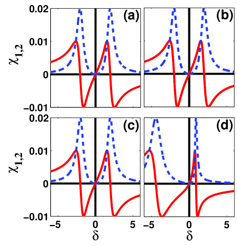
Figure 5: (Color online) $\chi_{1}$ (red solid lines) and $\chi_{2}$ (blue dashed lines) versus the two-photon detuning $\delta$ (in units of $\Gamma_{A}$, i.e., here $\Gamma_{A}=1$). (a) $\omega_{0}=0.9\,\omega$ and $G=0$; (b) $\omega_{0}=0.9\,\omega$ and $G=0.1\,\omega$; (c) $\omega_{0}=\omega$ and $G=0.1\,\omega$; (d) $\omega_{0}=\omega$ and $G=0.001\,\omega$. Other parameters are $\Gamma_{A}=1$, $\Gamma_{C}=10^{-4}$, $\Gamma_{c_{2}}=10^{-6},g\sqrt{N}=100$, and $\omega=10^{6}$.

To find a steady state solution for the above equations of motion, it is convenient to remove the fast-oscillating factors, by making the transformation $C=e^{-i\delta t}C^{\prime}$, which yields

$$\dot{A} = -\Gamma_{A}\,A-i\,\Delta\,A-i\,g\,u_{1}\sqrt{N}c_{1}$$

$$-i\xi C^{\prime}-igu_{2}\sqrt{N}\,c_{2},$$

$$\dot{C}^{\prime} = -\Gamma_{C}\,C^{\prime}-i\xi A+i\,\delta\,C^{\prime},$$ (24)

$$\dot{c}_{2} = -\Gamma_{c_{2}}\,c_{2}-i\widetilde{\Omega}_{2}\,c_{2}-i\,g\,u_{2}\sqrt{N}A.$$

The steady state solution can be obtained by letting $\dot{A}=\dot{C}^{\prime}=\dot{c}_{2}=0$, from which we find the mean value of $A$ as

$$\left\langle A\right\rangle=\frac{-igu_{1}\alpha\beta\left\langle c_{1}\right\rangle}{\alpha\beta\left(\Gamma_{A}+i\Delta\right)+\beta\xi^{2}+\alpha g^{2}u_{2}^{2}N}$$ (25)

with $\alpha=\Gamma_{C}-i\delta$ and $\beta=\Gamma_{c_{2}}+i\widetilde{\Omega}_{2}$.

It is noted here that the dressed quantum light or the propagating polaritons nearly on resonance with the $\Lambda$-type atom can be described by

$$E\left(t\right) =\varepsilon e^{-i\Omega_{1}t}+h.c.$$

$$=u_{1}\sqrt{\frac{\omega}{2V\epsilon_{0}}}c_{1}e^{-i\Omega_{1}t}+h.c.,$$

where $\epsilon_{0}$ is the permittivity of free space and $V$ is the effective mode volume, which, for simplicity, is chosen to be equal to the interaction volume. In this case, the time-independent part of the polariton field strength is $u_{1}\sqrt{\omega/2V\epsilon_{0}}.$ We remark here that the Hopfield polariton field can be understood as a displacement field or macroscopic electromagnetic field corresponding to the polarization

$$\left\langle P\right\rangle=\left\langle p\right\rangle e^{-i\Omega_{1}t}+\mathrm{h.c.}\,=\,\epsilon_{0}\,\chi\left\langle\varepsilon\right\rangle e^{-i\Omega_{1}t}+\mathrm{h.c.}\,,$$ (26)

where $\chi$ is the susceptibility. After neglecting the effect of the non-resonance polariton, the average polarization

$$\left\langle p\right\rangle=\frac{\mu}{V}\left\langle\sum_{j=1}^{N}\sigma_{eg_{2}}^{\left(j\right)}\right\rangle=\frac{\mu\sqrt{N}}{V}\left\langle A\right\rangle$$ (27)

can also be expressed in terms of the average of the exciton operator $A.$ Combining the Eqs. (25-27), we obtain

$$\chi=\frac{i2g^{2}N\alpha\beta}{\omega\left[\alpha\,\beta\left(\Gamma_{A}+i\Delta\right)+\beta\,\xi^{2}+\alpha\,g^{2}u_{2}^{2}N\right]}.$$ (28)

The real and imaginary parts $\chi_{1}$ and $\chi_{2}$ of the complex susceptibility $\chi=\chi_{1}+i\chi_{2}$ can be explicitly expressed as

$$\chi_{1} =\frac{\left(\delta\Gamma_{c_{2}}-\Gamma_{C}\widetilde{\Omega}_{2}\right)\Theta+\left(\Gamma_{C}\Gamma_{c_{2}}+\widetilde{\Omega}_{2}\delta\right)\Xi}{\Theta^{2}+\Xi^{2}}F,$$

$$\chi_{2} =\frac{\left(\Gamma_{C}\Gamma_{c_{2}}+\widetilde{\Omega}_{2}\delta\right)\Theta-\left(\delta\Gamma_{c_{2}}-\Gamma_{C}\widetilde{\Omega}_{2}\right)\Xi}{\Theta^{2}+\Xi^{2}}F,$$

where $F=2g^{2}N/\omega$, and

$$\Theta = \Gamma_{C}\left(\Gamma_{A}\Gamma_{c_{2}}-\Delta\widetilde{\Omega}_{2}\right)+\xi^{2}\Gamma_{c_{2}}$$

$$+\delta\left(\Delta\Gamma_{c_{2}}+\widetilde{\Omega}_{2}\Gamma_{A}\right)+g^{2}u_{2}^{2}N\Gamma_{C},$$

$$\Xi = -\delta\left(\Gamma_{A}\Gamma_{c_{2}}-\Delta\widetilde{\Omega}_{2}\right)+\widetilde{\Omega}_{2}\xi^{2}$$

$$+\Gamma_{C}\left(\Delta\Gamma_{c_{2}}+\widetilde{\Omega}_{2}\Gamma_{A}\right)-\delta g^{2}u_{2}^{2}N.$$

It is well known that $\chi_{1}$ and $\chi_{2}$ are related to the dispersion and absorption, respectively. In Fig. 5, $\chi_{1}$ and $\chi_{2}$ are plotted versus the two-photon detuning $\delta$.

Figure. 5(a) shows the case (i) where there is no coupling between the quantum light and the medium. The result is obviously the same as that of the conventional EIT effects. Figure. 5(b) and Fig. 5(c) demonstrate almost the same dispersion and absorption properties as that in the case without the influence of medium shown in Fig. 5(a). Figure 5(b) describes the case (ii) that the frequency of the quantum light $\omega$ and the collective excitation frequency of the medium $\omega_{0}$ is largely detuned in comparison with the parameters $g^{2}u_{2}^{2}N,\delta$ and $\Delta$, i.e.,

$$\left|\omega-\omega_{0}\right|\gg\delta,\,\Delta,\,g^{2}u_{2}^{2}N.$$

Figure. 5(c) describes the case (iii) that the coupling strength $G$ between the quantum light medium is larger than the parameters $g^{2}u_{2}^{2}N,\,\delta$ and $\Delta$, i.e., $G\,\gg\,\delta,\,\Delta,\,g^{2}u_{2}^{2}N$.

The above phenomenon, predicted by our numerical calculations, can be well explained. In the configuration, illustrated in Fig. 4, when the mode $c_{1}$ of the polariton is nearly resonant with respect to the transition between $\left|e\right\rangle$ and $\left|g_{1}\right\rangle$, the role of the mode $c_{2}$ can be neglected if this mode is off-resonace with respect to the transitions from $|e\rangle$ to $|g_{1}\rangle$ and $|g_{2}\rangle$. Then the system will be reduced to the conventional EIT model, where the mode $c_{1}$ of the polariton plays the same role as that of the quantum light, taken as the probe field. This case must lead to the same result as the conventional EIT case about the dispersion and absorption even in the presence of the medium. Now we can show that both cases (ii) and (iii) can give rise to the condition that the frequencies of the mode $c_{1}$ and $c_{2}$, i.e. $\Omega_{1}$ and $\Omega_{2}$, are largely detuned as mentioned above. We note that

$$\left|\Omega_{2}-\Omega_{1}\right|=\left(\Omega_{2}+\Omega_{1}\right)^{-1}\sqrt{\left(\omega_{0}^{2}-\omega^{2}\right)^{2}+16\omega\omega_{0}G^{2}}.$$

In the case (ii) with $\left|\omega-\omega_{0}\right|\gg\delta,\,\Delta,\,g^{2}u_{2}^{2}N$, combining the condition

$$\sqrt{\left(\omega_{0}^{2}-\omega^{2}\right)^{2}+16\omega\omega_{0}G^{2}}>\left|\omega_{0}^{2}-\omega^{2}\right|$$

with the condition $\Omega_{2}+\Omega_{1}$ being of the order of $\omega+\omega_{0}$, we can find that $\left|\Omega_{2}-\Omega_{1}\right|$ is in the order of $\left|\omega-\omega_{0}\right|$. This implies that $\left|\Omega_{2}-\Omega_{1}\right|\gg\delta,\,\Delta,\,g^{2}u_{2}^{2}N$; which shows that the large-detuning condition is satisfied. The same analysis can also be applied to the case (iii) if we note the condition

$$\sqrt{\left(\omega_{0}^{2}-\omega^{2}\right)^{2}+16\omega\,\omega_{0}\,G^{2}}>4\sqrt{\omega\omega_{0}}G.$$

Due to $|\widetilde{\Omega}_{2}|\approx\left|\Omega_{2}-\Omega_{1}\right|$, if

$$\left|\Omega_{2}-\Omega_{1}\right|\gg\delta,\,\Delta,\,g^{2}u_{2}^{2}N,$$

we can neglect all the terms, which do not have a factor of $\widetilde{\Omega}_{2}$ in the denominator and numerator of Eq. (28). After calculations, we can obtain the same expression of the susceptibility as that in the conventional EIT case Li .

For the result illustrated in Fig. 5(d), where the parameters are assumed to satisfy the condition $\left|\omega-\omega_{0}\right|/\omega\ll 1$ and $G/\omega\ll 1$, we can obtain the results, about the dispersion and the absorption, which are different from those in the conventional EIT. The phenomenon is the deformed transparent window which is assisted by the collective excitation of the medium. Indeed, if $\left|\omega-\omega_{0}\right|/\omega\ll 1$ and $G/\omega\ll 1,$ $|\widetilde{\Omega}_{2}|\approx\left|\Omega_{2}-\Omega_{1}\right|$ is smaller than or of the same order of $\delta$ and $\Delta.$ So the term related to the mode $c_{2}$ of the polariton, i.e. , $g^{2}u_{2}^{2}N\left(\Gamma_{C}-i\delta\right)$, has a dominant effect on the susceptibility $\chi.$

VII Conclusions

In conclusion, we have studied the influence of a lossless medium on an EIT system. We find that even in the presence of the medium, the whole system still has dark states. This implies that, in some cases, the EIT system in the medium can still serve as a quantum memory. We also calculate the dispersion and absorption properties of the dressed quantum light. We find that the result obtained here is quite different from that of the conventional EIT. If the coupling strength between the quantum light and the medium is sufficiently strong, the ensemble of the three-level atoms with $\Lambda$-type transitions can easily become transparent, if the usual EIT approach is applied.

VIII Acknowledgments

CPS is supported by the NSFC with grant No. 90203018, 10474104 and 60433050, and NFRPC with No. 2001CB309310 and 2005CB724508. SY is supported by NSFC No. 10674141. FN was supported in part by the National Security Agency (NSA), Laboratory of Physical Sciences (LPS), and Army Research Office (ARO); and by the National Science Foundation grant No. EIA-0130383.

Appendix A Dynamic symmetry analysis of the system

Starting from the dark state $\left|D_{n}\right\rangle$, we can use the spectrum–generating algebra method algebra to build other eigenstates of the whole system. We now introduce the bright-state polariton operator

$$B=c_{1}\sin\theta+C\cos\theta,$$

which satisfies

$$\left[B,B^{{\dagger}}\right]=1,\,\left[B,D^{{\dagger}}\right]=0,\,\left[B,D\right]=0.$$

It is straightforward to obtain the commutation relations

$$\left[H_{I},B^{{\dagger}}\right] =\varepsilon B^{{\dagger}},$$

$$\left[H_{I},A^{{\dagger}}\right] =\Delta A^{{\dagger}}+\varepsilon B^{{\dagger}}+gu_{2}\sqrt{N}c_{2}^{{\dagger}},$$

$$\left[H_{I},c_{2}^{{\dagger}}\right] =\widetilde{\Omega}_{2}c_{2}^{{\dagger}}+gu_{2}\sqrt{N}A^{{\dagger}},$$

with $\varepsilon=\sqrt{g^{2}u_{1}^{2}N\xi^{2}}$. We can introduce three independent bosonic operators

$$Q_{i}=\eta_{1}^{i}A+\eta_{2}^{i}B+\eta_{3}^{i}C,\,i=1,\,2,\,3,$$

which satisfy

$$\left[Q_{i},Q_{j}^{{\dagger}}\right]=\delta_{ij},\,\left[Q_{i},Q_{j}\right]=0$$

to diagonalize the Hamiltonian $H_{I}$, i.e.

$$\left[Q_{i},H_{I}\right]=\epsilon_{i}Q_{i}.$$

Based on the above commutation relations, we can construct eigenstates

$$\left|e\left(m_{1},m_{2},m_{3},n\right)\right\rangle=\frac{Q_{1}^{{\dagger}m_{1}}Q_{2}^{{\dagger}m_{2}}Q_{3}^{{\dagger}m_{3}}}{\sqrt{m_{1}!m_{2}!m_{3}!}}\left|D_{n}\right\rangle,$$

of the whole system, corresponding to eigenvalues

$$E\equiv E\left(m_{1},m_{2},m_{3}\right)=m_{1}\epsilon_{1}+m_{2}\epsilon_{2}+m_{3}\epsilon_{3},$$

with $m_{1},\,m_{2},\,m_{3}=0,\,1,\,2,\cdots$. The above equations show that there exists a larger class of states

$$\mathbf{S}:\left\{\left|e\left(\{m_{i}\},n\right)\right\rangle\equiv\left|D\left(\{m_{i}\},n\right)\right\rangle|n=0,\,1,\,\cdots;E=0\right\}$$

with zero eigenvalue $E\equiv E\left(m_{1},m_{2},m_{3}\right)=0$, here, $\{m_{i}\}\equiv m_{1},m_{2},m_{3}$. But we can show bellow that these states with zero eigenvalue do not mix with each other under adiabatic manipulation. Any state

$$\left|\phi\left(t\right)\right\rangle=\sum_{m_{1}m_{2}m_{3}n}c_{m_{1}m_{2}m_{3}n}\left|D\left(m_{1},m_{2},m_{3},n\right)\right\rangle,$$

with zero eigenvalue evolves according to

$$i\frac{d}{dt}c_{m_{1}m_{2}m_{3}n}\left(t\right)=\sum_{m_{1}^{\prime}m_{2}^{\prime}m_{3}^{\prime}n^{\prime}}D_{m_{1}m_{2}m_{3}n}^{m_{1}^{\prime}m_{2}^{\prime}m_{3}^{\prime}n^{\prime}}c_{m_{1}^{{}^{\prime}}m_{2}^{{}^{\prime}}m_{3}^{{}^{\prime}}n^{{}^{\prime}}}+F,$$

where $F$ is a certain functional of the eigenstates with non-zero eigenvalues, which can be neglected under the adiabatic conditions Sun-prd ; Zee , and

$$iD_{m_{1}m_{2}m_{3}n}^{m_{1}^{\prime}m_{2}^{\prime}m_{3}^{\prime}n^{\prime}}=\left\langle D\left(m_{1}^{\prime},m_{2}^{\prime},m_{3}^{\prime},n\right)\left|\partial_{t}\right|D\left(m_{1},m_{2},m_{3},n\right)\right\rangle.$$

We note that $\partial_{\theta}B=D$ and $\partial_{\theta}D=B$, and we have

$$\partial_{t}\left|D\left(m,n\right)\right\rangle=\dot{\theta}\partial_{\theta}\left|D\left(m_{1},m_{2},m_{3},n\right)\right\rangle,$$

where $\partial_{\theta}\left|D\left(m_{1},m_{2},m_{3},n\right)\right\rangle$ includes six terms: $\left|e\left(m_{1}\mp 1,m_{2},m_{3},n\pm 1\right)\right\rangle,\left|e\left(m_{1},m_{2}\mp 1,m_{3},n\pm 1\right)\right\rangle$ and $\left|e\left(m_{1},m_{2},m_{3}\mp 1,n\pm 1\right)\right\rangle$ which are all eigenstates with non-zero eigenvalues. This implies the exact result

$$\left\langle D\left(m_{1}^{\prime},m_{2}^{\prime},m_{3}^{\prime},n\right)\left|\partial_{t}\right|D\left(m_{1},m_{2},m_{3},n\right)\right\rangle=0,$$

showing that there is no mixing among the states with zero eigenvalue during the adiabatic evolution.

Appendix B Calculation of the transmission efficiency

Starting from the Hamiltonian (3), we now calculate the transmission efficiency in the coordinate representation. We recall the relation between the operators $a^{{\dagger}},\,a,\,B^{{\dagger}},\,B$ and the corresponding coordinate operators and moment operators $x_{1},\,x_{2},\,p_{1},\,$and $p_{2},$ i.e.

$$x_{1} =\sqrt{\frac{\hbar}{2m\omega}}\left(a^{{\dagger}}+a\right)\text{,}$$ (29)

$$\text{ }p_{1} =i\sqrt{\frac{m\hbar\omega}{2}}\left(a^{{\dagger}}-a\right),$$ (30)

$$x_{2} =\sqrt{\frac{\hbar}{2m\omega}}\left(B^{{\dagger}}+B\right)\text{, }$$ (31)

$$p_{2} =i\sqrt{\frac{m\hbar\omega}{2}}\left(B^{{\dagger}}-B\right),$$ (32)

where $m$ is the mass of the oscillator. We have here assumed the mass of the two oscillators to be the same. Therefore, we have the Hamiltonian

$$H_{\text{L-M}}=\frac{1}{2m}\left(p_{1}^{2}+p_{2}^{2}\right)+\frac{1}{2}\left(Ax_{1}^{2}+Bx_{2}^{2}+Cx_{1}x_{2}\right)$$ (33)

for two coupled harmonic oscillators. Here, we have neglect the zero point energy, and

$$A=m\omega^{2}\text{, }B=m\omega_{0}^{2}\text{, }C=4Gm\sqrt{\omega\omega_{0}}\,\text{. }$$ (34)

Let $\omega\neq\omega_{0}$ and define the canonical coordinates

$$\left(\begin{array}[]{c}y_{1}\\ y_{2}\end{array}\right)=\left(\begin{array}[]{cc}\cos\frac{\alpha}{2}&-\sin\frac{\alpha}{2}\\ \sin\frac{\alpha}{2}&\cos\frac{\alpha}{2}\end{array}\right)\left(\begin{array}[]{c}x_{1}\\ x_{2}\end{array}\right),$$ (35)

where

$$\tan\alpha=\frac{C}{B-A}.$$ (36)

Then we diagonalize $\ H_{\text{L-M}}$ with two decoupled harmonic oscillators

$$H_{\text{L-M}}=\frac{1}{2m}\left(p_{y_{1}}^{2}+p_{y_{2}}^{2}\right)+\frac{1}{2}\left(K_{1}y_{1}^{2}+K_{2}y_{2}^{2}\right)$$ (37)

with

$$K_{1} =\frac{A+B-K}{2},$$

$$K_{2} =\frac{A+B+K}{2},$$ (38)

and

$$K=\left(B-A\right)\sqrt{1+\frac{C^{2}}{\left(B-A\right)^{2}}}\,.$$ (39)

Therefore, the eigenenergy of the above system is

$$E=\hbar\Omega_{1}\left(n_{1}+\frac{1}{2}\right)+\hbar\Omega_{2}\left(n_{2}+\frac{1}{2}\right),$$ (40)

for $\,n_{1},\,\,n_{2}=0,\,1,\,2,\cdots,\,$and the corresponding eigenstate $\left|n_{1}\right\rangle_{c_{1}}\otimes\left|n_{2}\right\rangle_{c_{2}}$ is expressed as

$$\psi_{n_{1}n_{2}}\left(y_{1},y_{2}\right) = \mathcal{N}_{n_{1}}^{\left(b_{1}\right)}\mathcal{N}_{n_{2}}^{\left(b_{2}\right)}\exp\left\{{-\frac{1}{2}b_{1}^{2}y_{1}^{2}-\frac{1}{2}b_{2}^{2}y_{2}^{2}}\right\}$$

$$\times H_{n_{1}}\left(b_{1}y_{1}\right)H_{n_{1}}\left(b_{2}y_{2}\right),$$

in terms of the $n$th–order Hermite polynomial $H_{n}\left(\xi\right)$ with

$$\mathcal{N}_{n_{1}}^{\left(b_{1}\right)} =\left[\frac{b_{1}}{\sqrt{\pi}2^{n_{1}}n_{1}!}\right]^{\frac{1}{2}},$$

$$\mathcal{N}_{n_{2}}^{\left(b_{2}\right)} =\left[\frac{b_{2}}{\sqrt{\pi}2^{n_{2}}n_{2}!}\right]^{\frac{1}{2}},$$ (41)

$$b_{1} =\left(\frac{mK_{1}}{\hbar}\right)^{1/4},$$

$$b_{2} =\left(\frac{mK_{2}}{\hbar}\right)^{1/4}.$$

When there is no coupling between the medium and the quantum light, the Hamiltonian of the medium and quantum light is

$$H_{\text{uncoupled}}=\frac{1}{2m}\left(p_{1}^{2}+p_{2}^{2}\right)+\frac{1}{2}\left(Ax_{1}^{2}+Bx_{2}^{2}\right).$$ (42)

Therefore the eigenenergies and eigenstates $\left|n_{1}\right\rangle_{a}\otimes\left|n_{2}\right\rangle_{B}$ are given by

$$E=\hbar\omega\left(n_{1}+\frac{1}{2}\right)+\hbar\omega_{0}\left(n_{2}+\frac{1}{2}\right),\,$$ (43)

and

$$\phi_{n_{1}n_{2}}\left(x_{1},x_{2}\right) = \mathcal{N}_{n_{1}}^{\left(a_{1}\right)}\mathcal{N}_{n_{2}}^{\left(a_{2}\right)}\exp\left\{-\frac{1}{2}a_{1}^{2}x_{1}^{2}-\frac{1}{2}a_{2}^{2}x_{2}^{2}\right\}$$

$$\times H_{n_{1}}\left(a_{1}x_{1}\right)H_{n_{1}}\left(a_{2}x_{2}\right)$$

respectively, for $n_{1},\,\,n_{2}=0,\,1,\,2,\cdots\,\,$and

$$\mathcal{N}_{n_{1}}^{\left(a_{1}\right)} =\left[\frac{a_{1}}{\sqrt{\pi}2^{n_{1}}n_{1}!}\right]^{\frac{1}{2}},$$

$$\mathcal{N}_{n_{2}}^{\left(a_{2}\right)} =\left[\frac{a_{2}}{\sqrt{\pi}2^{n_{2}}n_{2}!}\right]^{\frac{1}{2}},$$

$$a_{1} =\left(\frac{mA}{\hbar}\right)^{1/4},$$

$$a_{2} =\left(\frac{mB}{\hbar}\right)^{1/4}.$$

Now we can calculate the transmission efficiency of $n$-photon state

$$F_{n} = \left|S_{n0}\right|^{2}$$

$$= \left|\left.{}_{c_{2}}\left\langle 0\right|\right.\otimes\left.{}_{c_{1}}\left\langle n\right|\otimes\left\langle v\right|\right.\left|v\right\rangle\otimes\left|n\right\rangle_{a}\otimes\left|0\right\rangle_{B}\right|^{2}$$

$$= \left|\int\int\psi_{n0}\left[y_{1}\left(x_{1},x_{2}\right),y_{2}\left(x_{1},x_{2}\right)\right]\phi_{n0}\left[x_{1},x_{2}\right]dx_{1}dx_{2}\right|^{2}$$

$$= \left|\int\int\exp\left\{-\frac{1}{2}\left(a_{1}^{2}x_{1}^{2}+a_{2}^{2}x_{2}^{2}+b_{1}^{2}y_{1}^{2}+b_{2}^{2}y_{2}^{2}\right)\right\}\right.$$

$$\times H_{n}\left(a_{1}x_{1}\right)H_{0}\left(a_{2}x_{2}\right)H_{n}\left(b_{1}y_{1}\right)H_{0}\left(b_{2}y_{2}\right)$$

$$\left.\times\mathcal{N}_{n}^{\left(b_{1}\right)}\mathcal{N}_{0}^{\left(b_{2}\right)}\mathcal{N}_{n}^{\left(a_{1}\right)}\mathcal{N}_{0}^{\left(a_{2}\right)}dx_{1}dx_{2}\right|^{2}\,.$$

To explicitly calculate the integral in the above formula we can define a new pair of coordinates,

$$\left(\begin{array}[]{c}z_{1}\\ z_{2}\end{array}\right)=\left(\begin{array}[]{cc}\cos\frac{\beta}{2}&-\sin\frac{\beta}{2}\\ \sin\frac{\beta}{2}&\cos\frac{\beta}{2}\end{array}\right)\left(\begin{array}[]{c}x_{1}\\ x_{2}\end{array}\right)\text{, }$$ (45)

where

$$\tan\beta=\frac{R}{Q-P},$$

$$P =b_{1}^{2}\cos^{2}\frac{\alpha}{2}+b_{2}^{2}\sin^{2}\frac{\alpha}{2}+a_{1}^{2},$$

$$Q =b_{1}^{2}\sin^{2}\frac{\alpha}{2}+b_{2}^{2}\cos^{2}\frac{\alpha}{2}+a_{2}^{2},$$ (46)

$$R =2\left[b_{2}^{2}\cos\frac{\alpha}{2}\sin\frac{\alpha}{2}-b_{1}^{2}\cos\frac{\alpha}{2}\sin\frac{\alpha}{2}\right].$$

Therefore, the integral

$$\int\int\exp\left\{-\frac{1}{2}\left(a_{1}^{2}x_{1}^{2}+a_{2}^{2}x_{2}^{2}+b_{1}^{2}y_{1}^{2}+b_{2}^{2}y_{2}^{2}\right)\right\}$$

$$\times H_{n}\left(a_{1}x_{1}\right)H_{0}\left(a_{2}x_{2}\right)H_{n}\left(b_{1}y_{1}\right)H_{0}\left(b_{2}y_{2}\right)dx_{1}dx_{2}\,$$

is transformed to

$$\int\int\exp\left\{-\frac{1}{2}W_{1}z_{1}^{2}-\frac{1}{2}W_{2}z_{2}^{2}\right\}$$

$$\times H_{n}\left(a_{1}x_{1}\right)H_{0}\left(a_{2}x_{2}\right)H_{n}\left(b_{1}y_{1}\right)H_{0}\left(b_{2}y_{2}\right)Jdz_{1}dz_{2}$$

where

$$J=\left|\begin{array}[]{cc}\frac{\partial x_{1}}{\partial z_{1}}&\frac{\partial x_{1}}{\partial z_{2}}\\ \frac{\partial x_{2}}{\partial z_{1}}&\frac{\partial x_{2}}{\partial z_{2}}\end{array}\right|=1$$

is the Jacobi determinant and

$$W_{1} =\frac{P+Q-S}{2},$$

$$W_{2} =\frac{P+Q+S}{2},$$ (48)

where

$$S=\left(Q-P\right)\sqrt{1+\frac{R^{2}}{\left(Q-P\right)^{2}}}$$

and

$$\left(\begin{array}[]{c}x_{1}\\ x_{2}\end{array}\right)=\left(\begin{array}[]{cc}\cos\frac{\beta}{2}&\sin\frac{\beta}{2}\\ -\sin\frac{\beta}{2}&\cos\frac{\beta}{2}\end{array}\right)\left(\begin{array}[]{c}z_{1}\\ z_{2}\end{array}\right),$$

$$\left(\begin{array}[]{c}y_{1}\\ y_{2}\end{array}\right)=\left(\begin{array}[]{cc}\cos\frac{\alpha-\beta}{2}&-\sin\frac{\alpha-\beta}{2}\\ \sin\frac{\alpha-\beta}{2}&\cos\frac{\alpha-\beta}{2}\end{array}\right)\left(\begin{array}[]{c}z_{1}\\ z_{2}\end{array}\right).$$

We note that $H_{n}\left(b_{1}y_{1}\right),\,H_{0}\left(b_{2}y_{2}\right),\,H_{n}\left(a_{1}x_{1}\right),\,H_{0}\left(a_{2}x_{2}\right)$ can be expressed as a polynomial of $z_{1}\,$and$\,z_{2}$, so that the integral (LABEL:integral_z) can be calculated with the help of the following integral formula

$$\int_{-\infty}^{+\infty}t^{n}e^{-\rho t^{2}}=\frac{1}{2}\left(1+\left(-1\right)^{n}\right)\rho^{-\frac{1}{2}\left(1+n\right)}\Gamma\left[\frac{1+n}{2}\right],$$

where $n=0,\,1,\,\cdots\,,\,\rho>0,$ and $\Gamma[n]$ is the gamma function.

For the simplest case, when $n=1$, we have

$$F_{1}=\left|\frac{4}{\pi}\sqrt{\frac{a_{1}^{3}a_{2}b_{1}^{3}b_{2}}{W_{1}W_{2}}}\times\right. \left[\frac{1}{W_{1}}\cos\frac{\alpha-\beta}{2}\cos\frac{\beta}{2}\right.$$

$$\left.\left.-\frac{1}{W_{2}}\sin\frac{\alpha-\beta}{2}\sin\frac{\beta}{2}\right]\right|^{2}\,.$$ (49)

References

(1) S. Harris, Phys. Today 50(7), 36 (1997).
(2) L. Hau, S. Harris, Z. Dutton, and C. H. Behroozi, Nature
(London) 397, 594 (1999).
(3) M. M. Kash, V. A. Sautenkov, A. S. Zibrov, L. Hollberg, G. R.
Welch, M. D. Lukin, Y. Rostovtsev, E. S. Fry and M. O. Scully, Phys. Rev.
Lett. 82, 5229 (1999).
(4) M. D. Lukin, S. F. Yelin, and M. Fleischhauer, Phys. Rev.
Lett. 84, 4232 (2000).
(5) M. Fleischhauer and M. D. Lukin, Phys. Rev. Lett. 84, 5094 (2000).
(6) M. Fleischhauer and M. D. Lukin, Phys. Rev. A 65,
022314 (2002).
(7) D. Bouwmeester, A. Ekert and A. Zeilinger (Ed.) The
Physics of Quantum Information (Springer, Berlin, 2000).
(8) E. E. Mikhailov, Y. V. Rostovtsev, G. R. Welch, J. Modern
Optics 50 , 2645 (2003).
(9) I. Novikova, Y. Xiao, D. F. Phillips, R. L. Walsworth, J.
Modern Optics 52, 2381 (2005).
(10) S. M. Dutra and K. Furuya, Phys. Rev. A 55, 3832
(1997).
(11) J. J. Hopfield, Phys. Rev. 112, 1555 (1958).
(12) C. P. Sun, Y. Li, and X. F. Liu, Phys. Rev. Lett. 91,
147903 (2003).
(13) G. R. Jin, P. Zhang, Yu-xi Liu, and C. P. Sun, Phys. Rev. B
68, 134301 (2003).
(14) M. O. Scully and M. S. Zubairy, Quantum Optics (Cambridge Univ. Press, Cambridge, 1997).
(15) Y. Li and C. P. Sun, Phys. Rev. A 69, 051802(R) (2004).
(16) B. G. Wybourne, Classical Groups for Physicists
(John Wiley, NY, 1974); M. A. Shifman, Particle Physics and Field
Theory, p. 775 (World Scientific, Singapore, 1999).