Unbounded violation of tripartite Bell inequalities

Abstract

We prove that there are tripartite quantum states (constructed from random unitaries) that can lead to arbitrarily large violations of Bell inequalities for dichotomic observables. As a consequence these states can withstand an arbitrary amount of white noise before they admit a description within a local hidden variable model. This is in sharp contrast with the bipartite case, where all violations are bounded by Grothendieck’s constant. We will discuss the possibility of determining the Hilbert space dimension from the obtained violation and comment on implications for communication complexity theory. Moreover, we show that the violation obtained from generalized GHZ states is always bounded so that, in contrast to many other contexts, GHZ states do in this case not lead to extremal quantum correlations. In order to derive all these physical consequences, we will have to obtain new mathematical results in the theories of operator spaces and tensor norms. In particular, we will prove the existence of bounded but not completely bounded trilinear forms from commutative C*-algebras.

I Introduction

Bell inequalities characterize the boundary of correlations achievable within classical probability theory under the assumption that Nature is local WernerWolf . Originally, Bell Bell proposed the inequalities, which now bear his name, in order to put the intuition of Einstein, Podolski and Rosen EPR on logically firm grounds, thus proving that an apparently metaphysical dispute could be resolved experimentally. Nowadays, the verification of the violation of Bell inequalities has become experimental routine Aspect ; Rowe ; Aspel (albeit there is a remaining desire for a unified loophole-free test). On the theoretical side—in the realm of quantum information theory—they became indispensable tools for understanding entanglement Werner ; entmulti1 ; entmulti2 ; entmulti3 and its applications in cryptography Ekert ; Acin0 ; Acin01 ; Acin1 ; Acin02 and communication complexity CCP . In fact, the insight gained from the violation of Bell inequalities enables us even to consider theories beyond quantum mechanics Masanes1 ; Wernercloning and allows to replace quantum mechanics by the violation of some Bell inequality in the set of trusted assumptions for secure cryptographic protocols Acin0 ; Acin01 ; Acin02 ; Kent ; MasanesWinter .

Most of our present knowledge on Bell inequalities and their violation within quantum mechanics is based on the paradigmatic Clauser-Horne-Shimony-Holt (CHSH) inequality CHSH . It bounds the correlations obtained in a setup where two observers can measure two dichotomic observables each. In fact, it is the only non-trivial constraint on the polytope of classically reachable correlations in this case Fine . If we allow for more observables (measurement settings) per site or more sites (parties) the picture is much less complete. Whereas for two dichotomic observables per site the complete set of multipartite ‘full-correlation inequalities’ and their maximal violations within quantum mechanics is still known WW ; ZB , the case of more than two settings is, despite considerable effort moresettings1 ; moresettings3 ; moresettings2 , largely unexplored.

One reason is, naturally, that finding all possible Bell inequalities is a computationally hard task Pit1 ; Naor and that in addition the violating quantum systems become vastly more complicated as the number of sites and dimensions increases. Another reason could be the lack of appropriate mathematics to tackle the problem. Thus far, researchers have primarily used algebraic and combinatorial techniques.

In this work, following the lines already implicit in Tsirelson , we will relate tripartite Bell inequalities with two powerful theories of mathematical analysis: operator spaces, and tensor norms. We will give new mathematical results inside these theories and show how to apply them to provide a deeper insight into the understanding of Bell inequalities, by proving some new and intriguing results on their maximal quantum violation. It is interesting to note here that operator spaces have recently also led to other applications in Quantum Information Marius .

We will start by outlining the main result and some of its implications within quantum information theory. Sec. III will then recall basic notions from the theory of operator spaces and tensor norms and bridge between the language of Bell inequalities and the mathematical theories. In Sec. IV we will prove that the violation remains bounded for GHZ states. Finally, Sec. V provides the proof for the main theorem.

II Main Result and Implications

We begin by specifying the framework. For the convenience of the non-specialist reader we will give first a brief introduction to Bell Inequalities. For further information we refer the reader to WernerWolf .

Bell inequalities can be dated back to the famous critic of Quantum Mechanics due to Einstein, Podolski and Rosen EPR . This critic was made under their believe that on a fundamental level Nature was described by a local hidden variable (LHV) model, i.e., that it is classical (realistic or deterministic) and local (or non-signaling). The latter essentially means that no information can travel faster than a maximal speed (e.g. of light) which implies in particular that the probability distribution for the outcomes of some experiment made by Alice cannot depend on what other (spatially separated) physicist Bob does in his lab. Otherwise, by choosing one or the other experiment, Bob could influence instantly Alice’s results and hence transmit information at any speed. On the other hand, saying that Nature is classical or deterministic means that the randomness in the outcomes that is observed in the experiments comes from our ignorance of Nature, instead of being an intrinsic property of it (as Quantum Mechanics postulates). That is, Nature can stay in different configurations $s$ with some probability $p(s)$ ($s$ is usually called a hidden variable). But once it is in a fixed configuration $s$, then any experiment has deterministic outputs. We note that there are non-deterministic LHV models as well, but they can all be cast into deterministic models WernerWolf . Let us formalize this a bit more.

Consider correlation experiments where each of ${N}$ spatially separated observers (Alice, Bob, Charlie,…) can measure ${M}$ different observables with outcomes $\pm 1$: $\{A_{i_{1}}\}_{i_{1}=1}^{M}$ for Alice, $\{B_{i_{2}}\}_{i_{2}=1}^{M}$ for Bob and so on. By repeating the experiment several times, for each possible configuration of the observables (Alice measuring with the aparatus $A_{i_{1}}$, Bob with the aparatus $B_{i_{2}}$, …), they can obtain a good approximation of the expected value of the product of the outcomes of such configuration $\langle A_{i_{1}}B_{i_{2}}C_{i_{3}}\cdots\rangle$. If Nature is described by a LHV model, then

$$\langle A_{i_{1}}B_{i_{2}}C_{i_{3}}\cdots\rangle=\langle A_{i_{1}}B_{i_{2}}C_{i_{3}}\cdots\rangle_{p}=\sum_{s}p(s)A_{i_{1}}(s)B_{i_{2}}(s)\cdots,$$ (1)

where $A_{i_{1}}(s)=\pm 1$ is the deterministic outcome obtained by Alice if she does the experiment $A_{i_{1}}$ and Nature is in state $s$ (notice that we are including also the locality condition when assuming that $A_{i_{1}}(s)$ is independent of $i_{2},i_{3},\ldots$).

For a quantum mechanical system in a state $\rho$ we have to set

$$\langle A_{i_{1}}B_{i_{2}}C_{i_{3}}\cdots\rangle=\langle A_{i_{1}}B_{i_{2}}C_{i_{3}}\cdots\rangle_{\rho}=\operatorname{tr}(\rho A_{i_{1}}\otimes B_{i_{2}}\otimes C_{i_{3}}\cdots)$$ (2)

where $\rho$ is a density operator acting on a Hilbert space $\mathbb{C}^{d_{1}}\otimes\cdots\otimes\mathbb{C}^{d_{N}}$ and the observables satisfy $-\mathbbm{1}\leq A_{i_{1}},B_{i_{2}},C_{i_{3}},\ldots\leq\mathbbm{1}$, describing measurements within the framework of positive operator valued measures (POVMs). Note the parallelism with (1). In fact the quantum mechanical expression coincides with the classical one if the matrices $A_{i_{1}}$’s, $B_{j_{2}}$’s, …commute with each other (and therefore can be taken diagonal in some basis $|s\rangle$), and we take the state $\rho$ to be the separable state given by $\rho=\sum_{s}p(s)|s\rangle\langle s|\otimes|s\rangle\langle s|\otimes\cdots$.

How can one then know if Nature allows for a LHV description or follows Quantum Mechanics? That is, how to discriminate between (1) and (2)? The key idea of Bell Bell was to realize that this can be done by taking linear combinations of the expectation values $\langle A_{i_{1}}B_{i_{2}}C_{i_{3}}\cdots\rangle$. So, given real coefficients $T_{i_{1}i_{2},\ldots}$, if we maximize the expression

$$\left|\sum_{i_{1},\cdots,i_{N}=0}^{M-1}T_{i_{1}\cdots i_{N}}\langle A_{i_{1}}B_{i_{2}}C_{i_{3}}\cdots\rangle\right|$$ (3)

assuming (1) we get

$$\|T\|:=\sup_{a_{i_{1}},b_{i_{2}},c_{i_{3}},\ldots=\pm 1}\left|\sum_{i\in\mathbb{Z}_{M}^{N}}T_{i_{1}\cdots i_{N}}a_{i_{1}}b_{i_{2}}c_{i_{3}}\cdots\right|.$$

Therefore, if all correlations predicted by quantum mechanics could be explained in a classical and local world, one would have the following Bell inequality:

$$\left|\sum_{i_{1},i_{2},i_{3},\ldots}T_{i_{1}i_{2}i_{3}\ldots}\operatorname{tr}(\rho A_{i_{1}}\otimes B_{i_{2}}\otimes C_{i_{3}}\cdots)\right|\leq\|T\|.$$ (4)

However, Quantum Mechanics predicts examples for which we have a violation in (4). The largest possible violation of a given Bell inequality (specified by $T$) within quantum mechanics is the smallest constant $K$ for which

$$\left|\sum_{i_{1},i_{2},i_{3},\ldots}T_{i_{1}i_{2}i_{3}\ldots}\operatorname{tr}(\rho A_{i_{1}}\otimes B_{i_{2}}\otimes C_{i_{3}}\cdots)\right|\leq K\|T\|$$ (5)

holds independent of the state and the observables. For instance, for the CHSH inequality ($M=2$, $N=2$ and $T$ the Hadamard matrix) we have $K=\sqrt{2}$ irrespective of the Hilbert space dimension. More generally, if we also allow for arbitrary ${M}$ and $T$ and just fix ${N}=2$, there is (see Section III) a universal constant (called Grothendieck’s constant) $K_{G}$ that works in (5) for all Bell inequalities, states and observables. This was firstly observed by Tsirelson Tsirelson (see also Acin-groth ). As $K_{G}$ is known to lie in between $1.676..\leq K_{G}\leq 1.782..$ the maximal Bell violation in Eq.(5) is bounded for bipartite quantum systems. This bound imposes some limitations to the use of Bell inequalities, where one usually desires as large violation as possible. Below, when talking about the implications of our main result, we will illustrate why having large violations can be useful in the contexts of communication complexity, quantum cryptography or noise robustness.

Therefore, it would be very useful to know whether in the tripartite case we still have a uniform bound for the violations. The first place in which we have found this question explicitely is in the review Tsirelson of Tsirelson in 1993. Our main result will be to prove that this is not the case.

(We will in the following use $\succeq,\simeq,\preceq$ to denote $\geq,=,\leq$ up to some universal constant).

Theorem 1 (Maximal violation for tripartite Bell inequalities).

1. For every dimension $d\in\mathbb{N}$, there exist $D\in\mathbb{N}$, a pure state $|\psi\rangle$ on $\mathbb{C}^{d}\otimes\mathbb{C}^{D}\otimes\mathbb{C}^{D}$ and a Bell inequality with traceless observables such that the violation by $|\psi\rangle$ is $\succeq\sqrt{d}$.

2. The (unnormalized) state can be taken $|\psi\rangle=\sum_{1\leq i\leq d\;1\leq j,k\leq D}\langle j|U_{i}^{\dagger}|k\rangle\;|ijk\rangle$, where $U_{i}$ are random unitaries.

3. The order ${\sqrt{d}}$ is optimal in the sense that, conversely, for every state acting on $\mathbb{C}^{d}\otimes\mathbb{C}^{D}\otimes\mathbb{C}^{D}$ and every Bell inequality with not necessarily traceless observables the violation is also $\preceq\sqrt{d}$.

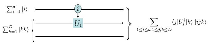
Figure 1: Quantum circuit that provides highly non-local states. Apart from using a maximally entangled state as an input, it requires the implementation of a controlled unitary with random unitaries (that is, if the control qubit is in state $|i\rangle$, the circuit applies the (random) unitary $U_{i}$)

This Theorem shows once more that random states exhibit unexpected extremal properties random1 ; random2 ; random3 ; random4 . Unfortunately, though we have a explicit form for these highly non-local states (see Figure 1), there are a couple of weaknesses in the above theorem, which mainly come from the techniques we use:

• We do not have any control on the growth of $D$ with respect to $d$.

• We do not have a explicit form for the family of inequalities for which we have unbounded violation. As it will be shown in the proof, for both the choice of the observables and the choice of the coefficients of the Bell inequality we will use a lifting argument, which in our case goes back to some application of Hahn-Banach’s theorem and the clever use of approximate unit in ideals of a $C^{*}$-algebra. This prevents us from having a constructive proof. It would be interesting to find these lifting in another way (even numerically or probabilistically).

It is important to note here (see Sec. IV) that in contrast to what is known for the ${M}=2$ case WW , GHZ states do not belong to this set of highly non-local states—they always lead to a bounded violation. Let us now discuss some of the implications of Thm.1:

Communication complexity:

Using notions from CCP0 it was shown in CCP that for every quantum state that violates a Bell inequality there is a communication complexity problem for which a protocol assisted by that state is more efficient than any classical protocol. In fact, it turns out that there is a quantitative relation between the amount of violation and the superiority of the assisted protocol.

Adapted to our case, the communication complexity problem discussed in CCP0 ; CCP ; moresettings2 is the following: Each of the three parties ($i=1,2,3$) obtains initially a random bit string encoding $(x_{i},y_{i})$, where each $y_{i}=\pm 1$ is taken from a flat distribution and $x_{i}\in\{0,\ldots,{M-1}\}$ is distributed according to $|T_{x}|/\sum_{x^{\prime}}|T_{x^{\prime}}|$ where $T_{x}=T_{x_{1},x_{2},x_{3}}$ are the coefficients appearing in the violated Bell inequality. The goal is now that every party first broadcasts a single bit and then attempts to compute the function

$$F(x,y)=\prod_{i}y_{i}T_{x}/|T_{x}|$$ (6)

upon the obtained information. The protocol was successful if all parties come to the right conclusion. If one compares the optimal classical protocol (assisted by shared randomness) with a protocol assisted by a quantum state violating the considered Bell inequality by a factor $K$, and denotes the respective probabilities of success by $P$ and $P_{K}$ then

$$\frac{P_{K}-\frac{1}{2}}{P-\frac{1}{2}}=K.$$ (7)

Let us denote by $H(P)$ the binary entropy and quantify the information $I$ about the actual value of $F(x,y)$ gained by a protocol with success probability $P$ by $I(P)=1-H(P)$. Taking the states and inequalities appearing in Thm.1 and thus setting $K\succeq\sqrt{d}$ then leads to the ratio

$$\frac{I(P_{K})}{I(P)}\succeq d\;.$$ (8)

Measuring the size of the Hilbert space:

What do measured correlations tell us about a quantum system, if we do not have a priori knowledge about the observables or even the size of the underlying Hilbert space? This type of question becomes for instance relevant in the context of cryptography where one wants to avoid any kind of auxiliary assumption necessary for security Acin0 ; Acin01 ; Acin02 ; Kent ; MasanesWinter . In the context of detecting entanglement it is easy to see that the set of entanglement witnesses that remain meaningful when disregarding the Hilbert space dimension is exactly the set of Bell inequalities. In fact, if measured correlations do not violate any Bell inequality, then they can always be produced by a separable (i.e., unentangled) state in a sufficiently large Hilbert space Acin01 . Thm.1 now shows that for multipartite systems the violation of a Bell inequality can in principle be used to estimate (lower bound) the Hilbert space dimension. It also answers a question posed by Masanes Masanes in the negative: in contrast to the case ${M}=2$ WW ; Masanes the extreme points of the set of quantum correlations observable with dichotomic measurements are in general not attained for multi-qubit systems.

Robustness against noise and detector inefficiencies:

It is well known that for ${M}=2$ the maximal quantum violation can increase exponentially in the number of sites $N$ MA ; WW . However, since the $N$ parties have to measure in coincidence, in practice with imperfect detectors, this increase comes with the handicap that also the coincidence rates then decrease exponentially. This becomes clearly different if one increases the violation without increasing $N$ as it is the case in Thm.1. So, in spite of the opaqueness of our result concerning practical implementations it does not suffer from decreasing coincidence rates.

Similarly, Thm.1 implies the existence of tripartite quantum states that can withstand an arbitrary amount of white noise before they admit a description within a local hidden variable model. To see this let $\rho$ belong to the family of states giving rise to a maximal violation $K\succeq\sqrt{d}$ and set

$$\rho^{\prime}=p\rho+(1-p)\frac{\mathbbm{1}}{\operatorname{tr}(\mathbbm{1})}.$$ (9)

As the violation $K$ is attainable for traceless observables, $\rho^{\prime}$ yields $K^{\prime}=pK$ which is still a violation whenever $p\succeq 1/\sqrt{d}$ (see Acin-groth for a similar reasoning in the bipartite case). In this context, it is a natural question to ask which is the amount of noise needed to disentangle a quantum state. It happens that this is considerably bigger. In particular, it is shown in Rungta (in a constructive way) that:

Theorem 2 (Neighborhood of the maximally mixed state).

Given $d$, there is an entangled state $\rho_{d}$ in $\mathbb{C}^{d}\otimes\mathbb{C}^{d}\otimes\mathbb{C}^{d}$ such that $\rho^{\prime}_{d}=p\rho_{d}+(1-p)\frac{\mathbbm{1}}{d^{3}}$ is still entangled whenever $p\succeq\frac{1}{d^{2}}$.

We will give an independent proof in the Appendix. Up to now the optimal value of $p$ is not known. The best bounds are given by $\frac{1}{d^{3}}\preceq p\preceq\frac{1}{d^{2}}$ Rungta ; Gurvits . It is also known that $\rho_{d}$ in Theorem 2 can be taken to be the generalized GHZ state Deuar in contrast to what we will see for the maximal violation of multipartite Bell inequalities.

III Mathematical tools

We will use tools from the theory of Operator Spaces and Tensor Norms. The use of one or the other will depend on the point of view of our problem. If we put the focus on the Bell inequalities and ask for the largest possible violation within Quantum Mechanics, then we will work with Operator Spaces and the meta-theorem we have is the following (for a precise formulation see below):

A Bell inequality for $N$ observers and $M$ dichotomic observables per site is given by a $N$-linear form $T:\ell_{\infty}^{M}\times\cdots\times\ell_{\infty}^{M}\longrightarrow\mathbb{C}$ with $\|T\|=1$. The largest possible violation within Quantum Mechanics is given by the completely bounded norm of $T$, $\|T\|_{cb}$.

If, however, we put the focus on the quantum states and ask, given a $N$-partite quantum state, which is the largest possible violation that this state gives to a Bell inequality, then we will work with the theory of Tensor Norms, and the meta-theorem now reads:

The largest possible violation that a $N$-partite $D\times\cdots\times D$ state $\rho$ gives to a Bell inequality (with an arbitrarily number of dichotomic observables) is given by the extendible tensor norm

$$\|\rho\|_{\otimes^{N}_{j=1,\alpha_{ext}}S_{1}^{D}}.$$

Operator spaces

The theory of operator spaces started with the work of Effros and Ruan in the 80’s (see e.g. EffrosRuan ; Pisierbook ) where they characterized, in an abstract sense, the structure of a subspace of a $C^{*}$-algebra. Since then, this theory has found some interesting applications in mathematical analysis. An operator space is a complex vector space $E$ and a sequence of norms $\|\cdot\|_{n}$ in the space of $E$-valued matrices $M_{n}(E)=M_{n}\otimes E$, which verify the properties

1. For all $n$, $x\in M_{n}(E)$ and $a,b\in M_{n}$ we have that $\|axb\|_{n}\leq\|a\|_{M_{n}}\|x\|_{n}\|b\|_{M_{n}}$.

2. For all $n,m$, $x\in M_{n}(E)$, $y\in M_{m}(E)$, we have that

   $$\left\|\left(\begin{array}[]{cc}x&0\\ 0&y\\ \end{array}\right)\right\|_{n+m}=\max\{\|x\|_{n},\|y\|_{m}\}$$

Any $C^{*}$-algebra has a natural operator space structure that is the resulting of embedding it inside the space $\mathcal{B}(H)$ of bounded linear operators in a Hilbert space EffrosRuan ; Pisierbook , where $M_{n}(\mathcal{B}(H))=\mathcal{B}(\ell_{2}^{n}\otimes H)$. In particular, $\ell_{\infty}^{k}$ ($=\mathbb{C}^{k}$ with the sup-norm), being a commutative $C^{*}$-algebra, has a natural operator space structure. To compute it we embed $\ell_{\infty}^{k}$ in the diagonal of $M_{k}$ (with the operator norm) and then, given $x=\sum_{i}A_{i}\otimes|i\rangle\in M_{n}(\ell_{\infty}^{k})=M_{n}\otimes\ell_{\infty}^{k}$, we have

$$\|x\|_{n}=\left\|\sum_{i}A_{i}\otimes|i\rangle\langle i|\right\|_{M_{nk}}=\max_{i}\|A_{i}\|_{M_{n}}.$$ (10)

The morphisms in the category of operator spaces (that is, the operations that preserve the structure) are called completely bounded maps. They are linear maps $u:E\longrightarrow F$ between operator spaces such that all the amplifications $u_{n}=\mathbbm{1}_{n}\otimes u:M_{n}(E)\longrightarrow M_{n}(F)$ are bounded. The cb-norm of $u$ is then defined as $\|u\|_{cb}=\sup_{n}\|u_{n}\|$. We will call $CB(E,F)$ the resulting normed space, that is, in fact, an operator space by $M_{n}(CB(E,F))=CB(E,M_{n}(F))$. Analogously one can define the cb-norm of a multilinear map $T:E_{1}\times\cdots\times E_{N}\longrightarrow F$ as $\|T\|_{cb}=\sup\|T_{n_{1},\ldots,n_{N}}\|$, where now $T_{n_{1},\ldots,n_{N}}=T\otimes\mathbbm{1}_{n_{1}}\otimes\cdots\otimes\mathbbm{1}_{n_{N}}:M_{n_{1}}(E_{1})\times\cdots\times M_{n_{N}}(E_{N})\longrightarrow M_{n_{1}\cdots n_{N}}(F)$. A multilinear map is called completely bounded if $\|T\|_{cb}<\infty$. We will denote by $CB^{N}(E_{1},\ldots,E_{N};F)$ the resulting normed space, that is also an operator space by $M_{n}(CB^{N}(E_{1},\ldots,E_{N};F))=CB^{N}(E_{1},\ldots,E_{N};M_{n}(F))$.

With these definitions, if we have a $N$-linear form $T:\ell_{\infty}^{M}\times\cdots\times\ell_{\infty}^{M}\longrightarrow\mathbb{C}$ given by $T(|i_{1}\rangle,|i_{2}\rangle,\ldots)=T_{i_{1}i_{2}\ldots}$ and we compute the usual norm and the cb-norm we obtain

$$\|T\| =\sup\{\left|\sum_{i_{1},\cdots,i_{N}=0}^{M-1}T_{i_{1}i_{2}\ldots}\epsilon^{1}_{i_{1}}\epsilon^{2}_{i_{2}}\cdots\right|\;;|\epsilon^{j}_{i_{j}}|\leq 1\},$$

$$\|T\|_{cb} =\sup\left\{\left|\sum_{i_{1},\cdots,i_{N}=0}^{M-1}T_{i_{1}i_{2}\ldots}\operatorname{tr}(\rho A_{i_{1}}\otimes B_{i_{2}}\cdots)\right|\;:\;\begin{array}[]{c}A_{i_{1}},B_{i_{2}},\ldots\in M_{D}\text{ with operator norm }\leq 1\\ \rho\in M_{D^{N}}\text{ with trace norm }\leq 1\\ \end{array}\;\right\}.$$

These expressions coincide respectively with the maximal value that one can achieve in the expression (3)

$$\left|\sum_{i_{1},\cdots,i_{N}=0}^{M-1}T_{i_{1}\cdots i_{N}}\langle A_{i_{1}}B_{i_{2}}C_{i_{3}}\cdots\rangle\right|$$

if we assume that Nature is deterministic and local, $\|T\|$, or if we assume Quantum Mechanics, $\|T\|_{cb}$. This essentially proves the meta theorem stated at the beginning of the Section. The only subtle point is that in the context of Bell inequalities everything is real while in this context of operator spaces we are in the complex case. Therefore, whenever we want to formally use this meta-theorem we will have to make some splits between real and imaginary parts.

In Grothendieck , Grothendieck proved what he called the fundamental theorem of the metric theory of tensor products. This result, known as Grothendieck’s Theorem or Grothendieck’s Inequality reads as follows:

There exists a universal constant $K_{G}$ such that no matter how we choose real coefficients $T_{ij}$ and elements $x_{i},y_{j}$ in the unit ball of a real Hilbet space $H$ with inner product $\langle\cdot,\cdot\rangle$, we have that

$$\left|\sum_{ij}T_{ij}\langle x_{i},y_{j}\rangle\right|\leq K_{G}\sup_{\epsilon_{i},\nu_{j}=\pm 1}\left|\sum_{ij}T_{ij}\epsilon_{i}\nu_{j}\right|.$$

In particular,

$$\left|\sum_{ij}T_{ij}tr(\rho A_{i}\otimes B_{j})\right|\leq K_{G}\sup_{i}\|A_{i}\|\sup_{j}\|B_{j}\|\sup_{\epsilon_{i},\nu_{j}=\pm 1}\left|\sum_{ij}T_{ij}\epsilon_{i}\nu_{j}\right|.$$ (11)

The second part tells us that Grothendieck’s Theorem provides a uniform bound $K_{G}$ for the violation of any bipartite Bell inequality with dichotomic observables. This was essentially Tsirelson’s observation Tsirelson .

But the above comments show how Grothendieck’s Theorem also implies that any bounded bilinear form from a commutative $C^{*}$-algebra has to be also completely bounded, which was firstly noticed in KumarSinclair .

Since Grothendieck stated his Theorem, a lot of effort has been devoted to find suitable multilinear generalizations (see for instance groth-mult1 ; groth-mult2 ; groth-mult3 ; groth-mult4 ; groth-mult5 ; perez-q-algebra ). However, up to know, the validity of a trilinear Grothendieck’s Theorem in the context of operator spaces (and hence in the context of Bell Inequalities) has been open. Although it is conceivable that trilinear versions of Grothendieck’s inequality hold for operator spaces, our main theorem (Theorem 1) will show that the trilinear version of (11) fails. We will rewrite this now in the language of operator spaces which is instrumental in the proof. Then we will show how this Theorem implies Theorem 1 and we will give the proof in Section V.

Theorem 3.

For every $n$, there exist $N$, a state $|\psi_{N}\rangle$, a trilinear form $T:\ell_{\infty}^{2^{n^{2}}}\times\ell_{\infty}^{2^{N^{2}}}\times\ell_{\infty}^{2^{N^{2}}}\longrightarrow\mathbb{C}$ and elements $b\in M_{n}(\ell_{\infty}^{2^{n^{2}}})$, $\hat{b}\in M_{n}(\ell_{\infty}^{2^{N^{2}}})$, with $\||\psi_{N}\rangle\|,\|T\|,\|b\|,\|\hat{b}\|\preceq 1$ and

$$\left|\langle\psi_{N}|T_{n,N,N}(b,\hat{b},\hat{b})|\psi_{N}\rangle\right|\succeq\sqrt{n}.$$

Moreover

1. The order $\sqrt{n}$ is optimal.

2. $|\psi_{N}\rangle$ can be taken $\frac{1}{\sqrt{nN}}\sum_{1\leq i\leq n\;1\leq j,k\leq N}\langle j|U_{N,i}^{\dagger}|k\rangle|ijk\rangle$ where $U_{N,i}$ are random unitaries.

Again we use $\succeq$ (resp. $\simeq$) to denote $\geq$ (resp. $=$) up to some universal constant. In particular, we obtain that

Corollary 4 (Bounded but not completely bounded trilinear forms).

Given $n$, there exists $N$ and a trilinear map $T:\ell_{\infty}^{n}\times\ell_{\infty}^{N}\times\ell_{\infty}^{N}\longrightarrow\mathbb{C}$ such that $\|T\|_{cb}\geq\|T_{n,N,N}\|\succeq\sqrt{n}\|T\|$. Moreover, the order $\sqrt{n}$ is optimal.

We will finish this section by showing how Theorem 3 implies Theorem 1. As we said before, it is simply a matter of splitting into real and imaginary parts.

Theorem 3 tells us that there exist a complex matrix $\{T_{ijk}\}_{i,j,k=1}^{N}$, $n\times n$ matrices $b_{i}$ and $N\times N$ matrices $\hat{b}_{j}$ (all of them with norm $\preceq 1$) such that

$$\left|\langle\psi_{N}|\sum_{i,j,k}T_{ijk}b_{i}\otimes\hat{b}_{j}\otimes\hat{b}_{k}|\psi_{N}\rangle\right|\succeq\sqrt{n}.$$ (12)

By splitting into real and imaginary parts it is not difficult to see that one can take in (12) $T$ real and $b_{i},\hat{b}_{j}$ hermitian. Moreover, writing $\alpha_{i}=\frac{\operatorname{tr}(b_{i})}{n}$ (so that $|\alpha_{i}|\leq 1$), $b^{1}_{i}=\alpha_{i}\mathbbm{1}_{n}$, $b^{0}_{i}=b_{i}-b^{1}_{i}$ and applying the bipartite case to show that ($\rho=|\psi_{N}\rangle\langle\psi_{N}|$)

$$\left|\sum_{i,j,k}\operatorname{tr}(\rho T_{ijk}b^{1}_{i}\otimes\hat{b}_{j}\otimes\hat{b}_{k})\right|=\left|\sum_{i,j,k}T_{ijk}\alpha_{i}\operatorname{tr}(\rho_{2,3}\hat{b}_{j}\otimes\hat{b}_{k})\right|\leq K_{G},$$

one can take the observables in (12) to be traceless.

Tensor norms

The theory of tensor norms can be traced back to the work of Murray and von Neumann in the late 30’s, but it was definitely set by Grothendieck in his seminal paper Grothendieck . Since then, several and important contributions have been made (see Defant for a modern reference).

If $X_{1},\ldots,X_{N}$ are normed spaces, by $\bigotimes_{j=1,\pi}^{N}X_{j}$ we denote the algebraic tensor product $\bigotimes_{j=1}^{N}X_{j}$ endowed with the projective norm

$$\pi(u):=\inf\left\{\sum_{i=1}^{m}\|u^{1}_{i}\|\cdots\|u^{N}_{i}\|:u=\sum_{i=1}^{m}u^{1}_{i}\otimes\cdots\otimes u^{N}_{i}\right\}.$$

This tensor norm is both commutative and associative, in the sense that $\bigotimes_{j=1,\pi}^{N}X_{j}=\bigotimes_{j=1,\pi}^{N}X_{\sigma(j)}$ for any permutation of the indices $\sigma$ and that $\bigotimes_{j=1,\pi}^{N}\left(\bigotimes_{i_{j}=1,\pi}^{N_{j}}X^{j}_{i_{j}}\right)=\bigotimes_{j=1,i_{j}=1,\pi}^{N,N_{j}}X^{j}_{i_{j}}$. The projective norm $\pi$ is in duality with the injective norm $\epsilon$, defined on $\bigotimes_{j=1}^{N}X_{j}$ as

$$\epsilon(u):=\sup\left\{\left|\sum_{i=1}^{m}\phi^{1}(u^{1}_{i})\cdots\phi^{N}(u^{N}_{i})\right|:\phi^{j}\in X_{j}^{*},\|\phi^{j}\|\leq 1\right\}\;,$$

where $X_{j}^{*}$ denotes the topological dual of $X_{j}$ and $u=\sum_{i=1}^{m}u^{1}_{i}\otimes\cdots\otimes u^{N}_{i}$. That is, if $E_{j}$ is a finite dimensional normed space for every $j=1,\cdots,N$, we have $\left(\bigotimes_{j=1,\pi}^{N}E_{j}\right)^{*}=\bigotimes_{j=1,\epsilon}^{N}E^{*}_{j}$. Moreover, the dual of the $\pi$ tensor product can also be isometrically identified with the space of $N$-linear forms (with its usual operator norm). In fact, we have the natural isometric identification,

$$\mathcal{L}^{N}(E_{1},\ldots,E_{N};\mathbb{C})=(\bigotimes_{j=1,\pi}^{N}E_{j})^{*}=\mathcal{L}(E_{1},\bigotimes_{j=2,\epsilon}^{N}E^{*}_{j}).$$ (13)

Following Defant (or Floret for the multilinear version) we define a tensor norm $\beta$ of order $N$ as a way of assigning to every $N$-tuple of normed spaces $(X_{1},\ldots,X_{N})$ a norm on $\bigotimes_{j=1}^{N}X_{j}$ (we call $\bigotimes_{j=1,\beta}^{N}X_{j}$ to the resulting normed space) such that

• $\epsilon\leq\beta\leq\pi$

• $\left\|\bigotimes_{j=1}^{N}u_{j}:\bigotimes_{j=1,\beta}^{N}X_{j}\longrightarrow\bigotimes_{j=1,\beta}^{N}Y_{j}\right\|\leq\prod_{j=1}^{N}\|u_{j}\|$, for every choice of linear bounded operators $u_{j}:X_{j}\longrightarrow Y_{j}$. This is called the metric mapping property.

Sometimes we will use the notation $\bigotimes_{\beta}(X_{1},\cdots,X_{N})$ instead of $\bigotimes_{j=1,\beta}^{N}X_{j}$ to distinguish some space.

We will say that $\beta$ is finitely generated if, for every $X_{j}$, $j=1,\cdots,N$, and $z\in\bigotimes_{j=1}^{N}X_{j}$ we have

$$\beta(z;X_{1},\cdots,X_{N})=\inf\{\beta(z;E_{1},\cdots,E_{N}):E_{j}\in FIN(X_{j}),z\in\bigotimes_{j=1}^{N}E_{j}\};$$

where we denote $FIN(X)=\{E\subset X|\dim E<\infty\}$ (and $COFIN(X)=\{E\subset X|E\text{ is closed and }\dim(X/E)<\infty\}$).

As one can find in (Defant, , Sec. 17) and (Floret, , Sec. 4) tensor norms are in one-to-one duality with ideals of multilinear operators. We explain this in which follows:

A normed (Banach) ideal of $N$-linear continuous operators between Banach spaces is a pair $(\mathcal{A},\|\cdot\|_{\mathcal{A}})$ such that

• $\mathcal{A}(X_{1},\cdots,X_{N};Y)=\mathcal{A}\cap\mathcal{L}^{N}(X_{1},\cdots,X_{N};Y)$ is a linear subspace of $\mathcal{L}^{N}(X_{1},\cdots,X_{N};Y)$ and the restriction $\|\cdot\|_{\mathcal{A}}|_{\mathcal{A}(X_{1},\cdots,X_{N};Y)}$ is a (complete) norm.

• If $u_{j}\in\mathcal{L}(Z_{j},X_{j})$, $T\in\mathcal{A}(X_{1},\cdots,X_{N};Y)$ and $v\in\mathcal{L}(Y,Z)$, then the composition $v\circ T\circ(u_{1},\cdots,u_{N})$ is in $\mathcal{A}$, and

  $$\|v\circ T\circ(u_{1},\cdots,u_{N})\|_{\mathcal{A}}\leq\|v\|\|T\|_{\mathcal{A}}\|u_{1}\|\cdots\|u_{N}\|.$$

• The operator $\mathbb{K}^{N}\ni(x_{1},\cdots,x_{N})\mapsto x_{1}\cdots x_{N}\in\mathbb{K}$ is in $\mathcal{A}$ and it has $\|\cdot\|_{\mathcal{A}}$-norm equal to one.

An ideal $(\mathcal{A},\|\cdot\|_{\mathcal{A}})$ is called maximal if $\|T\|_{\mathcal{A}^{\max}}:=\sup\{\|q_{L}^{Y}\circ T|_{E_{1}\times\cdots\times E_{N}}\|_{\mathcal{A}}|E_{j}\in FIN(X_{j}),L\in COFIN(Y)\}<\infty$ implies $T\in\mathcal{A}$ and $\|T\|_{\mathcal{A}}=\|T\|_{\mathcal{A}^{\max}}$.

The following theorem shows the duality mentioned above

Theorem 5.

Let $(\mathcal{A},\|\cdot\|_{\mathcal{A}})$ be a normed ideal of N-linear continuous mappings between Banach spaces. Then $(\mathcal{A},\|\cdot\|_{\mathcal{A}})$ is maximal if and only if there exists a finitely generated tensor norm $\beta$ of order $N+1$ such that

$$\mathcal{A}(X_{1},\cdots,X_{N};Y^{*})=(\bigotimes_{\beta}(X_{1},\cdots,X_{N},Y))^{*},$$

$$\mathcal{A}(X_{1},\cdots,X_{N};Y)=(\bigotimes_{\beta}(X_{1},\cdots,X_{N},Y^{*}))^{*}\cap\mathcal{L}^{N}(X_{1},\cdots,X_{N};Y).$$

Here both identifications are isometric.

For the purposes of this paper we will only need two of these ideals: the extendible and the $(1;2)$-summing multilinear operators.

Extendible multilinear operators

The lack of a multilinear Hahn-Banach extension theorem has motivated a considerable effort in the search of partial positive results (see Hahn-Banach1 ; Hahn-Banach2 ; Hahn-Banach3 ; Hans-paper and the references therein). In this context, the natural space to work with is the space of extendible multilinear forms. That is, those continuous multilinear forms $T:X_{1}\times\cdots\times X_{n}\longrightarrow\mathbb{C}$ (here $X_{j}$ are Banach spaces) such that for every choice of superspaces $Y_{j}\supset X_{j}$, there is a continuous and multilinear extension $\tilde{T}:Y_{1}\times\cdots\times Y_{n}\longrightarrow\mathbb{C}$. We define the extendible norm of $T$ as

$$\|T\|_{ext}=\sup_{Y_{j}}\inf_{\tilde{T}}\|\tilde{T}\|,$$

where the sup runs among all possible superspaces $Y_{j}$ and the inf among all possible extensions $\tilde{T}$. As it can be found in Hahn-Banach2 , for infinite dimensional spaces $X_{j}$, $\|T\|_{ext}$ can be in general $\infty$. We say then that $T$ is extendible if $\|T\|_{ext}<\infty$.

It can be easily seen that the extendible n-linear forms constitute a Banach ideal, which we denote by $\mathcal{L}^{n}_{ext}$. Actually, it is trivial to check that $(\bigotimes_{j=1,\alpha_{ext}}^{n}X_{j})^{*}=\mathcal{L}^{n}_{ext}(X_{1},\cdots,X_{n})$ isometrically, if we define the well known (KiRa , Sec. 3) finitely generated tensor norm

$$\alpha_{ext}(u;X_{1},\cdots,X_{n})=\inf\{\pi(u;Y_{1},\cdots,Y_{n}):X_{j}\subset Y_{j}\},$$

where the $\inf$ is taken among all superspaces $Y_{j}$ of $X_{j}$.

$\alpha_{ext}$ is called the extendible tensor norm (and it is, of course, the tensor norm associated to the ideal of extendible multilinear forms in the sense of Theorem 5).

The next lemma will be a central result to connect this mathematical theory with the context of Bell inequalities:

Lemma 6.

Let $X_{1},\cdots,X_{n}$ be $n$ Banach spaces and $u\in\bigotimes_{j=1}^{n}X_{j}$. We have

$$\alpha_{ext}(u)=\sup_{M,A^{1}_{i_{1}},\cdots,A^{n}_{i_{n}}}\left|\sum_{i_{1},\cdots,i_{n}=1}^{k}M_{i_{1}\cdots i_{n}}\langle A^{1}_{i_{1}}\otimes\cdots\otimes A^{n}_{i_{n}},u\rangle\right|,$$

where the $\sup$ is taken among $(A^{1}_{i_{1}})_{i_{1}=1}^{k}\subset B_{{X^{*}_{1}}},\cdots,(A^{n}_{i_{n}})_{i_{n}=1}^{k}\subset B_{{X^{*}_{n}}},$ $\|(M_{i_{1}\cdots i_{n}})_{i_{1},\cdots,i_{n}=1}^{k}\|_{\bigotimes_{j=1,\varepsilon}^{n}\ell_{1}^{k}}\leq 1$, $k\in\mathbb{N}$, and the brackets denote as usual the action by duality.

Proof.

By the injectivity of $\ell_{\infty}$ (see for instance (Defant, , Chap I.1)), it follows that

$$\alpha_{ext}(u)=\sup\left\{\|a_{1}\otimes\cdots\otimes a_{n}(u)\|_{\bigotimes_{j=1,\pi}^{n}\ell_{\infty}^{k}}\mid a_{j}:X_{j}\rightarrow\ell_{\infty}^{k},\|a_{j}\|\leq 1,j=1,\cdots,n;k\in\mathbb{N}\right\}.$$

Now, we know that $\mathcal{L}(X_{j},\ell_{\infty}^{k})$ is isometrically isomorphic to $\ell_{\infty}^{k}(X^{*}_{j})$ (see for instance (Defant, , Chap I.3)). Thus, given $a_{j}\in\mathcal{L}(X_{j},\ell_{\infty}^{k})=\ell_{\infty}^{k}(X^{*}_{j})$ by $a_{j}=\sum_{i_{j}=1}^{k}|i_{j}\rangle\otimes A_{i_{j}}$, we have

$$\|a_{1}\otimes\cdots\otimes a_{n}(u)\|_{\bigotimes_{j=1,\pi}^{n}\ell_{\infty}^{k}}=\|\sum_{i_{1},\cdots,i_{n}=1}^{k}\langle A^{1}_{i_{1}}\otimes\cdots\otimes A^{n}_{i_{n}},u\rangle|i_{1}\rangle\otimes\cdots\otimes|i_{n}\rangle\|_{\bigotimes_{j=1,\pi}^{n}\ell_{\infty}^{k}}=$$

$$=\sup\{|\sum_{i_{1},\cdots,i_{n}=1}^{k}\langle A^{1}_{i_{1}}\otimes\cdots\otimes A^{n}_{i_{n}},u\rangle T(|i_{1}\rangle,\cdots,|i_{n}\rangle)|:T\in B_{(\bigotimes_{j=1,\pi}^{n}\ell_{\infty}^{k})^{*}}\}.$$

The statement follows now easily. ∎

With this at hand we can now formalize the meta-theorem given at the introduction of Section III:

Theorem 7.

Given a $N$-partite $D_{1}\times\cdots\times D_{N}$ quantum state $\rho$, the largest possible violation that this state gives to a Bell inequality of an arbitrarily number of dichotomic observables is upper bounded by

$$2^{N-1}\|\rho\|_{\bigotimes_{j=1,\alpha_{ext}}^{N}S_{1}^{D_{j}}}.$$

Proof.

Given a Bell inequality with (real) coefficients $T_{i_{1},\ldots,i_{N}}$ and observables $-\mathbbm{1}\leq A_{i_{1}},B_{i_{2}},\ldots\leq\mathbbm{1}$, it is clear by the definition of $\alpha_{ext}$ that

$$\left|\sum_{i_{1},i_{2},\ldots}T_{i_{1},i_{2},\ldots}\operatorname{tr}(\rho A_{i_{1}}\otimes B_{i_{2}}\otimes\cdots)\right|\leq\|\rho\|_{\bigotimes_{j=1,\alpha_{ext}}^{N}S_{1}^{D_{j}}}\sup_{\epsilon^{j}_{i_{j}}\in\mathbb{C},|\epsilon^{j}_{i_{j}}|=1}\left|\sum_{i_{1},i_{2},\ldots}T_{i_{1},i_{2},\ldots}\epsilon^{1}_{i_{1}}\epsilon^{2}_{i_{2}}\cdots\right|.$$

To finish the proof of the Theorem it is enough to notice that (see (Gustavo, , Proposition 19))

$$\sup_{\epsilon^{j}_{i_{j}}\in\mathbb{C},|\epsilon^{j}_{i_{j}}|=1}\left|\sum_{i_{1},i_{2},\ldots}T_{i_{1},i_{2},\ldots}\epsilon^{1}_{i_{1}}\epsilon^{2}_{i_{2}}\cdots\right|\leq 2^{N-1}\sup_{\epsilon^{j}_{i_{j}}=\pm 1}\left|\sum_{i_{1},i_{2},\ldots}T_{i_{1},i_{2},\ldots}\epsilon^{1}_{i_{1}}\epsilon^{2}_{i_{2}}\cdots\right|.$$

∎

Summing operators

Since the work of Grothendieck Grothendieck , the class of absolutely summing linear operators plays a crucial role in the theory of tensor norms (see DiJaTo for a reference). Motivated by that, A. Pietsch defined in Pietsch the following class of multilinear operators:

A multilinear form $T:X_{1}\times\cdots\times X_{N}\longrightarrow\mathbb{C}$ is called $(s;r)$-summing $(1\leq s,r<\infty)$ if there exists a constant $K$ such that for any choice of finite sequences $(x^{j}_{i})_{i}\subset X_{j}$, we have that

$$\left(\sum_{i}\left|T(x^{1}_{i},\ldots,x^{N}_{i})\right|^{s}\right)^{\frac{1}{s}}\leq K\prod_{j=1}^{N}\|(x^{j}_{i})_{i}\|_{r}^{\omega},$$ (14)

where $\|(x^{j}_{i})_{i}\|_{r}^{\omega}$ denotes the supremum, among all elements $x_{j}^{*}$ in the unit ball of the dual space $X_{j}^{*}$, of

$$\left(\sum_{i}\left|x^{*}_{j}(x^{j}_{i})\right|^{r}\right)^{\frac{1}{r}}.$$

The smallest $K$ valid in equation (14) is called the $(s;r)$ norm of $T$, and we write $\|T\|_{(s;r)}$. The key result is the following generalization of Grothendieck’s inequality, which appears explicitly in (perez-q-algebra, , Corollary 2.5) (see also groth-mult1 ; groth-mult2 ; Hans-paper ; groth-mult3 ).

Theorem 8.

Every extendible $N$-linear form $T$ is $(1;2)$-summing and $\|T\|_{(1;2)}\leq K_{G}2^{\frac{N-2}{2}}\|T\|_{ext}$, where $K_{G}$ is Grothendieck’s constant.

IV Bounded violations for GHZ states

The maximal violation of multipartite Bell inequalities with two dichotomic observables per site WW ; ZB ; MA is known to be attained for GHZ states $|\psi\rangle=\frac{1}{\sqrt{n}}\sum_{i=0}^{n-1}|iii\rangle$ (where $n=2$ is sufficient in this case). In contrast to that, we will show here that GHZ states do not give rise to the maximal violation in Thm.1 but rather lead to a bounded violation. In other words, there is a fixed amount of noise (independent of the dimension) which makes the considered correlations of the GHZ state admit a description within a local hidden variable model.

Before proving that we need a bit of work. We call $\rho$ the unnormalized GHZ state $\sum_{ij}|i\rangle\langle j|\otimes|i\rangle\langle j|\otimes|i\rangle\langle j|$ as a member of $\bigotimes_{j=1}^{3}S_{1}^{n}$ ($S_{1}^{n}$ the Banach space of trace class operators on a $n$-dimensional Hilbert space $\ell_{2}^{n}$). When we consider a tensor norm $\alpha$ on $\bigotimes_{j=1}^{3}S_{1}^{n}$, $\rho^{*}$ will be the same element as $\rho$, but considered in the dual $(\bigotimes_{j=1,\alpha}^{3}S_{1}^{n})^{*}$. The key point is the following result,

Proposition 9.

For every tensor norm $\alpha$,

$$\|\rho\|_{\bigotimes_{j=1,\alpha}^{3}S_{1}^{n}}\cdot\|\rho^{*}\|_{(\bigotimes_{j=1,\alpha}^{3}S_{1}^{n})^{*}}=n^{2}.$$

We will follow (GL, , Theorem 2.5). First we will need the next

Lemma 10.

Let $\alpha$ be any tensor norm and $A=\otimes_{j=1,\alpha}^{3}S_{1}^{n}$. Let $G$ be a topological compact group such that $G\subset isom(A,A)$, the group of isometries of $A$. We suppose:

1. $g\rho=\rho$ for every $g\in G$.

2. Given $L\in A^{*}$, if $L\circ g=L$ for every $g\in G$, then $L=\lambda\rho^{*}$ for some constant $\lambda$.

Then we have that $\|\rho\|_{A}\cdot\|\rho^{*}\|_{A^{*}}=n^{2}$.

Proof.

Let us take $L\in A^{*}$ such that $\|L\|_{A^{*}}$=1 and $L(\rho)=\|\rho\|_{A}$. Let $dg$ be the Haar measure on $G$. We define $L_{0}=\int_{G}L\circ gdg$. It is easy to see that $L_{0}$ is well defined and belongs to $A^{*}$ with $\|L_{0}\|_{A^{*}}\leq\|L\|_{A^{*}}$. Now, by (i), $L_{0}(\rho)=\int_{G}L\circ g(\rho)dg=L(\rho)$.

On the other hand, for every $g^{\prime}\in G$ we have $L_{0}\circ g^{\prime}=\int_{G}L\circ g\circ g^{\prime}dg=\int_{G}L\circ gdg=L_{0}$, where we have used the translational invariance of the Haar measure. Using (ii) we conclude that $L_{0}=\lambda\rho^{*}$. We have

$$\|\rho\|_{A}=L(\rho)=L_{0}(\rho)=\lambda\rho^{*}(\rho)=\lambda n^{2}.$$

And also

$$\lambda\|\rho^{*}\|_{A^{*}}=\|\lambda\rho^{*}\|_{A^{*}}=\|L_{0}\|_{A^{*}}\leq\|L\|_{A^{*}}=1.$$

Then $\|\rho^{*}\|_{A^{*}}\leq\frac{1}{\lambda},$ and thus $\|\rho\|_{A}\cdot\|\rho^{*}\|_{A^{*}}\geq n^{2}$. The other inequality is trivial.

∎

Using the previous lemma we can easily prove Proposition 9:

Proof.

We only need to show that there exists a topological compact subgroup of $isom(A,A)$ which verifies the hypothesis of Lemma 10.

For every $\varepsilon=(\epsilon_{1},\cdots,\epsilon_{n})$, where $\epsilon_{i}=\pm 1$, we consider $g_{\varepsilon}:\mathbb{C}^{n}\longrightarrow\mathbb{C}^{n}$ such that $g_{\varepsilon}(|i\rangle)=\epsilon_{i}|i\rangle$. For every $\sigma$ permutation of $\{1,\cdots,n\}$ we consider $h_{\sigma}:\mathbb{C}^{n}\longrightarrow\mathbb{C}^{n}$ such that $h_{\sigma}(|i\rangle)=|\sigma(i)\rangle$. Now we take the group ${G}$ generated by the elements of the form

$$(g_{\varepsilon}^{*}\otimes g_{\theta})\otimes(g_{\varepsilon}^{*}\otimes g_{\theta})\otimes id\,,\;(g_{\varepsilon}^{*}\otimes g_{\theta})\otimes id\otimes(g_{\varepsilon}^{*}\otimes g_{\theta})\text{ and }(h_{\sigma}^{*}\otimes h_{\tau})\otimes(h_{\sigma}^{*}\otimes h_{\tau})\otimes(h_{\sigma}^{*}\otimes h_{\tau}).$$

It is clear that $G$ is a compact subgroup of $isom(A,A)$ and that ${G}$ verifies (i). Let us check (ii). Let

$$L=\sum_{i,j,k,l,m,n}\lambda_{i,j,k,l,m,n}|i\rangle\langle j|\otimes|k\rangle\langle l|\otimes|m\rangle\langle n|$$

be an arbitrary element of $A^{*}$. We take ${g}=(g_{\varepsilon}^{*}\otimes g_{\theta})\otimes id\otimes(g_{\varepsilon}^{*}\otimes g_{\theta})$ in ${G}$. If we have $L=L\circ{g}$, we get, for every $i,j,k,l,m,n$,

$$\lambda_{i,j,k,l,m,n}=\lambda_{i,j,k,l,m,n}\epsilon_{i}\theta_{j}\epsilon_{m}\theta_{n},$$

for every choice of signs $\epsilon_{i},\theta_{j}$. Therefore, $\lambda_{i,j,k,l,m,n}=\lambda_{i,j,k,l,m,n}\delta_{i,m}\delta_{j,n}$. Then

$$L=\sum_{i,j,k,l}\lambda_{i,j,k,l}|i\rangle\langle j|\otimes|k\rangle\langle l|\otimes|i\rangle\langle j|.$$

We can repeat the step before (taking now $g=(g_{\varepsilon}^{*}\otimes g_{\theta})\otimes(g_{\varepsilon}^{*}\otimes g_{\theta})\otimes id$ to see that, in fact,

$$L=\sum_{i,j}\lambda_{i,j}|i\rangle\langle j|\otimes|i\rangle\langle j|\otimes|i\rangle\langle j|.$$

Finally, taking $g=(h_{\sigma}^{*}\otimes h_{\tau})\otimes(h_{\sigma}^{*}\otimes h_{\tau})\otimes(h_{\sigma}^{*}\otimes h_{\tau})\in{G},$ we see that $\lambda_{i,j}=\lambda_{\sigma(i),\tau(j)}$ for every permutations $\tau,\sigma$ and every $i,j$. Then, we get that $\lambda_{i,j}=\lambda$, which finishes the proof. ∎

And finally we can get the desired bound for the GHZ violation:

Theorem 11 (GHZ bound).

Given the tripartite GHZ state $|\psi\rangle=\frac{1}{\sqrt{n}}\sum_{i=0}^{n-1}|iii\rangle$, the largest possible quantum violation for a Bell inequality with dichotomic observables is upper bounded by $4\sqrt{2}K_{G}$.

Proof.

By Theorem 7 it is enough to show that for the unnormalized GHZ state $\rho=\sum_{i,j=0}^{n-1}|i\rangle\langle j|\otimes|i\rangle\langle j|\otimes|i\rangle\langle j|$ we have $\|\rho\|_{\bigotimes_{j=1,\alpha_{ext}}^{3}S_{1}^{n}}\leq K\cdot n.$ Due to Proposition 9 we only have to prove that $\|\rho^{*}\|_{ext}\geq\frac{1}{K}n$. To see this, we use that by Thm.8 $\|T\|_{(1;2)}\leq K\|T\|_{ext},$ and then it remains to be proven that $\|\rho^{*}\|_{{\mathcal{L}}_{(1;2)}^{3}(S_{1}^{n})}\geq n$. For that we consider the sequence $(|r\rangle\langle 0|)_{r=1}^{n}\subset S_{1}^{n}$, which verifies $\|(|r\rangle\langle 0|)_{r}\|_{2}^{w}\leq 1$, and $\sum_{r}\rho^{*}(|r\rangle\langle 0|,|r\rangle\langle 0|,|r\rangle\langle 0|)=n$. ∎

Remark 12.

Note that Theorem 11 holds also for $N$ parties, where now the constant can be taken $K_{G}(2\sqrt{2})^{N-1}$. In Zukowski93 an explicit set of inequalities was derived for which GHZ states achieve a violation of the order $(\pi/2)^{N}$.

V Proof of the Main Theorem

More on operator spaces

Ruan’s Theorem Pisierbook ; EffrosRuan ; Ruan assures that any operator space can be considered as a closed subspace of $\mathcal{B}(H)$ with the inherited sequence of matrix norms. Then we can define the minimal tensor product of two operator spaces $E\subset\mathcal{B}(H)$ and $F\subset\mathcal{B}(K)$ as the operator space given by

$$E\otimes_{\min}F\subset\mathcal{B}(H\otimes K).$$

In particular, $M_{n}(E)=M_{n}\otimes_{\min}E$ for every operator space $E$. The tensor norm $\min$ in the category of operator spaces will play the role of $\epsilon$ in the classical theory of tensor norms. In particular it is injective, in the sense that if $E\subset X$ and $F\subset Y$, then $E\otimes_{\min}F\subset X\otimes_{\min}Y$ as operator spaces. The analogue of the $\pi$ tensor norm is the projective tensor norm, defined as

$$\|u\|_{M_{n}(E\otimes^{\wedge}F)}=\inf\{\|\alpha\|_{M_{n,lm}}\|x\|_{M_{l}(E)}\|y\|_{M_{m}(F)}\|\beta\|_{M_{lm,n}}:u=\alpha(x\otimes y)\beta\},$$

where $u=\alpha(x\otimes y)\beta$ means the matrix product

$$u=\sum_{rsijpq}\alpha_{r,ip}\beta_{jq,s}|r\rangle\langle s|\otimes x_{ij}\otimes y_{pq}\in M_{n}\otimes E\otimes F.$$

Both tensor norms ${\wedge}$ and $\min$ are associative and commutative and they share the duality relations of their classical counterparts $\pi$ and $\epsilon$. In fact, for finite dimensional operator spaces we have the natural completely isometric identifications

$$(E\otimes^{\wedge}F)^{*}=CB^{2}(E,F;\mathbb{C})=CB(E,F^{*})=E^{*}\otimes_{\min}F^{*},$$ (15)

where, given an operator space $E$, we define its dual operator space $E^{*}$ via the identification $M_{n}(E^{*})=CB(E,M_{n})$.

Depending on the way one embeds a Banach space inside $\mathcal{B}(H)$, the same Banach space can have a completely different operator space structure. This happens even in the simplest example: the case of a Hilbert space. A trivial way of embedding a finite dimensional Hilbert space $\ell_{2}^{n}$ inside some $\mathcal{B}(H)$ is to put it into the first column (resp. row) of $M_{n}$, that is, $|i\rangle\mapsto|i\rangle\langle 0|$ (resp. $|i\rangle\mapsto|0\rangle\langle i|$). This gives us the column operator space $C_{n}$ (resp. the row operator space $R_{n}$). It is trivial to verify

$$\left\|\sum_{i}A_{i}\otimes|i\rangle\right\|_{M_{m}\otimes_{\min}R_{n}}=\left\|\sum_{i}A_{i}A_{i}^{\dagger}\right\|^{\frac{1}{2}},\quad\quad\left\|\sum_{i}A_{i}\otimes|i\rangle\right\|_{M_{m}\otimes_{\min}C_{n}}=\left\|\sum_{i}A_{i}^{\dagger}A_{i}\right\|^{\frac{1}{2}}.$$

We can also define the intersection of these two operator spaces $\operatorname{RC}_{n}=R_{n}\cap C_{n}$, where given two operator spaces $E,F$ (Pisierbook, , page 55)

$$\|\cdot\|_{M_{n}\otimes_{\min}E\cap F}=\max\{\|\cdot\|_{M_{n}\otimes_{\min}E},\|\cdot\|_{M_{n}\otimes_{\min}F}\}.$$

We will denote by $\operatorname{RC}^{2}_{n}$ to $\operatorname{RC}_{n}\otimes_{\min}\operatorname{RC}_{n}$. We have the following concrete expressions

$$\left\|\sum_{i}A_{i}\otimes|i\rangle\right\|_{M_{m}\otimes_{\min}\operatorname{RC}_{n}}=\max\left\{\left\|\sum_{i}A_{i}A_{i}^{\dagger}\right\|^{\frac{1}{2}},\left\|\sum_{i}A_{i}^{\dagger}A_{i}\right\|^{\frac{1}{2}}\right\},$$

$$\left\|\sum_{ij}A_{ij}\otimes|ij\rangle\right\|_{M_{m}\otimes_{\min}\operatorname{RC}_{n}^{2}}= \max\left\{\left\|\sum_{i}A_{i}A_{i}^{\dagger}\right\|^{\frac{1}{2}},\left\|\sum_{i}A_{i}^{\dagger}A_{i}\right\|^{\frac{1}{2}},\right.$$ (16)

$$\left.\left\|\sum_{ij}A_{ij}\otimes|i\rangle\langle j|\right\|_{M_{m}\otimes_{\min}M_{n}},\left\|\sum_{ij}A_{ij}\otimes|j\rangle\langle i|\right\|_{M_{m}\otimes_{\min}M_{n}}\right\}.$$

The first estimate is trivial and the second one can be easily derived by applying the following isometric identifications (EffrosRuan, , page 163)

$$R_{n}\otimes_{\min}R_{n}=R_{n^{2}},\quad\quad C_{n}\otimes_{\min}C_{n}=C_{n^{2}},\quad\quad C_{n}\otimes_{\min}R_{n}=M_{n}$$

and decomposing $(R_{n}\cap C_{n})\otimes_{\min}(R_{n}\cap C_{n})=(R_{n}\otimes_{\min}R_{n})\cap(R_{n}\otimes_{\min}C_{n})\cap(C_{n}\otimes_{\min}R_{n})\cap(C_{n}\otimes_{\min}C_{n})$ (Pisierbook, , page 55).

With (16) it is trivial to verify that

Lemma 13.

$$\left\|\sum_{ij=1}^{N}|i\rangle\langle j|\otimes|ij\rangle\right\|_{M_{N}(\operatorname{RC}_{N^{2}})}=\sqrt{N}.$$

Moreover, we have the canonical completely isometric identifications

$$R_{n}^{*}=C_{n},\quad C_{n}^{*}=R_{n},$$

and the formal identities $R_{n}\longrightarrow\operatorname{RC}_{n}^{*}$, $C_{n}\longrightarrow\operatorname{RC}_{n}^{*}$ are completely contractive.

The connection with Theorem 3 will be made by the following non-commutative Khintchine’s inequality, proved by Lust-Picard and Pisier in Lust-Picard (see also Pisierbook , Sec. 9.8).

Before stating it, we need to give an alternative view of the Rademacher functions. Given the group of signs $D_{n}=\{-1,1\}^{n}$ and the normalized Haar measure on it $\mu_{n}$, we define the $i$-th Rademacher function $\epsilon_{i}:D_{n}\longrightarrow\mathbb{R}$ as the $i$-th coordinate function. If we call $E_{n}=\operatorname{span}\{\epsilon_{i}:1\leq i\leq n\}\subset L_{1}(D_{n},\mu_{n})=\ell_{1}^{2^{n}}$ (where $\ell_{1}^{m}=(\mathbb{C}^{m},\|\cdot\|_{1})$) then

Theorem 14 (Lust-Picard/Pisier).

The canonical identity map $id:\operatorname{RC}_{n}^{*}\longrightarrow E_{n}$ given by $|i\rangle\mapsto\epsilon_{i}$ verifies that $\|id\|_{cb}\|id^{-1}\|_{cb}\leq C$, where $C$ is some universal constant, and the operator space structure on $\ell_{1}^{2^{n}}$ is determined by $\ell_{1}^{2^{n}}=(\ell_{\infty}^{2^{n}})^{*}$.

Among all possible operator space structures for a finite dimensional Hilbert space $\ell_{2}^{m}$, there is one that is the minimal in the sense that every bounded operator with range $\min(\ell_{2}^{m})$ is always completely bounded. This is exactly the operator space structure inherited from the embedding $\ell_{2}^{m}\longrightarrow\ell_{\infty}(S^{m-1})$ given by $|i\rangle\mapsto f_{i}$ where $f_{i}(|\phi\rangle)=\langle\phi|i\rangle$ for every $|\phi\rangle$ in the unit sphere $S^{m-1}$. There are some properties we will need about $\min(\ell_{2}^{m})$. The first one is that $\min(\ell_{2}^{m})$ is a $1$-exact operator space in the following sense (Pisierbook , Chap. 17):

An operator space $E$ is called $\lambda$-exact if, given any $C^{*}$-algebra $A$ and any (closed two-sided) ideal $\mathcal{I}\subset A$, the complete contractive map $Q:\frac{A\otimes_{\min}E}{\mathcal{I}\otimes_{\min}E}\longrightarrow\frac{A}{\mathcal{I}}\otimes_{\min}E$ verifies that $\|Q^{-1}\|\leq\lambda$. In particular, for $\min(\ell_{2}^{m})$, $Q$ is a complete isometry.

Moreover, for any operator space $E$, $E\otimes_{\min}\min(\ell_{2}^{m})=E\otimes_{\epsilon}\ell_{2}^{m}$ as Banach spaces. With this and (16) one can finally obtain

Lemma 15.

$$\|\sum_{ij}|ij\rangle\otimes|ij\rangle\|_{\operatorname{RC}^{2}_{n}\otimes_{\min}\min(\ell_{2}^{n^{2}})}\leq 1$$

Random matrices and Wassermann’s construction

We start with the following application of Chevet’s inequality. Many of the ideas behind the proof come from the seminal work (MarcusPisier, , Chapter V). We essentially follow here MariusHabi which is only available on a preprint server. Therefore we include a complete proof of the statement for convenience of the reader.

Lemma 16.

Let $n,N\in{\mathbb{N}}$ and $\mathbb{U}_{N}^{n}$ the $n$-fold product of the unitary group equipped with the normalized Haar measure. Then

$$\mathbb{E}\sup_{\sum|\lambda_{i}|^{2}\leq 1}\|\sum_{i=1}^{n}\lambda_{i}U_{i}\|_{M_{N}}\leq 32\pi(1+\sqrt{\frac{n}{4N}})\,.$$

Proof.

We recall Chevet’s inequality. For Banach spaces $E,F$, (Tomczak, , Theorem 43.1)

$$\mathbb{E}\|\sum_{s,t}g_{s,t}x_{s}\otimes y_{t}\|_{E\otimes_{\varepsilon}F} \leq b\|(x_{s})_{s}\|_{2}^{\omega}\mathbb{E}\|\sum_{t}g_{t}y_{t}\|_{F}+b\|(y_{t})_{t}\|_{2}^{\omega}\mathbb{E}\|\sum_{s}g_{s}x_{s}\|_{E}\;.$$ (17)

Here $g_{s,t}$ are independent normalized real gaussian random variables, $b=1$ if the spaces are real whereas $b=4$ if they are complex, and we recall that

$$\|(x_{s})_{s}\|_{2}^{\omega}=\sup\{\left(\sum_{s}|x^{*}(x_{s})|^{2}\right)^{\frac{1}{2}}\;|\;x^{*}\in E^{*},\|x^{*}\|\leq 1\}\;.$$

Let us apply this twice to get

$$\mathbb{E}\|\sum_{i=1,...,n,k,l=1,...,N}g_{ikl}\,|i\rangle\otimes|k\rangle\otimes|l\rangle\|_{\ell_{2}^{n}\otimes_{\varepsilon}\ell_{2}^{N}\otimes_{\varepsilon}\ell_{2}^{N}}$$

$$\,\leq 4\|(|i\rangle)_{i}\|_{2}^{\omega}\,\mathbb{E}\|\sum_{kl}g_{kl}|k\rangle\otimes|l\rangle\|_{\ell_{2}^{N}\otimes_{\varepsilon}\ell_{2}^{N}}+4\mathbb{E}\|\sum_{i=1}^{n}g_{i}|i\rangle\|_{2}\,\|(|k\rangle\otimes|l\rangle)_{kl}\|_{2}^{\omega}$$

$$\,\leq 8\mathbb{E}\|\sum_{k=1}^{N}g_{k}|k\rangle\|_{2}+4\sqrt{n}\leq 8\sqrt{N}+4\sqrt{n}\,.$$

In order to transform this to unitaries we replace $g_{ijk}$ by complex gaussians $\tilde{g}_{ijk}=\frac{g_{ijk}+{\bf i}g^{\prime}_{ijk}}{\sqrt{2}}$. This gives an additional factor $\sqrt{2}$. Then, following (MariusHabi, , Lemma 3.2.1.5),we obtain (see below for the details)

$$\frac{1}{N}\mathbb{E}\|\sum_{jk}\tilde{g}_{jk}\,|j\rangle\langle k|\|_{S_{1}^{N}}\mathbb{E}\|\sum_{i=1}^{n}|i\rangle\otimes U_{i}\|_{\ell_{2}^{n}\otimes_{\epsilon}M_{N}}$$ (18)

$$\,\leq\mathbb{E}\|\sum_{i=1,...,n;\,j,k=1,...,N}\tilde{g}_{ijk}|i\rangle\otimes|j\rangle\otimes|k\rangle\|_{\ell_{2}^{n}\otimes_{\varepsilon}\ell_{2}^{N}\otimes_{\varepsilon}\ell_{2}^{N}}\,\leq\,8\sqrt{2N}+4\sqrt{2n}.$$

Finally, we have $\mathbb{E}\|\sum_{jk}\tilde{g}_{jk}\,|j\rangle\langle k|\|_{S_{1}^{N}}\geq\frac{N^{3/2}}{\pi\sqrt{2}}$. To see this it is enough to show that for real gaussians and real Hilbert spaces $\ell_{2}^{N}$ we get

$$\mathbb{E}\|\sum_{jk}g_{jk}\,|j\rangle\langle k|\|_{\ell_{2}^{N}\otimes_{\pi}\ell_{2}^{N}}\geq\frac{N^{3/2}}{\pi}.$$

Recall from above the notation $D_{n}=\{-1,1\}^{n}$, $\mu_{n}$ the Haar measure on $D_{n}$ and $\epsilon_{i}$ the $i$-th Rademacher function. It is a simple exercise (Defant, , Section 8.7) to verify that

$$\mathbb{E}[(\sum_{jk}|g_{jk}|^{2})^{\frac{1}{2}}] =\int_{\Omega}\|\sum_{jk}g_{jk}(\omega)|j\rangle\langle k|\|_{\ell_{2}^{N}\otimes_{\Delta_{2}}\ell_{2}^{N}}d\mathbb{P}(\omega)$$

$$\geq\sqrt{\frac{2}{\pi}}\int_{D_{N^{2}}}\|\sum_{jk}\epsilon_{jk}(s)\;|j\rangle\langle k|\|_{\ell_{2}^{N}\otimes_{\Delta_{2}}\ell_{2}^{N}}d\mu_{N^{2}}(s)=\sqrt{\frac{2}{\pi}}N.$$

Using the duality $(\ell^{N}_{2}\otimes_{\varepsilon}\ell^{N}_{2})^{*}=\ell^{N}_{2}\otimes_{\pi}\ell^{N}_{2}$ and Hölder’s inequality this implies

$$\sqrt{\frac{2}{\pi}}N \leq\mathbb{E}[(\sum_{jk}|g_{jk}|^{2})^{\frac{1}{2}}]=\mathbb{E}[|\langle\sum_{jk}g_{jk}|j\rangle\langle k|,\sum_{st}{g}_{st}|s\rangle\langle t|\rangle|^{\frac{1}{2}}]$$

$$\leq(\mathbb{E}\|\sum_{jk}g_{jk}|j\rangle\langle k|\|_{\ell^{N}_{2}\otimes_{\varepsilon}\ell^{N}_{2}})^{\frac{1}{2}}(\mathbb{E}\|\sum_{jk}g_{jk}|j\rangle\langle k|\|_{\ell^{N}_{2}\otimes_{\pi}\ell^{N}_{2}})^{\frac{1}{2}}.$$

Now, using Chevet’s inequality again, we know that $(\mathbb{E}\|\sum_{jk}g_{jk}|j\rangle\langle k|\|_{\ell^{N}_{2}\otimes_{\varepsilon}\ell^{N}_{2}})^{\frac{1}{2}}\leq\sqrt{2}N^{\frac{1}{4}}$. Thus we have

$$\mathbb{E}\|\sum_{jk}g_{jk}|j\rangle\langle k|\|_{\ell^{N}_{2}\otimes_{\pi}\ell^{N}_{2}}\geq\frac{1}{\pi}N^{\frac{3}{2}}.$$

So it only remains to the first inequality in (18). We include the argument given in (MariusHabi, , Lemma 3.2.1.5) for completeness. Let $(U_{i})_{i=1}^{n}\subset\mathbb{U}_{N}$ be a sequence of unitary matrices. We consider left multiplication $L$ with respect to block diagonal of $U_{i}^{\prime}s$, namely $L:\mathbb{C}^{nN^{2}}\longrightarrow\mathbb{C}^{nN^{2}}$ defined by

$$(x_{jk}^{i})_{jk}\longmapsto(U_{i}\circ(x_{jk}^{i})_{jk}),\;\;\forall i$$

as well as the corresponding right multiplication. They are unitary operations on $\mathbb{C}^{nN^{2}}$ and therefore leave the complex gaussian density invariant.

Given a sequence of random matrices $G^{i}(\omega)$ with independent normalized complex gaussian entries, that is $G^{i}_{jk}(\omega)=\tilde{g}_{jk}^{i}(\omega)$, we denote by $\tau^{i}(\omega)$ the sequence of singular values of $G^{i}(\omega)$, in the sense that there are unitaries $U^{i}(\omega)$, $V^{i}(\omega)$ with

$$G^{i}(\omega)=U^{i}(\omega)D_{\tau^{i}(\omega)}V^{i}(\omega).$$

We denote by $\Pi$ the Haar measure on the group $G$ of sequences of permutations $G=(Perm\{1,\cdots,N\})^{n}$ and $M_{\pi}$ the permutation matrix $M_{\pi}(|i\rangle)=|\pi(i)\rangle$. For $i=1,\cdots,n$ and a diagonal operator $D_{\tau^{i}}$, we have

$$\int_{G}M_{\pi^{i}}D_{\tau^{i}}M_{(\pi^{i})^{-1}}d\Pi=(\frac{1}{N}\sum_{l}\tau_{l}^{i})id_{\mathbb{C}^{N}}.$$

Now, let $C\subset\mathbb{C}^{nN^{2}}$ be a finite set. Calling $\mu$ to the Haar measure in $\mathbb{U}_{N}^{n}$ we get

$$\int_{\Omega}\sup_{(x_{ijk})_{ijk}\in C}|\sum_{ijk}x_{ijk}\tilde{g}_{jk}^{i}(\omega)|d\mathbb{P}(\omega)=\int_{\mathbb{U}^{n}_{N}\times\mathbb{U}^{n}_{N}}\int_{\Omega}\sup_{(x_{ijk})_{ijk}\in C}|\sum_{ijk}x_{ijk}(U^{i}G^{i}(\omega)V^{i})_{jk}|d\mathbb{P}(\omega)d\mu d\mu$$

$$=\int_{\Omega}\int_{\mathbb{U}^{n}_{N}\times\mathbb{U}^{n}_{N}}\sup_{(x_{ijk})_{ijk}\in C}|\sum_{ijk}x_{ijk}(U^{i}U^{i}(\omega)D_{\tau^{i}(\omega)}V^{i}(\omega)V^{i})_{jk}|d\mu d\mu d\mathbb{P}(\omega)$$

By the invariance of the Haar measure we can write further

$$=\int_{\Omega}\int_{G}\int_{\mathbb{U}^{n}_{N}\times\mathbb{U}^{n}_{N}}\sup_{(x_{ijk})_{ijk}\in C}|\sum_{ijk}x_{ijk}(U^{i}M_{\pi^{i}}D_{\tau^{i}(\omega)}M_{(\pi^{i})^{-1}}V^{i})_{jk}|d\mu d\mu d\Pi d\mathbb{P}(\omega)$$

$$\geq\int_{\mathbb{U}^{n}_{N}\times\mathbb{U}^{n}_{N}}\sup_{(x_{ijk})_{ijk}\in C}|\sum_{ijk}x_{ijk}(U^{i}(\int_{\Omega}\int_{G}M_{\pi^{i}}D_{\tau^{i}(\omega)}M_{(\pi^{i})^{-1}}d\Pi d\mathbb{P}(\omega))V^{k})_{jk}|d\mu d\mu$$

$$=\int_{\Omega}\frac{1}{N}\sum_{l}\tau_{l}^{1}(\omega)d\mathbb{P}(\omega)\int_{\mathbb{U}^{n}_{N}\times\mathbb{U}^{n}_{N}}\sup_{(x_{ijk})_{ijk}\in C}|\sum_{ijk}x_{ijk}(U^{i}V^{i})_{jk}|d\mu d\mu$$

$$=\int_{\Omega}\frac{1}{N}\sum_{l}\tau_{l}^{1}(\omega)d\mathbb{P}(\omega)\int_{\mathbb{U}^{n}_{N}}\sup_{(x_{ijk})_{ijk}\in C}|\sum_{ijk}x_{ijk}u_{jk}^{i}|d\mu.$$

Now, since $\int_{\Omega}\frac{1}{N}\sum_{j}\tau_{j}^{1}(\omega)d\mathbb{P}(\omega)=\frac{1}{N}\mathbb{E}\|\sum_{jk}\tilde{g}_{jk}\,|j\rangle\langle k|\|_{S_{1}^{N}}$, and taking $C$ approaching the unit ball of $(\ell_{2}^{n}\otimes_{\epsilon}\ell_{2}^{N}\otimes_{\epsilon}\ell_{2}^{N})^{*}=(\ell_{2}^{n}\otimes_{\epsilon}M_{N})^{*}$, we get (18).

∎

We will use a theorem of Voiculescu in order to obtain a state of the form of Theorem 3 (defined by random unitary matrices). We will need to define some previous concepts.

For a countable discrete group we recall that the left regular representation $\lambda:G\to B(\ell_{2}(G))$ is given by $\lambda(g)\delta_{h}=\delta_{gh}$. Here $(\delta_{h})$ stands for the unit vector basis in $\ell_{2}(G)$. Then $C_{red}(G)$, the norm closure of the linear span of $\lambda(G)$, is called the reduced $C^{*}$-algebra of $G$. The reduced $C^{*}$-algebra sits in the von Neumann algebra $VN(G)=\lambda(G)^{\prime\prime}$. The normal trace $\tau$ on $VN(G)$ is given by $\tau(x)=(\delta_{e},x\delta_{e})$.

For the free group $F_{n}$ in $n$ generators $g_{1},\ldots,g_{n}$, the reduced $C^{*}$-algebra can be realized by random unitaries in the following sense: Let $(U_{N,i})_{i=1}^{n}$ be random unitaries in $\prod_{N}\mathbb{U}_{N}^{n}$, endowed with the Haar measure and $\tau_{N}$ the normalized trace on $\mathbb{U}_{N}$ ($\tau_{N}(x)=\frac{1}{N}tr_{N}(x)$) for each $N$. According to (Voiculescu, , Theorem 4.3.3), we have that

$$\lim_{N}\tau_{N}(U_{N,i_{1}}^{\varepsilon_{1}}\cdots U_{N,i_{m}}^{\varepsilon_{m}})=\tau(\lambda(g_{i_{1}})^{\varepsilon_{1}}\cdots\lambda(g_{i_{m}})^{\varepsilon_{m}}))$$ (19)

holds almost everywhere, for every string $(i_{1},...,i_{m})\in\{1,...,n\}^{m}$ and $\varepsilon_{j}=\pm 1$. Here $\tau$ is the normalized trace on the von Neumann algebra $\lambda(F_{n})^{\prime\prime}$. This means that the right hand expression is $1$ if and only if $g_{i_{1}}^{\varepsilon_{1}}\cdots g_{i_{m}}^{\varepsilon_{m}}$ is the trivial word $e$ (after cancelation). In all the other cases, we obtain $0$. We will use this result in a more quantitative way as follows:

We define the set $\Omega:=\{\omega=\{a_{1},\cdots,a_{k}\}|k\in\mathbb{N},1\not\in\{a_{1},\cdots,a_{k}\}\subset F_{n}\}$. Given $1\not=a\in F_{n}$, Voiculescu’s theorem (Voiculescu, , Theorem 4.3.3) tells us that

$$\lim_{N}\mu_{N}(\{(U_{1},\cdots,U_{n})|\tau_{N}(\pi_{U_{1},\cdots,U_{n}}(a))<\frac{1}{k}\})=1,$$

where we call $\pi_{U_{1},\cdots,U_{n}}:F_{n}\longrightarrow M_{N}$ to the representation of $F_{n}$ uniquely determined by $g_{i}\longrightarrow U_{i}$, $i=1,\cdots,n$. Given $\omega=\{a_{1},\cdots,a_{k}\}\in\Omega$ of cardinality $k$, we deduce the existence of $N_{\omega}$ such that

$$\mu_{N_{\omega}}(\{(U_{1},\cdots,U_{n})|\tau_{N_{\omega}}(\pi_{U_{1},\cdots,U_{n}}(a_{i}))<\frac{1}{k}\;\;\forall i=1,\cdots,k\})>\frac{1}{2}.$$ (20)

Now, we know by Lemma 16 that

$$\mathbb{E}\sup_{\sum|\lambda_{i}|^{2}\leq 1}\|\sum_{i=1}^{n}\lambda_{i}U_{i}\|_{M_{N_{\omega}}}\leq 32\pi(1+\sqrt{\frac{n}{4N_{\omega}}}).$$ (21)

As a consequence of Chebychev’s inequality, for every $\omega\in\Omega$ there exists a sequence $(U_{N_{\omega},j})_{j=1}^{n}\in\mathbb{U}_{N_{\omega}}^{n}$ which satisfies both (20) and (21) (multiplying by $2$ the bound of (21)). These sequences of random unitary matrices will be crucial in our construction and will be fixed from now on.

We simplify the notation a bit more: For every $\omega\in\Omega$ we call $\pi_{\omega}$ to $\pi_{U_{N_{\omega},1},\cdots,U_{N_{\omega},n}}$, and $\tau_{\omega}:M_{N_{\omega}}\longrightarrow\mathbb{C}$ to the normalized trace $\tau_{\omega}(x)=\tau_{N_{\omega}}(x)$.

We follow now a construction of Wassermann Wa to obtain a representation of the reduced $C^{*}$-algebra $C_{red}(F_{n})$. We fix an ultrafilter $\mathcal{U}$ on $\Omega$ refining the sets

$$\Omega_{\omega=\{a_{1},\cdots,a_{k}\}}:=\{\{b_{1},\cdots,b_{n}\}\subset F_{n}|k\leq n,\omega\subseteq\{b_{1},\cdots,b_{n}\}\}.$$

Then, we have that for $a\neq 1$,

$$\lim_{\mathcal{U}}\tau_{\omega}(\pi_{\omega}(a))=0.$$ (22)

We consider the space $\ell_{\infty}(\Omega,M_{N_{\omega}})$, and we define the (closed two-side) ideal

$$\mathcal{I}=\{(x_{\omega})_{\omega}\in\ell_{\infty}(\Omega,M_{N_{\omega}}):\lim_{\mathcal{U}}\tau_{\omega}(x_{\omega}^{\dagger}x_{\omega})=0\}.$$

We also consider the quotient $M_{\mathcal{U}}=\ell_{\infty}(\Omega,M_{N_{\omega}})/\mathcal{I}$, which is a finite von Neumann algebra.

Finally, we consider the group representation $\pi:F_{n}\to M_{\mathcal{U}}$, defined by

$$\pi(a)=(\pi_{\omega}(a))_{\omega}+\mathcal{I}_{\mathcal{U}}.$$

Remark 17.

It is trivial to check that we can do the same construction taking $\bar{\pi}_{\omega}:F_{n}\to M_{N_{\omega}}$, defined by $\bar{\pi}_{\omega}(g_{i})=\overline{U}_{N_{\omega},i}$.

This construction was done in (Wa, , Sec. 1). Following this work, and using the crucial property (22), the next theorem follows directly

Theorem 18 (Wassermann).

$\pi$ extends to an injective ^∗-homomorphism on $\lambda(F_{n})^{\prime\prime}$, which we also call $\pi$.

Following the same argument, we obtain a result for the product $F_{n}^{2}=F_{n}\times F_{n}$ of the free group. Here we use $\ell_{\infty}(\Omega,M_{N_{\omega}}\otimes M_{N_{\omega}})$ and the ideal $\mathcal{I}^{2}_{\mathcal{U}}=\{(x_{\omega})_{\omega}:\lim_{\mathcal{U}}\tau_{N_{\omega}^{2}}(x_{\omega}^{\dagger}x_{\omega})=0\}$ and we write $M^{2}_{\mathcal{U}}=\ell_{\infty}(\Omega,M_{N_{\omega}}\otimes M_{N_{\omega}})/\mathcal{I}^{2}_{\mathcal{U}}$ and $\tau^{2}_{\omega}$ for the corresponding trace $\tau^{2}_{\omega}(x_{\omega})=\tau_{N_{\omega}^{2}}(x_{\omega}^{\dagger}x_{\omega})$.

As before, we define $\pi^{2}:F_{n}\times F_{n}\longrightarrow M^{2}_{\mathcal{U}}$ by

$$\pi^{2}(a_{1},a_{2})=(\bar{\pi}_{\omega}(a_{1})\otimes\pi_{\omega}(a_{2}))_{\omega}+\mathcal{I}^{2}_{\mathcal{U}},$$

and again, using that

$$\lim_{\mathcal{U}}\tau_{\omega}^{2}((\bar{\pi}_{\omega}(a_{1})\otimes\pi_{\omega}(a_{2})))=\lim_{\mathcal{U}}\tau_{\omega}(\bar{\pi}_{\omega}(a_{1}))\tau_{\omega}(\pi_{\omega}(a_{2}))=\delta_{a_{1},1}\delta_{a_{2},1}\,,$$

we can get the analogue of Wassermann’s result:

Theorem 19.

$\pi^{2}$ extends to an injective ^∗-homomorphism between $\lambda(F_{n}\times F_{n})^{\prime\prime}$ and $M^{2}_{\mathcal{U}},$ which we also call $\pi^{2}$.

The next proposition will be crucial in the proof of the main theorem.

Proposition 20.

There exist matrices $T^{N_{\omega}}_{ii^{\prime}}\in M_{N_{\omega}^{2}}$ such that, if we define $S^{N_{\omega}}_{ii^{\prime}}=\overline{U}_{N_{\omega},i}\otimes U_{N_{\omega},i^{\prime}}+T_{ii^{\prime}}^{N_{\omega}}$, we have

$$\sup\{|\sum_{ii^{\prime}jj^{\prime}kk^{\prime}}a_{ii^{\prime}}b_{jj^{\prime}}c_{kk^{\prime}}\langle kk^{\prime}|S^{N_{\omega}}_{ii^{\prime}}|jj^{\prime}\rangle|\;;\sum_{ii^{\prime}}|a_{ii^{\prime}}|^{2}\leq 1,\sum_{jj^{\prime}}|b_{jj^{\prime}}|^{2}\leq 1,\sum_{kk^{\prime}}|c_{kk^{\prime}}|^{2}\leq 1\}\leq 5\quad\text{ and }$$

$$\lim_{\mathcal{U}}\tau_{\omega}^{2}(U_{N_{\omega},i}^{T}\otimes U_{N_{\omega},i^{\prime}}^{\dagger}S_{hh^{\prime}}^{N_{\omega}})=\delta_{ih}\delta_{i^{\prime}h^{\prime}}\;.$$

Proof.

We call $id:\operatorname{RC}_{n}\longrightarrow C_{red}(F_{n})$ (resp. $id^{2}:\operatorname{RC}_{n}^{2}\longrightarrow C_{red}(F_{n}\times F_{n})$) to $id(|i\rangle)=g_{i}$ (resp. $id^{2}(|ij\rangle)=(g_{i},g_{j})$). By (Pisierbook, , Theorem 9.7.1) $\|id\|_{cb}\leq 2$ and then $\|id^{2}\|_{cb}\leq 4$ (just by tensoring with $\otimes_{\min}$, since $C_{red}(F_{n})\otimes_{\min}C_{red}(F_{n})\subset C_{red}(F_{n}\times F_{n})$ (Pisierbook, , Chapter 8)).

We consider the map $\pi^{2}id^{2}:\operatorname{RC}^{2}_{n}\to M^{2}_{\mathcal{U}}$ and the amplification

$$\pi^{2}id^{2}\otimes\mathbbm{1}_{n^{2}} :\operatorname{RC}^{2}_{n}\otimes_{\min}\min(\ell_{2}^{n^{2}})\longrightarrow\frac{\ell_{\infty}(M_{N_{\omega}}\otimes M_{N_{\omega}})}{\mathcal{I}_{\mathcal{U}}^{2}}\otimes_{\min}\min(\ell_{2}^{n^{2}}).$$

Using that any $*$-homomorphism (in particular $\pi^{2}$) is completely contractive, that $\min(\ell_{2}^{m})$ is a $1$-exact operator space and Lemma 15, there exists a lifting

$$Z_{N_{\omega}} =\sum_{ii^{\prime}}\left(\overline{U}_{N_{\omega},i}\otimes U_{N_{\omega},i^{\prime}}+T_{ii^{\prime}}^{N_{\omega}}\right)\otimes|ii^{\prime}\rangle\in M_{N_{\omega}^{2}}\otimes_{\min}\min(\ell_{2}^{n^{2}})$$

with $T_{ii^{\prime}}^{N_{\omega}}\in\mathcal{I}^{2}_{\mathcal{U}}$ and $\sup_{\omega}\|Z_{N_{\omega}}\|\leq 5$. Now we use that $M_{N_{\omega}^{2}}\otimes_{\min}\min(\ell_{2}^{n^{2}})=M_{N_{\omega}^{2}}\otimes_{\epsilon}\ell_{2}^{n^{2}}$ to show that

$$\|Z_{N_{\omega}}\|=\sup\{|\sum_{ii^{\prime}jj^{\prime}kk^{\prime}}a_{ii^{\prime}}b_{jj^{\prime}}c_{kk^{\prime}}\langle kk^{\prime}|S^{N}_{ii^{\prime}}|jj^{\prime}\rangle|\;;\sum_{ii^{\prime}}|a_{ii^{\prime}}|^{2}\leq 1,\sum_{jj^{\prime}}|b_{jj^{\prime}}|^{2}\leq 1,\sum_{kk^{\prime}}|c_{kk^{\prime}}|^{2}\leq 1\}\leq 5.$$

To conclude it is enough to show that

$$\lim_{\mathcal{U}}\tau_{\omega}^{2}((U_{N_{\omega},i}^{T}\otimes U_{N_{\omega},i^{\prime}}^{\dagger})(\overline{U}_{N_{\omega},h}\otimes U_{N_{\omega},h^{\prime}}+T_{hh^{\prime}}^{N_{\omega}}))=\delta_{i,h}\delta_{i^{\prime},h^{\prime}}.$$ (23)

Indeed, by (22) we have

$$\lim_{\mathcal{U}}\tau_{\omega}^{2}((U_{N_{\omega},i}^{T}\otimes U_{N_{\omega},i^{\prime}}^{\dagger})(\overline{U}_{N_{\omega},h}\otimes U_{N_{\omega},h^{\prime}}))=\delta_{i,h}\delta_{i^{\prime},h^{\prime}}.$$

Moreover, since $(T_{hh^{\prime}}^{N_{\omega}})\in\mathcal{I}_{\mathcal{U}}^{2}$ we deduce

$$\lim_{\mathcal{U}}|\tau_{\omega}^{2}((U_{N_{\omega},i}^{T}\otimes U_{N_{\omega},i^{\prime}}^{\dagger})T_{hh^{\prime}}^{N_{\omega}})| \leq\lim_{\mathcal{U}}\tau_{\omega}^{2}((U_{N_{\omega},i}^{T}\otimes U_{N_{\omega},i^{\prime}}^{\dagger})(\overline{U}_{N_{\omega},i}\otimes U_{N_{\omega},i^{\prime}}))^{1/2}\tau_{\omega}^{2}((T_{hh^{\prime}}^{N_{\omega}})^{\dagger}(T_{hh^{\prime}}^{N_{\omega}}))^{1/2}$$

$$=\lim_{\mathcal{U}}\tau_{\omega}^{2}((T_{hh^{\prime}}^{N_{\omega}})^{\dagger}(T_{hh^{\prime}}^{N_{\omega}}))^{1/2}=0\,.$$

∎

Remark 21.

The operators $T_{ii^{\prime}}^{N}$ are highly non-trivial. This can be seen by noticing that $\|\sum_{i=1}^{n}\overline{U}_{N,i}\otimes U_{N,i}\|_{M_{N^{2}}}=n$. This is by factor $\sqrt{n}$ larger than $\|\sum_{i=1}^{n}\overline{U}_{N,i}\otimes U_{N,i}+T_{ii}^{N}\|\leq 5\sqrt{n}$, guaranteed from the Wassermann lifting.

Proof of the result

We define the (unnormalized) state $|\psi_{N_{\omega}}\rangle=\frac{1}{\sqrt{nN_{\omega}}}\sum_{1\leq i\leq n\;1\leq j,k\leq N_{\omega}}\langle j|U_{N_{\omega},i}^{\dagger}|k\rangle|ijk\rangle$. We know that these matrices verify the estimate from Lemma 16 and hence

$$\||\psi_{N_{\omega}}\rangle\|_{\ell_{2}^{n}\otimes_{\epsilon}M_{N_{\omega}}}\preceq\frac{1}{\sqrt{nN_{\omega}}},$$

which means that $\langle\psi_{N_{\omega}}|\psi_{N_{\omega}}\rangle\preceq 1$.

We define the trilinear form $v_{N_{\omega}}:\ell_{2}^{n^{2}}\times\ell_{2}^{N_{\omega}^{2}}\times\ell_{2}^{N_{\omega}^{2}}\longrightarrow\mathbb{C}$ by

$$v_{N_{\omega}}(|ii^{\prime}\rangle,|jj^{\prime}\rangle,|kk^{\prime}\rangle)=\langle kk^{\prime}|S_{ii^{\prime}}|jj^{\prime}\rangle.$$

Thanks to Proposition 20, $\|v_{N_{\omega}}\|\leq 5$. If we call $q=id^{*}$ where $id$ is the map given in Theorem 14, we define $T$ via the diagram

$$\begin{diagram}$$

It is clear that $\|T\|\preceq 1$. Moreover, since $q:\ell_{\infty}^{M}\longrightarrow\operatorname{RC}_{m}$ is a complete quotient (Theorem 14), there exist $b\in M_{n}(\ell_{\infty}^{2^{n^{2}}})$ and $\hat{b}\in M_{N_{\omega}}(\ell_{\infty}^{2^{N_{\omega}^{2}}})$ such that

$$(\mathbbm{1}_{n}\otimes q)(b)=\frac{1}{\sqrt{n}}\sum_{ii^{\prime}=1}^{n}|i\rangle\langle i^{\prime}|\otimes|ii^{\prime}\rangle$$

$$(\mathbbm{1}_{N_{\omega}}\otimes q)(\hat{b})=\frac{1}{\sqrt{N_{\omega}}}\sum_{jj^{\prime}=1}^{N_{\omega}}|j\rangle\langle j^{\prime}|\otimes|jj^{\prime}\rangle$$

$$\|b\|,\|\hat{b}\|\preceq 1\quad\text{ (by Lemma \ref{lem:estimates-rc})}$$

It remains to be proven that (for some $N_{\omega}$)

$$\left|\langle\psi_{N_{\omega}}|T_{n,N_{\omega},N_{\omega}}(b,\hat{b},\hat{b})|\psi_{N_{\omega}}\rangle\right|\succeq\sqrt{n}.$$

To see this we notice

$$\left|\langle\psi_{N_{\omega}}|T_{n,N_{\omega},N_{\omega}}(b,\hat{b},\hat{b})|\psi_{N_{\omega}}\rangle\right|=\frac{1}{N_{\omega}\sqrt{n}}\left|\langle\psi_{N_{\omega}}|\left(\sum_{ii^{\prime}jj^{\prime}kk^{\prime}}v_{N_{\omega}}(|ii^{\prime}\rangle,|jj^{\prime}\rangle,|kk^{\prime}\rangle)\;|i\rangle\langle i^{\prime}|\otimes|j\rangle\langle j^{\prime}|\otimes|k\rangle\langle k^{\prime}|\right)|\psi_{N_{\omega}}\rangle\right|=$$

$$\frac{1}{N_{\omega}^{2}n\sqrt{n}}\left|\sum_{ii^{\prime}jj^{\prime}kk^{\prime}}\langle kk^{\prime}|S_{ii^{\prime}}^{N_{\omega}}|jj^{\prime}\rangle\overline{\langle j|U_{N_{\omega},i}^{\dagger}|k\rangle}\langle j^{\prime}|U_{N_{\omega},i^{\prime}}^{\dagger}|k^{\prime}\rangle\right|=\frac{1}{N_{\omega}^{2}n\sqrt{n}}\left|\sum_{ii^{\prime}}\operatorname{tr}((U_{N_{\omega},i}^{T}\otimes U_{N_{\omega},i^{\prime}}^{\dagger})S^{N_{\omega}}_{ii^{\prime}})\right|=$$

$$\frac{1}{n\sqrt{n}}\left|\operatorname{tr}\left(\sum_{ii^{\prime}hh^{\prime}}\tau_{\omega}^{2}(U_{N_{\omega},i}^{T}\otimes U_{N_{\omega},i^{\prime}}^{\dagger}\;S_{hh^{\prime}}^{N_{\omega}})|ii^{\prime}\rangle\langle hh^{\prime}|\right)\right|\underset{\mathcal{U}}{\longrightarrow}\sqrt{n},$$

since, by Proposition 20,

$$\lim_{\mathcal{U}}\sum_{ii^{\prime}hh^{\prime}}\tau_{N_{\omega}^{2}}(U_{N_{\omega},i}^{T}\otimes U_{N_{\omega},i^{\prime}}^{\dagger}\;S_{hh^{\prime}}^{N_{\omega}})|ii^{\prime}\rangle\langle hh^{\prime}|=id_{\ell_{2}^{n^{2}}}.$$

The result follows trivially.

The optimality part is a trivial consequence of the following

Proposition 22.

For any $N$ and any linear map $v:\ell_{\infty}^{N}\longrightarrow\ell_{1}^{N}\otimes_{\epsilon}\ell_{1}^{N}$, if we call $v_{n}$ to the amplification $v_{n}=\mathbbm{1}_{n}\otimes v:M_{n}(\ell_{\infty}^{N})\longrightarrow M_{n}(\ell_{1}^{N}\otimes_{\min}\ell_{1}^{N})$, then

$$\|v_{n}\|\preceq\sqrt{n}\|v\|.$$

Proof.

We recall that $E_{n}$ is the linear span of the first $n$ Rademacher functions in $L_{1}(D_{n})$. $F_{n}$ will be $E_{n}\otimes E_{n}\subset L_{1}(D_{n}\times D_{n})$. By the classical Khintchine’s inequalities (see for instance Defant , Sec. 8.5), we have that

$$\frac{1}{2}\left(\sum_{ij}|\alpha_{ij}|^{2}\right)^{\frac{1}{2}}\simeq\left\|\sum_{ij}\alpha_{ij}\epsilon_{i}\epsilon^{\prime}_{j}\right\|_{L_{1}(D_{n}\times D_{n})}.$$

Hence, the norm of the identity $id:F_{n}\longrightarrow S_{2}^{n}$ $(\epsilon_{i}\epsilon^{\prime}_{j}\mapsto|i\rangle\langle j|)$ is $\preceq 1$ and therefore (recall that $\|\cdot\|_{S_{2}^{n}}\leq\sqrt{n}\|\cdot\|_{M_{n}}$) the norm of the adjoint map $id:M_{n}\longrightarrow F_{n}^{*}=\frac{L_{\infty}(D_{n}\times D_{n})}{F_{n}^{\perp}}$ is $\preceq\sqrt{n}$. Using that the formal identities $R_{n}\longrightarrow\operatorname{RC}_{n}^{*}$, $C_{n}\longrightarrow\operatorname{RC}_{n}^{*}$ are completely contractive and Theorem 14, we get that the identity $id:R_{n}\otimes^{\wedge}C_{n}\longrightarrow E_{n}\otimes E_{n}\subset L_{1}(D_{n})\otimes^{\wedge}L_{1}(D_{n})=L_{1}(D_{n}\times D_{n})$ has completey bounded norm $\preceq 1$. Then the adjoint map $\|id:F_{n}^{*}\longrightarrow M_{n}\|_{cb}\preceq 1$.

Let us take now $x=\sum_{ij}|i\rangle\langle j|\otimes x_{ij}\in M_{n}(\ell_{\infty}^{N})=M_{n}\otimes_{\epsilon}\ell_{\infty}^{N}$ with norm $\leq 1$. There exists a function $f\in L_{\infty}(D_{n}\times D_{n})(\ell_{\infty}^{N})$ such that $\|f\|\preceq\sqrt{n}$ and

$$x_{ij}=\int_{D_{n}\times D_{n}}\epsilon_{i}\epsilon^{\prime}_{j}f(\epsilon,\epsilon^{\prime})d\mu_{n}(\epsilon)d\mu_{n}(\epsilon^{\prime}).$$

For that we have used that if $Q:X\longrightarrow Y$ is an isometric quotient, then $Q\otimes\operatorname{id}:X\otimes_{\epsilon}\ell_{\infty}^{N}\longrightarrow Y\otimes_{\epsilon}\ell_{\infty}^{N}$ is also an isometric quotient (see for instance Defant , Sec. 4.4).

If we denote $g=id\otimes v(f)\in L_{\infty}(D_{n}\times D_{n})(\ell_{1}^{N}\otimes_{\epsilon}\ell_{1}^{N})$, then $\|g\|\preceq\sqrt{n}\|v\|$ and

$$v(x_{ij})=\int_{D_{n}\times D_{n}}\epsilon_{i}\epsilon^{\prime}_{j}g(\epsilon,\epsilon^{\prime})d\mu_{n}(\epsilon)d\mu_{n}(\epsilon^{\prime}).$$

If $Q:L_{\infty}(D_{n}\times D_{n})\longrightarrow F_{n}^{*}=\frac{L_{\infty}(D_{n}\times D_{n})}{F_{n}^{\perp}}$ is the canonical quotient map, the composition $idQ:L_{\infty}(D_{n}\times D_{n})\longrightarrow M_{n}$ (given by $idQ(h)=\sum_{ij}\left(\int\epsilon_{i}\epsilon_{j}^{\prime}h\right)\;|i\rangle\langle j|$) has completely bounded norm $\preceq 1$ and then

$$\|v_{n}(x)\|_{M_{n}(\ell_{1}^{N}\otimes_{\min}\ell_{1}^{N})}=\|idQ\otimes\mathbbm{1}_{\ell_{1}^{N}\otimes\ell_{1}^{N}}(g)\|_{M_{n}(\ell_{1}^{N}\otimes_{\min}\ell_{1}^{N})}\leq\|idQ\|_{cb}\|g\|_{L_{\infty}(D_{n}\times D_{n})\otimes_{\epsilon}(\ell_{1}^{N}\otimes_{\min}\ell_{1}^{N})}\preceq\sqrt{n}\|v\|,$$

since, by Grothendieck’s theorem, $\ell_{1}^{N}\otimes_{\min}\ell_{1}^{N}\simeq\ell_{1}^{N}\otimes_{\epsilon}\ell_{1}^{N}$ (see Section III). ∎

VI Conclusion

We have shown that some tripartite quantum states, constructed in a random way, can lead to arbitrarily large violations of Bell inequalities. Moreover, and contrary to what happens with other measures of entanglement, the GHZ state does not share this extreme behavior. Apart from the interest of the results (in particular we answer a long standing open question of Tsirelson) and from the applications that can be derived (see Section II), we think that one of the main achievements in the paper is the use of completely new mathematical tools in this context. We hope that the techniques and connections we have established here will provide a better understanding of Bell inequalities in the near future. In this direction we would like to finish with some open problems.

A couple of open questions

We have proven in the text that there are reasonably many states leading to large violations of Bell inequalities, since we have constructed them using random unitaries. However, if we focus on the inequalities (rather than on the states) the picture is much less clear. Apart from seeking for an explicit form (see Remark after Theorem 1) one could ask the following:

Question 1: How many Bell inequalities give large violation?

Following the relations found in this paper, one can formulate this question in the following quantitative way:

Question 1’: Are the volumes of the unit balls of $\ell_{1}^{n}\otimes_{\epsilon}\ell_{1}^{n}\otimes_{\epsilon}\ell_{1}^{n}$ and $\ell_{1}^{n}\otimes_{\min}\ell_{1}^{n}\otimes_{\min}\ell_{1}^{n}$ comparable?

Once more Chevet’s inequality gives us the right estimate for the volume of the unit ball of $\ell_{1}^{n}\otimes_{\epsilon}\ell_{1}^{n}\otimes_{\epsilon}\ell_{1}^{n}$. So the question can be finally stated as

Question 1”: Which is the (asymptotic) volume of the unit ball of $\ell_{1}^{n}\otimes_{\min}\ell_{1}^{n}\otimes_{\min}\ell_{1}^{n}$?

Unfortunately, the techniques used in this paper do not seem to help much to tackle this problem, and probably new ideas have to come into play.

Another interesting question arising from the paper is the possibility of giving highly non-local states with a simpler structure than the ones given here. For instance, it would be nice to know if

Question 2: Can one find a diagonal state $|\psi\rangle=\sum_{i=1}^{D}\alpha_{i}|iii\rangle$ giving unbounded violation to a Bell inequality?

We have proven that the GHZ (i.e. $\alpha_{i}=\frac{1}{\sqrt{D}}$ for every $i$) does not, but, interestingly enough, Question 2 is equivalent to the following completely mathematical question

Question 2’: Is $S_{\infty}$ (the space of compact operators in a Hilbert space) a Q-algebra with the Schur product?

This question, that was formulated by Varopoulos in 1975 Varopoulos , is still open, though there has been some progress towards its solution perez-q-algebra ; LeMerdy . A nice exposition about Q-algebras can be found in (DiJaTo, , Chapter 18). We review here the basics to connect Questions 2 and 2’.

A $Q$-algebra is defined as a commutative Banach algebra isomorphic to a quotient algebra of a uniform algebra, where a uniform algebra is simply a closed subalgebra of the algebra of continuous functions $C(K)$ for some compact Hausdorff space $K$. For a brief exposition of the history and importance of this kind of algebras we refer the reader to (DiJaTo, , Chapter 18, Notes and Remarks). A very important step in the understanding of these algebras was made by Davie Davie , by proving the following criterion

Theorem 23.

A commutative Banach algebra $X$ is a $Q$-algebra if and only if there is a universal constant $K$ such that

$$\|\sum_{i_{1},\ldots,i_{N}}t_{i_{1}\ldots i_{N}}x^{1}_{i_{1}}\cdots x_{i_{N}}^{N}\|_{X}\leq K^{N}\sup_{|\epsilon^{j}_{i_{j}}|=1}\left|\sum_{i_{1},\ldots,i_{N}}t_{i_{1}\ldots i_{N}}\epsilon_{i_{1}}^{1}\cdots\epsilon_{i_{N}}^{N}\right|.$$

For every choice of elements $x^{j}_{i_{j}}\in X$ with $\|x^{j}_{i_{j}}\|\leq 1$.

To be precise this is not exactly the formulation made by Davie, but one can easily obtain it following the reasonings of (DiJaTo, , Prop. 18.6, Thm. 18.7). Using Theorem 23, we can formalize the relation between Questions 2 and 2’:

Theorem 24.

$S_{\infty}$ is a $Q$-algebra if and only if there is a universal constant $K$ such that for any $N$ and any diagonal $N$-partite state $|\psi\rangle=\sum_{i=1}^{D}\alpha_{i}|ii\cdots i\rangle$, the largest violation that $|\psi\rangle$ can induce in a Bell inequality (with an arbitrarily number of dichotomic observables) is bounded by $K^{N}$.

Proof.

Let us assume first that $S_{\infty}$ is a $Q$-algebra. By Theorem 23, for real $t_{i_{1}\ldots i_{N}}$ and hermitian $A^{j}_{i_{j}}\in M_{D}\subset S_{\infty}$ with $\|A^{j}_{i_{j}}\|_{M_{D}}\leq 1$ we have that

$$\|\sum_{i_{1},\ldots,i_{N}}t_{i_{1}\ldots i_{N}}A^{1}_{i_{1}}*\cdots*A_{i_{N}}^{N}\|_{S_{\infty}}\leq K^{N}\sup_{|\epsilon^{j}_{i_{j}}|=1}\left|\sum_{i_{1},\ldots,i_{N}}t_{i_{1}\ldots i_{N}}\epsilon_{i_{1}}^{1}\cdots\epsilon_{i_{N}}^{N}\right|\leq(2K)^{N}\sup_{\epsilon^{j}_{i_{j}}=\pm 1}\left|\sum_{i_{1},\ldots,i_{N}}t_{i_{1}\ldots i_{N}}\epsilon_{i_{1}}^{1}\cdots\epsilon_{i_{N}}^{N}\right|,$$

where $*$ means Schur (or Hadamard) product.

We now notice that

$$\|\sum_{i_{1},\ldots,i_{N}}t_{i_{1}\ldots i_{N}}A^{1}_{i_{1}}*\cdots*A_{i_{N}}^{N}\|_{S_{\infty}} =\max_{|r\rangle}\left|\langle r|\;\;\sum_{i_{1},\ldots,i_{N}}t_{i_{1}\ldots i_{N}}A^{1}_{i_{1}}*\cdots*A_{i_{N}}^{N}\;\;|r\rangle\right|$$ (24)

$$=\max_{\sum_{i}|a_{i}|^{2}=1}\left|\sum_{i_{1},\ldots,i_{N}}t_{i_{1}\ldots i_{N}}\sum_{i,j}\overline{a}_{i}{a_{j}}\langle ii\cdots i|\;A^{1}_{i_{1}}\otimes\cdots\otimes A^{N}_{i_{N}}\;|jj\cdots j\rangle\right|$$

$$=\max_{|\psi\rangle\text{ diagonal}}\left|\sum_{i_{1},\ldots,i_{N}}t_{i_{1}\ldots i_{N}}\langle\psi|\;A^{1}_{i_{1}}\otimes\cdots\otimes A^{N}_{i_{N}}\;|\psi\rangle\right|.$$

For the other implication we assume by hypothesis, and using (24), that

$$\|\sum_{i_{1},\ldots,i_{N}}t_{i_{1}\ldots i_{N}}A^{1}_{i_{1}}*\cdots*A_{i_{N}}^{N}\|_{S_{\infty}}\leq K^{N}\sup_{\epsilon^{j}_{i_{j}}=\pm 1}\left|\sum_{i_{1},\ldots,i_{N}}t_{i_{1}\ldots i_{N}}\epsilon_{i_{1}}^{1}\cdots\epsilon_{i_{N}}^{N}\right|$$ (25)

for real $t_{i_{1}\ldots i_{N}}$ and hermitian $A^{j}_{i_{j}}\in M_{N}\subset S_{\infty}$ with $\|A^{j}_{i_{j}}\|_{M_{N}}\leq 1$. By splitting into real and imaginary part it is easy to obtain (25) for complex $t_{i_{1}\ldots i_{N}}$ and arbirary matrices $A^{j}_{i_{j}}\in M_{D}$ of norm $1$ (maybe with a different constant $K^{\prime}$). Since, given any $\epsilon>0$, we can approximate any element $x\in S_{\infty}$ of $\|x\|\leq 1$ by a matrix $A\in M_{D}$ with $\|A\|\leq 1$ and $\|x-A\|_{S_{\infty}}\leq\epsilon$, we obtain

$$\sup_{\|x^{j}_{i_{j}}\|\leq 1}\|\sum_{i_{1},\ldots,i_{N}}t_{i_{1}\ldots i_{N}}x^{1}_{i_{1}}*\cdots*x_{i_{N}}^{N}\|_{S_{\infty}}\leq K^{\prime N}\sup_{\epsilon^{j}_{i_{j}}=\pm 1}\left|\sum_{i_{1},\ldots,i_{N}}t_{i_{1}\ldots i_{N}}\epsilon_{i_{1}}^{1}\cdots\epsilon_{i_{N}}^{N}\right|\leq K^{\prime N}\sup_{|\epsilon^{j}_{i_{j}}|=1}\left|\sum_{i_{1},\ldots,i_{N}}t_{i_{1}\ldots i_{N}}\epsilon_{i_{1}}^{1}\cdots\epsilon_{i_{N}}^{N}\right|,$$

which finishes the proof of the theorem. ∎

*

Appendix A Proof of Theorem 2

The aim of this appendix is to show again the advantages of using the theory of tensor norms to tackle some problems on Quantum Information. Here we provide a new proof for Theorem 2. The key point of the proof is the following characterization of separability Rudolph (see also David-sep ):

Theorem 25.

A tripartite state $\rho$ on $\mathbb{C}^{d}\otimes\mathbb{C}^{d}\otimes\mathbb{C}^{d}$ is separable if and only if it is in the closed unit ball of $\bigotimes_{j=1,\pi}^{3}S_{1}^{d}$.

The following lemma will be crucial.

Lemma 26.

The identity

$$\operatorname{id}:\left(\otimes_{j=1,\Delta_{2}}^{3}\ell_{2}^{d}\right)\otimes_{\pi}\left(\otimes_{j=1,\Delta_{2}}^{3}\ell_{2}^{d}\right)\longrightarrow\otimes_{j=1,\pi}^{6}\ell_{2}^{d}$$

has norm $\succeq d^{2}$, where $\Delta_{2}$ is the usual (Hilbert-Schmidt) tensor norm that makes $\ell_{2}^{d}\otimes_{\Delta_{2}}\ell_{2}^{d}=\ell_{2}^{d^{2}}$.

We will need some concepts about unconditionality on Banach spaces. We refer the reader to (DiJaTo, , Chap. 17). First we need to introduce a couple definitions. Given a linear operator between two finite dimensional Banach spaces $u:X\longrightarrow Y$, we define its $1$-summing norm $\pi_{1}(u)$ as the smallest constant $K$ that makes the following inequality hold for arbitrarily chosen elements $x_{j}\in X$:

$$\sum_{i}\|u(x_{i})\|\leq K\sup_{x^{*}\in X^{*},\;\|x^{*}\|\leq 1}\sum_{i}|x^{*}(x_{i})|.$$

We can also define the $1$-factorable norm of $u$, namely $\gamma_{1}(u)$, as $\inf\|a\|\|b\|$, where $a:X\longrightarrow\ell_{1}^{N}$, $b:\ell_{1}^{N}\longrightarrow Y$ and $u=ba$.

Both norms define operator ideals Defant in the sense that they verify the inequalities $\pi_{1}(uvw)\leq\|u\|\pi_{1}(v)\|w\|$, $\gamma_{1}(uvw)\leq\|u\|\gamma_{1}(v)\|w\|$.

Now, given a finite dimensional Banach space $X$, we can define its Gordon-Lewis constant $gl(X)$ as the smallest constant $K$ such that $\gamma_{1}(u)\leq k\pi_{1}(u)$ for every linear operator $u:X\longrightarrow\ell_{2}^{N}$.

Proof.

(of Lemma 26) In Defant-JFA it is proven that the Gordon-Lewis constant $\operatorname{gl}(\otimes_{j=1,\epsilon}^{3}\ell_{2}^{d})\simeq d$, which by duality (DiJaTo, , Prop. 17.9) implies $\operatorname{gl}(\otimes_{j=1,\pi}^{3}\ell_{2}^{d})\simeq d$.

By the ideal property of $\gamma_{1}$ and $\pi_{1}$, it can be easily deduced that if $u:X\longrightarrow Y$ and $v:Y\longrightarrow X$ are two operators such that $id_{X}=vu$, then $gl(X)\leq\|u\|\|v\|gl(Y)$. Then, since $\operatorname{gl}(\otimes_{j=1,\Delta_{2}}^{3}\ell_{2}^{d})\simeq 1$ (DiJaTo, , Cor. 4.12), the norm of the identity $\operatorname{id}:\otimes_{j=1,\Delta_{2}}^{3}\ell_{2}^{d}\longrightarrow\otimes_{j=1,\pi}^{3}\ell_{2}^{d}$ has to be $\succeq d$. The Lemma is then a consequence of the metric mapping property for the $\pi$ tensor norm (see Section III). ∎

Since the trace class $S_{1}^{d}$ can be identified with $\ell_{2}^{d}\otimes_{\pi}\ell_{2}^{d}$, Lemma 26 implies that there exists a $d^{3}\times d^{3}$ matrix $\rho$ such that $\|\rho\|_{S_{1}^{d^{3}}}=1$ and $\|\rho\|_{\pi}\simeq d^{2}$. Using the Cartesian decomposition $\rho=\operatorname{Re}\rho+i\operatorname{Im}\rho$ one can assume $\rho$ to be hermitian, and then, decomposing again into the positive and negative part, one obtains that $\rho$ can indeed be taken positive, and hence with trace $1$. But now, the state $\rho^{\prime}=p\rho+(1-p)\frac{\mathbbm{1}}{d^{3}}$ verifies that $\|\rho^{\prime}\|_{\pi}>1$ and is therefore entangled for every $p>\frac{2}{1+\|\rho\|_{\pi}}\simeq\frac{1}{d^{2}}.$ This proves Theorem 2.

References

• (1) A. Abeyesinghe, I. Devetak, P. Hayden, A. Winter, The mother of all protocols: Restructuring quantum information’s family tree, quant-ph/0606225.
• (2) A. Acin, N. Brunner, N. Gisin, S. Massar, S. Pironio, V. Scarani, Device-independent security of quantum cryptography against collective attacks, Phys. Rev. Lett., 98, 230501 (2007).
• (3) A. Acin, N. Gisin, L. Masanes, From Bell’s Theorem to Secure Quantum Key Distribution, Phys. Rev. Lett., 97, 120405 (2006).
• (4) A. Acin, N. Gisin, L. Masanes, V. Scarani, Bell’s inequalities detect efficient entanglement, Int. J. Quant. Inf., 2, 23 (2004).
• (5) A. Acín, N. Gisin, B. Toner, Grothendieck’s constant and local models for noisy entangled quantum states, Phys. Rev. A, 73, 062105 (2006).
• (6) A. Acin, V. Scarani, M.M. Wolf, Bell inequalities and distillability in N-quantum-bit systems, Phys. Rev. A, 66, 042323 (2002).
• (7) N. Alon and A. Naor, Approximating the cut-norm via Grothendieck’s inequality, Proceedings of the 36th Annual ACM Symposium on Theory of Computing, 72-80, ACM, New York, (2004).
• (8) A. Aspect, P. Grangier, G. Roger, Experimental Tests of Realistic Local Theories via Bell’s Theorem, Phys. Rev. Lett., 47, 460 (1981).
• (9) J. Barrett, L. Hardy, A. Kent, No Signalling and Quantum Key Distribution, Phys. Rev. Lett., 95, 010503 (2005).
• (10) J.S. Bell, On the Einstein-Poldolsky-Rosen paradox, Physics, 1, 195 (1964).
• (11) R.C. Blei, Multidimensional extensions of Grothendieck’s inequality and applications, Ark. Mat., 17, 51–68, (1979).
• (12) F. Bombal, D. Pérez-García, I. Villanueva, Multilinear extensions of Grothendieck’s theorem, Q. J. Math. 55, 441–450, (2005).
• (13) C. Brukner, M. Zukowski, J.-W. Pan, A. Zeilinger, Violation of Bell’s inequality: criterion for quantum communication complexity advantage, Phys. Rev. Lett., 92, 127901 (2004).
• (14) H. Buhrman, M. Christandl, P. Hayden, H.-K. Lo, S. Wehner, Security of quantum bit string commitment depends on the information measure, Phys. Rev. Lett., 97, 250501 (2006).
• (15) H. Buhrman, R. Cleve, W.v.Dam, Quantum Entanglement and Communication Complexity, SIAM J.Comput., 30, 1829–1841, (2001).
• (16) D. Carando, Extendible Polynomials on Banach Spaces, J. Math. Anal. Appl., 233, 359–372, (1999).
• (17) T.K. Carne, Banach lattices and extensions of Grothendieck’s inequality, J. London Math. Soc., 21, no. 3, 496–516, (1980).
• (18) J.M.F. Castillo, R. García, J.A. Jaramillo, Extension of Bilinear Forms on Banach Spaces, Proc. Amer. Math. Soc., 129, no. 12, 3647-3656 (2001).
• (19) J.F. Clauser, M.A. Horne, A. Shimony, R.A. Holt, Proposed Experiment to Test Local Hidden-Variable Theories, Phys. Rev. Lett., 23, 880 (1969).
• (20) A. M. Davie, Quotient algebras of uniform algebras, J. London Math. Soc. 7 (1973), 31–40.
• (21) A. Defant, J.C. D az, D. Garc a, M. Maestre, Unconditional basis and Gordon-Lewis constants for spaces of polynomials, J. Funct. Anal., 181, 119–145, (2001).
• (22) A. Defant and K. Floret, Tensor Norms and Operator Ideals, North-Holland, 1993.
• (23) P. Deuar, W. J. Munro, K. Nemoto, Upper Bound on the region of Separable States near the Maximally Mixed State, J. Opt. B: Quantum Semiclass. Opt., 2, 225 (2000).
• (24) I. Devetak, M. Junge, C. King, M. B. Ruskai, Multiplicativity of completely bounded p-norms implies a new additivity result, quant-ph/0506196 (to appear in Commun. Math. Physics).
• (25) J. Diestel, H. Jarchow, A. Tonge, Absolutely Summing Operators, Cambridge University Press, Cambridge (1995).
• (26) E. G. Effros and Z.-J. Ruan, Operator Spaces, London Math. Soc. Monographs New Series, Clarendon Press, Oxford, (2000).
• (27) A. Einstein, B. Podolsky, N. Rosen, Can Quantum-Mechanical Description of Physical Reality Be Considered Complete?, Phys. Rev., 47, 777 (1935).
• (28) A. Ekert, Quantum cryptography based on Bell’s theorem, Phys. Rev. Lett., 67, 661 (1991).
• (29) A. Fine, Hidden Variables, Joint Probability, and the Bell Inequalities, Phys. Rev. Lett., 48, 291 (1982).
• (30) K. Floret, S. Hunfeld, Ultratability of ideals of homogeneous polynomials and multilinear mappings, Proc. Amer. Math. Soc., 130, 1425–1435, (2001).
• (31) Y. Gordon, D.R. Lewis, Absolutely summing operators and local unconditional structures, Acta Math., 133, 27-48, (1974).
• (32) A. Grothendieck, Résumé de la théorie métrique des produits tensoriels topologiques (French), Bol. Soc. Mat. S o Paulo, 8, 1-79, (1953).
• (33) L. Gurvits, H. Barnum, Separable balls around the maximally mixed multipartite quantum states, Phys. Rev. A, 68, 042312 (2003).
• (34) P. Hayden, D. W. Leung, A. Winter, Aspects of generic entanglement, Comm. Math. Phys., 265, No. 1, 95-117, (2006).
• (35) H. Jarchow, C. Palazuelos, D. Pérez-García, I. Villanueva, Hahn–Banach extension of multilinear forms and summability, J. Math. Anal. Appl., (2007), doi:10.1016/j.jmaa.2007.03.057.
• (36) M. Junge, Factorization theory for Spaces of Operators, Habilitationsschrift Kiel, 1996; see also: Preprint server of the university of southern Denmark 1999, IMADA preprint: PP-1999-02.
• (37) P. Kirwan, R. A. Ryan, Extendibility of Homogeneous Polynomials on Banach Spaces, Proc. Amer. Math. Soc., 126, no. 4, 1023–1029, (1998).
• (38) A. Kumar, A. Sinclair, Equivalence of norms on operator space tensor products of $C^{*}$-algebras, Trans. Amer. Math. Soc., 350, no. 5, 2033–2048, (1998).
• (39) W. Laskowski, T. Paterek, M. Zukowski, C. Brukner, Tight Multipartite Bell’s Inequalities Involving Many Measurement Settings, Phys. Rev. Lett., 93, 200401 (2004).
• (40) C. Le Merdy, The Schatten space $S_{4}$ is a $Q$-algebra, Proc. Amer. Math. Soc., 126, no. 3, 715–719, (1998).
• (41) M. Ledoux, M. Talagrand, Probability in Banach Spaces, Springer-Verlag, (1991).
• (42) F. Lust-Picard, G. Pisier, Noncommutative Khintchine and Paley inequalities, Ark. Mat., 29, no. 2, 241–260, (1991).
• (43) M.B. Marcus, G. Pisier, Random Fourier series with applications to Armonic Analysis, Annals of Math. Studies, 101, Princeton Univ. Press, (1981).
• (44) L. Masanes, Extremal quantum correlations for N parties with two dichotomic observables per site, quant-ph/0512100 (2005).
• (45) Ll. Masanes, A. Acin, N. Gisin, General properties of Nonsignaling Theories, Phys. Rev. A., 73, 012112 (2006)
• (46) L. Masanes, A. Winter, Unconditional security of key distribution from causality constraints, quant-ph/0606049 (2006).
• (47) N.D. Mermin, Extreme quantum entanglement in a superposition of macroscopically distinct states, Phys. Rev. Lett., 65, 1838 (1990).
• (48) A. Montanaro, On the distinguishability of random quantum states, quant-ph/0607011.
• (49) G. A. Munoz, Y. Sarantopoulos, A. Tonge, Complexifications of real Banach spaces, polynomials and multilinear maps. Studia Math. 134, 1–33, (1999).
• (50) K. Nagata, W. Laskowski, T. Paterek, Bell inequality with an arbitrary number of settings and its applications, Phys. Rev. A, 74, 062109 (2006).
• (51) D. Pérez-García, The trace class is a $Q$-algebra, Ann. Acad. Sci. Fenn. Math., 31, no. 2, 287-295, (2006).
• (52) D. Pérez-García, Deciding separability with a fixed error, Phys. Lett. A, 330, 149, (2004).
• (53) D. Pérez-García, A counterexample using 4-linear forms, Bull. Austral. Math. Soc., 70, no. 3, 469-473, (2004).
• (54) D. Pérez-García, I. Villanueva, Multiple summing operators on Banach spaces, J. Math. Anal. Appl. 285, 86–96, (2003).
• (55) A. Pietsch, Proceedings of the Second International Conference on Operator Algebras, Ideals and their Applications in Theoretical Physics (Leipzig), Teubner-Texte, 185-199 (1983).
• (56) G. Pisier, An Introduction to Operator Spaces, London Math. Soc. Lecture Notes Series 294, Cambridge University Press, Cambridge (2003).
• (57) I. Pitowsky, Correlation polytopes: their geometry and complexity, Math. Programming, 50, no. 3, (Ser. A), 395-414, (1991).
• (58) M. Rowe et al., Experimental violation of a Bell’s inequality with efficient detection, Nature, 409, 791 (2001).
• (59) Z-J. Ruan, Subspaces of $C^{*}$-algebras, J. Funct. Anal., 76, no. 1, 217-230, (1988).
• (60) O. Rudolph, A separability criterion for density operators, J. Phys. A: Math.Gen., 33, 3951 (2000).
• (61) P. Rungta, W. J. Munro, K. Nemoto, P. Deuar, G. J. Milburn, C. M. Caves, Qudit Entanglement, quant-ph/0001075.
• (62) V. Scarani, N. Gisin, N. Brunner, L. Masanes, S. Pino, A. Acin, Secrecy extraction from no-signalling correlations, Phys. Rev. A, 74, 042339 (2006).
• (63) N. Tomczak-Jaegermann, Banach-Mazur Distances and Finite Dimensional Operator Ideals, Pitman Monographs and Surveys in Pure and Applied Mathematics 38, Longman Scientific and Technical, 1989.
• (64) B.F. Toner, D. Bacon, The Communication Cost of Simulating Bell Correlations, Phys. Rev. Lett., 91, 187904 (2003)
• (65) A.M. Tonge, The Von Neumann inequality for polynomials in several Hilbert-Schmidt operators, J. London Math. Soc., 18, 519–526, (1978).
• (66) B.S. Tsirelson, Some results and problems on quantum Bell-type inequalities, Hadronic Journal Supplement, 8, no. 4, 329-345, (1993).
• (67) N. T. Varopoulos, A theorem on operator algebras, Math. Scand., 37, no. 1, 173–182, (1975).
• (68) F. Verstraete, M.M. Wolf, Entanglement versus Bell Violations and Their Behavior under Local Filtering Operations, Phys. Rev. Lett., 89, 170401 (2002).
• (69) D.V. Voiculescu, K.J. Dykema, A. Nica, Free random variables. A noncommutative probability approach to free products with applications to random matrices, operator algebras and harmonic analysis on free groups. CRM Monograph Series, 1. American Mathematical Society, 1992.
• (70) P. Walther, M. Aspelmeyer, K.J. Resch, A. Zeilinger, Experimental violation of a cluster state Bell inequality, Phys. Rev. Lett., 95, 020403 (2005).
• (71) S. Wassermann, On tensor products of certain group $C^{*}$-algebras, J. Funct. Anal., 23, 239-254, (1976).
• (72) R.F. Werner, M.M. Wolf, Bell inequalities and Entanglement, Quant. Inf. Comp., 1 no. 3, 1-25 (2001).
• (73) R.F. Werner, Quantum states with Einstein-Rosen-Podolsky correlations admitting a hidden- variable model, Phys. Rev. A, 40, 4277 (1989).
• (74) R.F. Werner, Quantum Information Theory - an Invitation, quant-ph/0101061 (2001).
• (75) R.F. Werner, M.M. Wolf, All multipartite Bell correlation inequalities for two dichotomic observables per site, Phys. Rev. A, 64, 032112 (2001).
• (76) M. Zukowski, Bell theorem involving all settings of measuring apparatus, Phys. Lett. A 177, 290 (1993).
• (77) M. Zukowski, All tight multipartite Bell correlation inequalities for three dichotomic observables per observer, quant-ph/0611086 (2006).
• (78) M. Zukowski, C. Brukner, Bell’s Theorem for General N-Qubit States, Phys. Rev. Lett., 88, 210401 (2002).
*