STATIONARY STATES IN A POTENTIAL WELL

H.C. Rosu and J.L. Morán-López Instituto Potosino de Investigación Científica y Tecnológica, SLP, Mexico

Keywords: Stationary states, Bohr’s atomic model, Schrödinger equation, Rutherford’s planetary model, Frank-Hertz experiment, Infinite square well potential, Quantum harmonic oscillator, Wilson-Sommerfeld theory, Hydrogen atom

Contents
1. Introduction
2. Stationary Orbits in Old Quantum Mechanics
2.1 Quantized Planetary Atomic Model
2.2 Bohr’s Hypotheses and Quantized Circular Orbits
2.3 From Quantized Circles to Elliptical Orbits
2.4 Experimental Proof of the Existence of Atomic Stationary States
3. Stationary States in Wave Mechanics
3.1 The Schrödinger Equation
3.2 The Dynamical Phase
3.3 The Schrödinger Wave Stationarity
3.4 Stationary Schrödinger States and Classical Orbits
3.5 Stationary States as Sturm-Liouville Eigenfunctions
4. The Infinite Square Well: The Stationary States Most Resembling the Standing Waves on a String
5. 1D Parabolic Well: The Stationary States of the Quantum Harmonic Oscillator
5.1 The Solution of the Schrödinger Equation
5.2 The Normalization Constant
5.3 Final Formulas for the HO Stationary States
5.4 The Algebraic Approach: Creation and Annihilation operators $\hat{a}^{\dagger}$ and $\hat{a}$
5.5 HO Spectrum Obtained from Wilson-Sommerfeld Quantization Condition
6. The 3D Coulomb Well: The Stationary States of the Hydrogen Atom
6.1 Separation of Variables in Spherical Coordinates
6.2 The Angular Separation Constants as Quantum Numbers
6.2.1 The Azimuthal Solution and the Magnetic Quantum Number
6.2.2 The Polar Solution and the Orbital Quantum Number
6.2.3 Space Quantization
6.3 Polar and Azimuthal Solutions Set Together
6.4 The Radial Solution and the Principal Quantum Number
6.5 Final Formulas for the Hydrogen Atom Stationary States
6.6 Electronic Probability Density
6.7 Other 3D Coordinate Systems Allowing Separation of Variables
7. The 3D Parabolic Well: The Stationary States of the Isotropic Harmonic Oscillator
8. Stationary Bound States in the Continuum
9. Conclusions
Bibliography

Glossary

Bohr hypotheses: Set of hypotheses that Bohr introduced to explain the stability of the atom.

Coulomb potential: Potential that holds the electrons attached to the nucleus.

Creation and Annihilation operators: Mathematical objects that create or annihilate particles.

Dynamical phase: It is the factor that contains the time dependence of the wave function.

Hydrogen atom: The simplest atom in nature, consisting of one electron revolving around a proton.

Laplace operator: A partial differential operator that contains the second partial derivatives with respect to the space coordinates.

Magnetic quantum number: A quantum number that is associated to the direction of projection of the of the angular momentum

Orbital quantum number: The number associated to the quantization of the orbital motion

Principal quantum number: The number associated to the radial solution of the Schrödinger equation and defines the energy of the allowed orbits.

Quantized electron orbits: The electrons can move in the atom only in very specific orbits.

Quantum Harmonic oscillator: The quantum analogous model for a potential whose restoring force is proportional to the displacement.

Quantum Mechanics: Theory of the laws that rule the microscopic world, i.e. at the atomic sizes and less.

Rutherford planetary atomic model: model to describe the atom in which the nucleus is at the center and the electrons move around it.

Schrödinger equation: The differential equation that describes the movement of atomic particles.

Square well potential: A one-dimensional model of a potential with vertical walls

Standing wave: The solutions to the Schrödinger equation that are stationary.

Zeeman effect: The effect of splitting the electronic energy levels when an atom is immersed in a magnetic field.

Summary

In the early days of the 20th century a set of important observations in atomic and molecular physics could not be explained on the basis of the laws of classical physics. One of the main findings was the emission of light by excited atoms with very particular frequencies. To explain those findings a new development in physics was necessary, now known as quantum mechanics. In particular, the concept of stationary states was introduced by Niels Bohr, in 1913, in order to explain those observations and the stability of atoms. According to E.C. Kemble (1929), the existence of discrete atomic and molecular energy levels brought into mechanics a new kind of atomicity superposed on the atomicity of electrons and protons. We review here in a historical context the topic of stationary states in the quantum world, including the generalization to the primary ideas. We also discuss the stationary states in one dimensional parabolic wells and the three dimensional Coulomb and parabolic cases.

1 Introduction

At the beginning of the 20th century, some experimental observations in atomic and molecular physics were impossible to explain on the bases of classical physics. It was necessary to introduce revolutionary concepts that lead to the foundation of quantum mechanics. In this context the concept of stationary states played an essential role in the development of new ideas that started to explain the atomic world.

In 1908 J.R. Rydberg and W. Ritz studied in detail the spectra of the light emitted by excited atoms. They found that the spectra consisted of a set of defined lines of particular wavelengths. Furthermore, the set of spectroscopic lines were dependent only on the atom under study. Through the so-called combination principle they put the data in a most systematic form. Their principle states that the frequency of a particular spectral line can be expressed as a difference between some members of the set of frequency lines.

These findings could not be explained by the accepted atomic model at that time, proposed by J.J. Thomson, claiming that the electrons were embedded in a positive charged cloud, whose extent was determined by the atomic radius. That model could not explain also the data obtained by H.W. Geiger and E. Mardsen, who under the supervision of Rutherford, were studying the interaction of charged $\alpha$-particles with gold foils [1]. They observed that a considerable fraction of the $\alpha$-particles was deflected by large angles. This effect could not be attributed to the electrons since they are much less massive. Thus, they concluded that the source of deflection must be the positive charge concentrated in a much smaller volume than the one generated by the atomic radius. In 1911 Rutherford proposed a new atomic model which assumed that all the positive charge is located at the center of the atom with a very dense distribution with a radius much smaller that the atomic one. The electrons then would circulate around the nucleus in a similar way as the planets move around the sun.

Although Rutherford’s planetary atomic model explained qualitatively well the deflection of $\alpha$-particles, it had two major deficiencies. First it could not account for the spectra of radiation from atoms, which was not continuous but discrete. The other major problem was that, according to electrodynamics, an electron moving around the atom is under a constant acceleration, must radiate energy. This fact would lead to a situation in which the electron would loose energy continuously and would collapse with the nucleus.

2 Stationary Orbits in Old Quantum Mechanics

2.1 Quantized Planetary Atomic Model

In 1911, the two-and-a half-thousand-year-old philosophical concept of atom turned into a scientific matter when Rutherford’s planetary atomic model emerged from the interpretation of the experimental data on the scattering of $\alpha$ particles [1]. The curious fact that has been noticed while these particles were shut to gold foils was that some of them bounced as if they were colliding with very massive objects. To explain these findings Rutherford proposed that the atom was composed by a positive central massive nucleus and the electrons were revolving around it, i.e. very similar to a miniature solar system. However, this famous model was not electrodynamically viable. Atomic stability was simply not assured for Rutherford’s semiempiric model, since accelerated charges radiate energy and the electrons moving around the nucleus would loss energy and eventually collapse with the nucleus.

Another important set of empirical set of data, is that obtained from the emission of light by excited atoms. It was observed that the light emitted had a very characteristic frequencies and was a footprint for each atom. These observations were put in a systematic form in 1908 through the so-called combination principle formulated by J.R. Rydberg and W. Ritz. Their principle says that the frequency of a spectral emission or absorption line can be expressed as a difference between the members of a set of well defined frequency terms. Rutherford’s model was completely silent on the dynamical origin of the spectral lines. It was the great merit of Bohr to formulate in 1913 the hypotheses, or postulates, that could allow the explanation of the atomic spectral lines based on the planetary atomic structure.

2.2 Bohr’s Hypotheses and Quantized Circular Orbits

The hypotheses that Bohr added to the Rutherford model in order to explain the spectroscopic information are the following [2]

1. An atom can exist only in special states with discrete values of energy. In other words, the electrons moving around an atom can be found only in certain special orbits that Bohr called stationary states.

2. When an atom makes a transition from one stationary state to another, it emits or absorbs radiation whose frequency $\nu$ is given by the frequency condition

   $$h\nu=E_{1}-E_{2}~{},$$ (1)

   where $E_{1}$ and $E_{2}$ are the energies of two stationary states.

3. In the stationary states, the electrons move according to the laws of classical theory. However, only those motions are performed for which the following quantum condition is fulfilled

   $$\oint p\,dq=nh~{},\qquad(n=1,2,3,...;)~{},$$ (2)

   where $p$ is the momentum of the electron and $q$ is its coordinate along the stationary orbit. The integration should be taken along the orbit over one period of the cyclic motion.

Bohr’s theory claimed that those frequency terms, when multiplied by $h$, give distinct energy levels in which the electrons move around the nucleus. This meant that these were the only possible states in which the electrons in the atom could exist.

Let us assume that an electron in a Hydrogen atom is revolving around the nucleus on a circular orbit according to the Newtonian equations of motion. For a circular orbit, the absolute value of the momentum $p$ is constant and then the quantum hypothesis (3) leads to

$$p\cdot 2\pi a=nh~{},\qquad(n=1,2,3,...)$$ (3)

where $a$ is the radius of the orbit. Thus, $a$ is given by the value of the momentum that can be obtained from the balance between the centrifugal force and the Coulomb force, i.e.,

$$\frac{p^{2}}{ma}=\frac{e^{2}}{4\pi\epsilon_{0}a^{2}}\ .$$ (4)

Combining the two equations, one obtains

$$a_{n}=\frac{\epsilon_{0}h^{2}n^{2}}{\pi me^{2}}\qquad(n=1,2,3,...)~{}.$$ (5)

The latter formula gives the radii of the quantized electron circles in the hydrogen atom. In particular, $a_{1}\equiv a_{B}=\frac{\epsilon_{0}h^{2}}{\pi me^{2}}$, is known as the Bohr radius and is taken as an atomic length unit.

2.3 From Quantized Circles to Elliptical Orbits

Wilson [3] and Sommerfeld [4] extended Bohr’s ideas to a large variety of atomic systems between 1915 and 1916.

The main idea is that the only classical orbits that are allowed as stationary states are those for which the condition

$$\oint p_{k}dq_{k}=n_{k}h\qquad k=1,...,n~{},$$ (6)

with $n_{k}$ a positive integer, is fulfilled. The weak theoretical point is that in general these integrals can be calculated only for conditionally periodic systems, because only in such cases a set of coordinates can be found, each of which goes through a cycle as a function of the time, independently of the others. Sometimes the coordinates can be chosen in different ways, in which case the shapes of the quantized orbits depend on the choice of the coordinate system, but the energy values do not.

In particular, when the 3D polar coordinates are employed, Eq. (6) gives the Sommerfeld ellipses characterized by

$$\oint p_{r}dr=n_{r}h~{},\quad\oint p_{\theta}d\theta=n_{\theta}h~{},\quad\oint p_{\phi}d\phi=n_{\phi}h~{}.$$ (7)

Now, since $p_{\phi}$ is a constant, one gets immediately the ‘quantization’ of the angular momentum of the ellipse along the $z$ axis

$$p_{\phi}=\frac{mh}{2\pi}~{},\quad m=\pm 1,\pm 2,\cdot\cdot\cdot~{}.$$ (8)

The quantum number $m$ was called the magnetic quantum number by Sommerfeld who used it as a measure of the direction of the orbit with respect to the magnetic field and thus explaining the Zeeman effect, i.e., the splitting of the spectroscopic lines in a magnetic field. Unless for the value $m=0$ which is considered as unphysical, this ‘old’ $m$ is practically equivalent with Schrödinger’s $m$, which mathematically is the azimuthal separation constant but has a similar interpretation.

Interestingly, and this is sometimes a source of confusion, the ‘old’ azimuthal quantum number is denoted by $k$ and is the sum of $n_{\theta}$ and $m$. It gives the shape of the elliptic orbit according to the relationship $\frac{a}{b}=\frac{n}{k}$, where $n=n_{r}+k$, established by Sommerfeld. Actually, this $k$ is equivalent to Schrödinger’s orbital number $l$ plus 1, but again their mathematical origin is quite different.

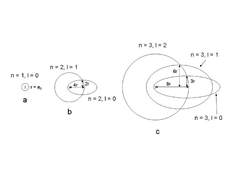
Figure 1: Bohr-Sommerfeld electron orbits for $n=1$, $2$, and $3$, and the allowed values for $l$.

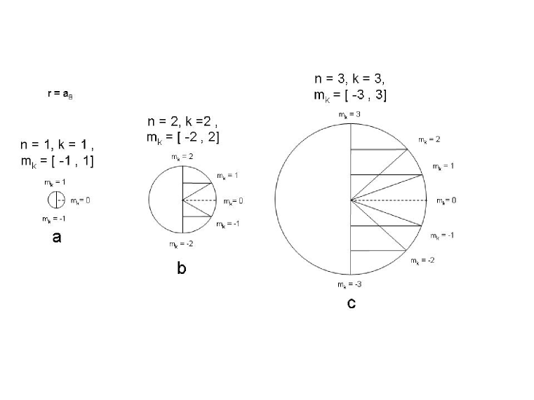
Figure 2: Spatial quantization of Bohr-Sommerfeld orbits for azimuthal numbers $k$ = 1,2, and 3.

2.4 Experimental Proof of the Existence of Atomic Stationary States

The existence of discrete atomic energy levels was evidenced for the first time by J. Franck and G. Hertz in 1914 [5]. They observed that when an electron collides with an atom (mercury in their case), a transfer of a particular amount of energy occurred. This energy transfer was recorded spectroscopically and confirmed Bohr’s hypotheses that atoms can absorb energy only in quantum portions. Even today, the experiment is preferentially done either with mercury or neon tubes. From the spectroscopic evidence, it is known that the excited mercury vapor emits ultraviolet radiation whose wavelength is 2536 Å, corresponding to a photon energy $h\nu$ equal to 4.89 eV.

The famous Franck-Hertz curves represent the electron current versus the accelerating potential, shown in Fig. 3. The current shows a series of equally spaced maxima (and minima) at the distance of $\sim$ 4.9 V. The first dip corresponds to electrons that lose all their kinetic energy after one inelastic collision with a mercury atom, which is then promoted to its first excited state. The second dip corresponds to those electrons that have the double amount of kinetic energy and loses it through two inelastic collisions with two mercury atoms, and so on. All these excited atoms emit the same radiation at $\sim$ 2536 Å. But which is the ‘first’ excited state of mercury? It is spectroscopically denoted by ${}^{3}P_{1}$ in Fig. (4). Notice that the other two $P$ states cannot decay to the ground state ${}^{1}S_{0}$ because the dipole emission is forbidden for them and therefore they are termed metastable. More details, such that the observed peak separation depends on the geometry of the tube and the Hg vapor pressure, are explained in the readable paper of Hanne [6].

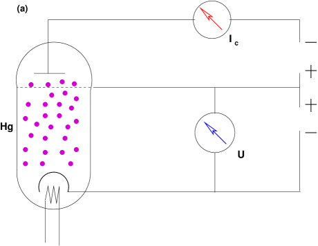
Figure 3: (a) Schematic diagram of the Franck-Hertz experiment, where the tube is filled with a gas of Mercury ; (b) typical plot recorded in a Franck-Hertz experiment with mercury, showing the periodic maxima.

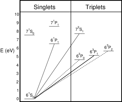
Figure 4: Simplified Mercury’s level diagram in the low-energy region in which the so-called hyperfine structure is neglected. The numbers 6 and 7 are Bohr’s ‘whole numbers’ or Schrödinger’s principal quantum numbers.

3 Stationary States in Wave Mechanics

3.1 The Schrödinger Equation

According to L. Pauling and E. Bright Wilson Jr. [7], already in the years 1920-1925 a decline of the ‘old quantum theory’ as the Bohr-Sommerfeld atomic theory is historically known and which is based on the ‘whole number’ quantization of cyclic orbits was patent; only very recently there is some revival, especially in the molecular context [8]. But in 1925, a quantum mechanics based on the matrix calculus was developed by W. Heisenberg, M. Born, and P. Jordan and the best was to come in 1926 when Schrödinger in a series of four papers developed the most employed form of quantum mechanics, known as wave mechanics. The advantage of his theory of atomic motion is that it is based on standard (partial) differential equations, more exactly on the Sturm-Liouville theory of self-adjoint linear differential operators. Schrödinger starts the first paper in the 1926 series with the following sentence [9]:

In this paper I wish to consider, first the simplest case of the hydrogen atom, and show that the customary quantum conditions can be replaced by another postulate, in which the notion of ‘whole numbers’, merely as such, is not introduced.

Indeed, he could obtain the basic equation of motion in nonrelativistic quantum mechanics, the so called Schrödinger equation for the wavefunctions $\Psi(x,t)$, and provided several analytic applications, among which was the hydrogen atom. The original derivation is based on the variational calculus within the Sturm-Liouville approach and was given eighty years ago. In his first paper of 1926, Schrödinger states that the wavefunctions $\Psi$ should be such as to make the ‘Hamilton integral’

$${\cal J}_{S}[\Psi]=\int\left(\hbar^{2}T(q,\partial\psi/\partial q)+\Psi^{2}V\right)d\tau\ ,$$ (9)

stationary subject to the normalizing condition $\int\Psi^{2}d\tau=1$ which can be incorporated through the Lagrange multipliers method. The Euler-Lagrange equation of the functional ${\cal J}_{S}[\Psi]$ is the time-dependent Schrödinger equation

$$i\hbar\frac{\partial\Psi}{\partial t}=H\Psi~{}.$$ (10)

When the wave function of the time-dependent Schrödinger equation is written in the multiplicative form $\Psi(x,t)=\psi(x){\cal F}(t)$ one obtains a complete separation of the space and time behaviors of $\Psi$: on one side, one gets the stationary Schrödinger equation for $\psi(x)$,

$$-\frac{h^{2}}{2m}\frac{d^{2}\psi}{dx^{2}}+V(x)\psi=E\psi~{},$$ (11)

and on the other side, the simple time-dependent equation for the logderivative of ${\cal F}$

$$i\hbar\frac{d\log{\cal F}}{dt}=E$$ (12)

This decoupling of space and time components is possible whenever the potential energy is independent of time.

The space component has the form of a standing-wave equation. Thus, it is correct to regard the time-independent Schrödinger equation as a wave equation from the point of view of the spatial phenomenology.

3.2 The Dynamical Phase

Furthermore, the time-dependence is multiplicative and reduces to a modulation of the phase of the spatial wave given by

$${\cal F}=e^{-iEt/\hbar}=\cos(Et/\hbar)-i\sin(Et/\hbar)~{}.$$ (13)

The phase factor ${\cal F}=e^{-iEt/\hbar}$ is known as the dynamical phase. In recent times, other parametric phases have been recognized to occur, e.g., the Berry phase. The dynamical phase is a harmonic oscillation with angular frequency $\omega=E/h$ and period $T=h/E$. In other words, a Schrödinger wavefunction is flickering from positive through imaginary to negative amplitudes with a frequency proportional to the energy. Although it is a wave of constant energy it is not stationary because its phase is time dependent (periodic). However, a remarkable fact is that the product $\Psi^{*}\Psi$, i.e., the modulus $|\Psi|^{2}$ of the Schrödinger constant-energy waves remains constant in time

$$\Psi^{*}\Psi=\psi^{*}\psi$$ (14)

It is in the sense of their constant modulus that Schrödinger constant-energy waves are called stationary states.

3.3 The Schrödinger Wave Stationarity

Thus, non-relativistic quantum stationarity refers to waves of constant energy and constant modulus, but not of constant phase, which can occur as solutions of Schrödinger equation for time-independent potentials. In the Schrödinger framework, the dynamical systems are usually assumed to exist in stationary states (or waves of this type). It is worth noting that the preferred terminology is that of states and not of waves. This is due to the fact that being of constant energy the Schrödinger stationary waves describe physical systems in configurations (or states) of constant energy which can therefore be naturally associated to the traditional conservative Hamiltonian systems. Moreover, the localization of these waves can be achieved by imposing appropriate boundary conditions.

3.4 Stationary Schrödinger States and Classical Orbits

In the Schrödinger theory, a single stationary state does not correspond to a classical orbit. This is where the Schrödinger energy waves differ the most from Bohr’s theory which is based on quantized classical cyclic trajectories. To build a wave entity closer to the concept of a classical orbit, one should use superpositions of many stationary states, including their time dependence, i.e., what is known as wave packets. Only monochromatic plane waves of angular frequency $\omega$ corresponds through the basic formula $E=\hbar\omega$ to a well-defined energy $E$ of the ‘classical’ particle but unfortunately there is no relationship between the wavevector $k$ and the momentum $p$ of the corresponding particle since a plane wave means only the propagation at constant (phase) velocity of infinite planes of equal phase. In other words, a criterium for localization is required in order to define a classical particle by means of a wave approach.

In the one-dimensional case, a wave packet is constructed as follows

$$\psi(x,t)=\int_{-\infty}^{+\infty}f(k^{\prime})e^{i(k^{\prime}x-\omega^{\prime}t)}dk^{\prime}\ ,$$ (15)

with obvious generalization to more dimensions. If $f(k^{\prime})$ is written in the polar form $F(k^{\prime})e^{i\alpha}$ and $F$ is chosen with a pronounced peak in a wavenumber region of extension $\Delta k$ around the point $k^{\prime}=k$, then the wave packet is localized in a spatial region of extension $\Delta x\approx\frac{1}{\Delta k}$ surrounding the “center of the wavepacket”. The latter is equivalent to the concept of material point in classical mechanics and travels uniformly with the group velocity $v_{g}=\frac{d\omega}{dk}$. This is the velocity that can be identified with the particle velocity $v=\frac{dE}{dp}$ in classical mechanics and which leads to the de Broglie formula $p=\hbar k=\frac{h}{\lambda}$.

3.5 Stationary States as Sturm-Liouville Eigenfunctions

The mathematical basis of Schrödinger wave mechanics is the Sturm-Liouville (SL) theory of self-adjoint linear differential operators established in the 19th century, more specifically the SL eigenvalue problem, which is to find solutions of a differential equation of the form

$${\cal L}u_{n}(x)\equiv\frac{d}{dx}\left[p(x)\frac{du_{n}(x)}{dx}\right]-q(x)u_{n}(x)=-\mu_{n}w(x)u_{n}(x)$$ (16)

subject to specified boundary conditions at the beginning and end of some interval $(a,b)$ on the real line, e.g.

$$Au(a)+Bu^{\prime}(a)=0$$ (17)

$$Cu(b)+Du^{\prime}(b)=0$$ (18)

where $A,B,C,D$ are given constants. The differential operator ${\cal L}$ in (16) is rather general since any second order linear differential operator can be put in this form after multiplication by a suitable factor. The boundary conditions are also rather general including the well-known Dirichlet and Neumann boundary conditions as particular cases but other possibilities such as periodic boundary conditions

$$u(x)=u(x+b-a)$$ (19)

could be of interest in some cases, especially for angular variables.

The SL eigenvalue problem is an infinite dimensional generalization of the finite dimensional matrix eigenvalue problem

$$Mu=\mu u$$ (20)

with $M$ an $n\times n$ matrix and $u$ an $n$ dimensional column vector. As in the matrix case, the SL eigenvalue problem will have solutions only for certain values of the eigenvalue $\mu_{n}$. The solutions $u_{n}$ corresponding to these $\mu_{n}$ are the eigenvectors. For the finite dimensional case with an $n\times n$ matrix $M$ there can be at most $n$ linearly independent eigenvectors. For the SL case there will in general be an infinite set of eigenvalues $\mu_{n}$ with corresponding eigenfunctions $u_{n}(x)$.

The differential equations derived by separating variables are in general of the SL form, the separation constants being the eigenvalue parameters $\mu$. The boundary conditions (17,18) are determined by the physical application under study.

The solutions $u_{n}(x),\,\mu_{n}$ of a SL eigenvalue problem have some general properties of basic importance in wave (quantum) mechanics.

If $u(x)$ and $v(x)$ are arbitrary twice differentiable solutions of a SL operator, then by integrating by parts

$$\int_{a}^{b}dx[v{\cal L}u-u{\cal L}v]=p\left(v\frac{du}{dx}-u\frac{dv}{dx}\right)\bigg{|}_{a}^{b}~{}.$$ (21)

An operator ${\cal L}$ which satisfies (21) is said to be self-adjoint. Any second order linear differential operator can be put in this self adjoint form by multiplication by a suitable factor.

It is easy to show that for functions $u(x)$, $v(x)$ satisfying boundary conditions of the standard SL form or the periodic boundary condition (19) the right hand side of (21) vanishes. For both of this case we then have

$$\int_{a}^{b}dxv{\cal L}u=\int_{a}^{b}dxu{\cal L}v~{}.$$ (22)

Consider now two different eigenfunctions $u_{n}(x)$, $u_{m}(x)$ belonging to different eigenvalues $\lambda_{n}\neq\lambda_{m}$:

$${\cal L}u_{n}(x) = -\mu_{n}w(x)u_{n}(x)~{},$$ (23)

$${\cal L}u_{m}(x) = -\mu_{m}w(x)u_{m}(x)~{}.$$ (24)

Multiplying the first equation by $u_{m}$ and the second one by $u_{n}$, integrating and subtracting, we find:

$$\int_{a}^{b}dx[u_{m}{\cal L}u_{n}-u_{n}Lu_{m}]=-(\mu_{n}-\mu_{m})\int_{a}^{b}dxw(x)u_{n}(x)u_{m}(x)~{}.$$ (25)

The left hand side will vanish for either set of boundary conditions we consider here, so for either of these cases, we find the orthogonality condition

$$\int_{a}^{b}dxw(x)u_{n}(x)u_{m}(x)=0~{},\qquad\mu_{n}\neq\mu_{m}~{}.$$ (26)

Two functions $u_{n}(x)$, $u_{m}(x)$ satisfying this condition are said to be orthogonal with weight $w(x)$. Moreover, if $w(x)$ is non negative, one can introduce the SL normalization of the $u_{n}$ as follows:

$$\int_{a}^{b}dxw(x)[u_{n}(x)]^{2}=1~{}.$$ (27)

The most important property of the eigenfunctions of a SL problem is that they form a complete set. This means that an arbitrary function $\psi(x)$ can be expanded in an infinite series of the form

$$\psi(x)=\sum_{n}a_{n}u_{n}(x)~{}.$$ (28)

The expansion coefficients $a_{n}$ are determined by multiplying (28) by $w(x)u_{n}(x)$, integrating term by term, and using the orthogonality relation

$$a_{n}=\frac{\int_{a}^{b}dxw(x)u_{n}(x)\psi(x)}{\int_{a}^{b}dxw(x)[u_{n}(x)]^{2}}~{}.$$ (29)

According to Courant and Hilbert [10], every piecewise continuous function defined in some domain with a square-integrable first derivative may be expanded in an eigenfunction series which converges absolutely and uniformly in all subdomains free of points of discontinuity; at the points of discontinuity it represents (like the Fourier series) the arithmetic mean of the right and left hand limits. (This theorem does not require that the functions expanded satisfy the boundary conditions.)

4 The Infinite Square Well: The Stationary States Most Resembling the Standing Waves on a String

We have already commented that the time-independent Schrödinger equation has the form of a standing-wave equation. This is a very instructive analogy and allows to obtain the correct energy values for the case of the infinite square well using only the de Broglie wave concept without even introducing the Schrödinger equation [11].

We remind the treatment of the string standing waves in the case of a finite homogeneous string of total length $L$. Provided that the origin of the coordinate system is placed in its center and the $x$ direction is chosen parallel to it, the space dependent part of its standing waves is given by

$$u(x)=A\cos kx+B\sin kx$$ (30)

where $x\in(-L/2,L/2)$ and $A$, $B$, and $k$ are constants. Imposing the usual (Dirichlet) boundary conditions

$$u(-L/2)=u(L/2)=0\ ,$$ (31)

equation (30) takes the form

$$u_{n}(x)=\left\{\begin{array}[]{ll}A\cos k_{n}x~{},&\mbox{if $n>0$ and odd}\\ B\sin k_{n}x~{},&\mbox{if $n>0$ and even}\end{array}\right.$$ (32)

where

$$x\in(-L/2,L/2)$$ (33)

and

$$k_{n}=\frac{n\pi}{L}~{},\qquad(n=1,2,3,...)~{}.$$ (34)

These functions - the normal modes of the string under consideration - form a complete set with respect to physically reasonable functions defined within the interval (33) and satisfying equation (31), i.e., any such function $U(x)$ can be written as the Fourier series

$$U(x)=\sum_{n=1}^{\infty}c_{n}u_{n}(x)~{}.$$ (35)

We are ready now to state the analogy, which is based on the following steps.

• A standing de Broglie wave corresponds to a quantum particle strictly confined to the region $-L/2\leq x\leq L/2$, i.e., in an infinite square-well potential shown in (Fig. (5)

  $$V(x)=\left\{\begin{array}[]{ll}0~{},&\mbox{if $|x|\leq L/2$}\\ -\infty~{},&\mbox{if $|x|>L/2~{}.$}\end{array}\right.$$ (36)

  

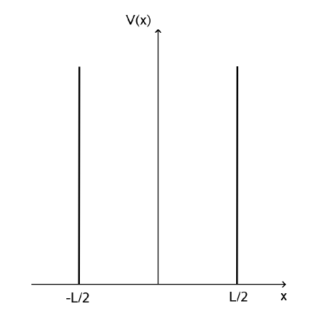
  Figure 5: The infinite square well potential. This case is mathematically the most analogous to the classical string standing waves.

  Because of the form of this potential, it is assumed that there is no asymptotic tail of the wave functions in the outside regions to the well, i.e., $\psi(x)=0$ for $|x|>L/2$. In physical terms, that means that the particle is completely localized within the wall and the boundary conditions are of the Dirichlet type.

  In the interior region, the Schrödinger equation is the simplest possible:

  $$-\frac{h^{2}}{2m}\frac{d^{2}\psi}{dx^{2}}-E\psi=0\ ,$$ (37)

  whose solutions (energy eigenfunctions) are:

  $$\phi_{n}(x)=\left\{\begin{array}[]{lll}(2/L)^{1/2}\sin(n\pi x/L)~{},&n\,\mbox{even}~{},\quad\mbox{$|x|\leq L/2$}\ ,\\ (2/L)^{1/2}\cos(n\pi x/L)~{},&n\,\mbox{odd}~{},\quad\mbox{$|x|\leq L/2$}\ ,\\ 0~{},&\quad\mbox{$|x|>L/2~{},$}\end{array}\right.$$ (38)

  and the energy eigenvalues are:

  $$E_{n}=\frac{(\hbar k_{n})^{2}}{2m}=\frac{\hbar^{2}\pi^{2}n^{2}}{2mL^{2}}~{}.$$ (39)

• The amplitude of this standing wave in the $n$th stationary state is proportional to $\sin(n\pi z/L)$. This corresponds strictly to the analogy with standing waves on a classical string.

• The $n$th standing wave is presented as a superposition of two running waves. The wave travelling right, with wavelength $\lambda_{n}=2L/n$ has de Broglie momentum $\hbar\pi n/L$ and the left travelling wave has opposed de Broglie momentum $-\hbar\pi n/L$. The resulting energy is then quantized and given by

  $$E_{n}=\frac{p_{n}^{2}}{2m}=\frac{\hbar^{2}\pi^{2}n^{2}}{2mL^{2}}~{}.$$ (40)

Because of the extremely strong confinement of the infinite square well it seems that this case is only of academic interest. However, two-dimensional strong confinement of electrons by rings of adatoms (corrals) have been reported in the literature [12].

5 1D Parabolic Well: The Stationary States of the Quantum Harmonic Oscillator

5.1 The Solution of the Schrödinger Equation

The harmonic oscillator (HO) is one of the fundamental paradigms of Physics. Its utility resides in its simplicity which is manifest in many areas from classical physics to quantum electrodynamics and theories of gravitational collapse.
It is well known that within classical mechanics many complicated potentials can be well approximated close to their equilibrium positions $a_{i}$ by HO potentials as follows

$$V(x)\sim\frac{1}{2}V^{\prime\prime}(a_{i})(x-a_{i})^{2}~{}.$$ (41)

For this case, the classical Hamiltonian function of a particle of mass m, oscillating at the frequency $\omega$ has the following form:

$$H=\frac{p^{2}}{2m}+\frac{1}{2}m\omega^{2}x^{2}\ ,$$ (42)

and the quantum Hamiltonian corresponding to the configurational space is given by

$$\hat{H}=\frac{1}{2m}\left(-i\hbar\frac{d}{dx}\right)^{2}+\frac{1}{2}m\omega^{2}x^{2}=-\frac{\hbar^{2}}{2m}\frac{d^{2}}{dx^{2}}+\frac{1}{2}m\omega^{2}x^{2}~{}.$$ (43)

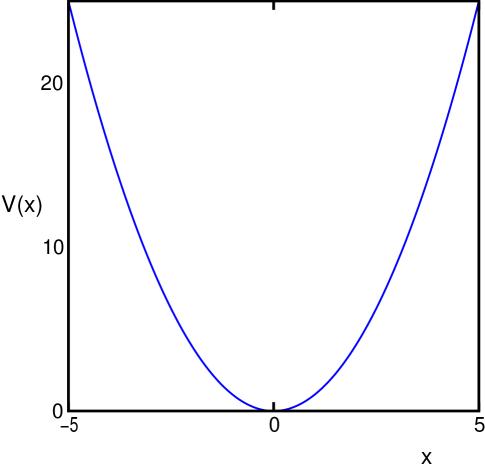
Figure 6: The harmonic (parabolic) oscillator potential.

Since we consider a time-independent potential, the eigenfunctions $\psi_{n}$ and the eigenvalues $E_{n}$ are obtained by means of the time-independent Schrödinger equation

$$\hat{H}\psi=E\psi~{}.$$ (44)

For the HO Hamiltonian, the Schrödinger equation is

$$\frac{d^{2}\psi}{dx^{2}}+\Bigg{[}\frac{2mE}{\hbar^{2}}-\frac{m^{2}\omega^{2}}{\hbar^{2}}x^{2}\Bigg{]}\psi=0~{}.$$ (45)

Defining the parameters

$$k^{2}=\frac{2mE}{\hbar^{2}}~{},\qquad\lambda=\frac{m\omega}{\hbar}~{},$$ (46)

the Schrödinger equation becomes

$$\frac{d^{2}\Psi}{dx^{2}}+[k^{2}-\lambda^{2}x^{2}]\Psi=0~{},$$ (47)

which is known as Weber’s differential equation in mathematics. To solve this equation one makes use of the following variable transformation

$$y=\lambda x^{2}~{}.$$ (48)

By changing the independent variable from $x$ to $y$, the differential operators $D_{x}$ and $D_{x}^{2}$ take the form

$$D_{x}\equiv\frac{d}{dx}=\left(\frac{dy}{dx}\right)D_{y}~{},\quad D_{x}^{2}\equiv\frac{d^{2}}{dx^{2}}=\frac{d}{dx}\left(\frac{dy}{dx}\frac{d}{dy}\right)=\left(\frac{d^{2}y}{dx^{2}}\right)D_{y}+\left(\frac{dy}{dx}\right)^{2}D_{y}^{2}~{}.$$ (49)

By applying these rules to the proposed transformation we obtain the following differential equation in the $y$ variable

$$y\frac{d^{2}\psi}{dy^{2}}+\frac{1}{2}\frac{d\psi}{dy}+\left[\frac{k^{2}}{4\lambda}-\frac{1}{4}y\right]\psi=0~{},$$ (50)

and, by defining:

$$\kappa=\frac{k^{2}}{2\lambda}=\frac{E}{\hbar\omega}~{},$$ (51)

we get after dividing by $y$ (i.e., $y\neq 0$)

$$\frac{d^{2}\psi}{dy^{2}}+\frac{1}{2y}\frac{d\psi}{dy}+\left[\frac{\kappa}{2y}-\frac{1}{4}\right]\psi=0~{}.$$ (52)

Let us try to solve this equation by first doing its asymptotic analysis in the limit $y\rightarrow\infty$ in which the equation behaves as follows

$$\frac{d^{2}\psi_{\infty}}{dy^{2}}-\frac{1}{4}\psi_{\infty}=0~{}.$$ (53)

This equation has as solution

$$\psi_{\infty}(y)=A\exp\left(\frac{y}{2}\right)+B\exp\left(-\frac{y}{2}\right)~{}.$$ (54)

The first term diverges in the limit $y\rightarrow\infty$. Thus we take $A=0$, and keep only the attenuated exponential. We can now suggest that $\psi$ has the following form

$$\psi(y)=\exp\left(-\frac{y}{2}\right)\varphi(y)~{}.$$ (55)

Plugging it in the differential equation for $y$ ( Eq. (52)) one gets:

$$y\frac{d^{2}\varphi}{dy^{2}}+\left(\frac{1}{2}-y\right)\frac{d\varphi}{dy}+\left(\frac{\kappa}{2}-\frac{1}{4}\right)\varphi=0~{}.$$ (56)

The latter equation is of the confluent (Kummer) hypergeometric form

$$z\frac{d^{2}f}{dz^{2}}+(c-z)\frac{df}{dz}-af=0~{},$$ (57)

whose general solution is

$$f(z)=A\hskip 5.69046pt_{1}F_{1}(a,c;z)+B\hskip 5.69046ptz^{1-c}\hskip 2.84544pt_{1}F_{1}(a-c+1,2-c;z)~{},$$ (58)

where the confluent hypergeometric function is defined as follows

$$_{1}F_{1}(a,c;z)=\sum_{n=0}^{\infty}\frac{(a)_{n}z^{n}}{(c)_{n}n!}~{}.$$ (59)

By direct comparison of Eqs. (57) and (56), one can see that the general solution of the latter one is

$$\varphi(y)=A\hskip 5.69046pt_{1}F_{1}\left(a,\frac{1}{2};y\right)+B\hskip 5.69046pty^{\frac{1}{2}}\hskip 5.69046pt_{1}F_{1}\left(a+\frac{1}{2},\frac{3}{2};y\right)~{},$$ (60)

where

$$a=-\left(\frac{\kappa}{2}-\frac{1}{4}\right)~{}.$$ (61)

If we keep these solutions in their present form, the normalization condition is not satisfied by the wavefunction. Indeed, because the $|y|\rightarrow\infty$ asymptotic behaviour of the confluent hypergeometric function is ${}_{1}F_{1}(a,c;y)\rightarrow\frac{\Gamma(c)}{\Gamma(c-a)}e^{-ia\pi}y^{-a}+\frac{\Gamma(c)}{\Gamma(a)}e^{y}y^{a-c}$, it follows from the dominant exponential behavior that:

$$\psi(y)=e^{(-\frac{y}{2})}\varphi(y)\rightarrow\hskip 8.5359pt{\rm const.}\hskip 5.69046pte^{(\frac{y}{2})}y^{a-\frac{1}{2}}~{}.$$ (62)

This leads to a divergence in the normalization integral, which physically is not acceptable. What one does in this case is to impose the termination condition for the series. That is, the series is cut to a finite number of $n$ terms and therefore turns into a polynomial of order $n$. The truncation condition of the confluent hypergeometric series ${}_{1}F_{1}(a,c;z)$ is $a=-n$, where $n$ is a nonnegative integer (i.e., zero is included).
We thus notice that asking for a finite normalization constant, (as already known, a necessary condition for the physical interpretation in terms of probabilities), leads us to the truncation of the series, which simultaneously generates the quantization of energy.
In the following we consider the two possible cases:

$1)\hskip 11.38092pta=-n\hskip 8.5359pt$ and $B=0$

$$\frac{\kappa}{2}-\frac{1}{4}=n~{}.$$ (63)

The eigenfunctions are given by

$$\psi_{n}(x)={\cal N}_{n}\exp\left(\frac{-\lambda x^{2}}{2}\right)\hskip 2.84544pt_{1}F_{1}\left(-n,\frac{1}{2};\lambda x^{2}\right)$$ (64)

and the energy is:

$$E_{n}=\hbar\omega\left(2n+\frac{1}{2}\right)~{}.$$ (65)

$2)\hskip 11.38092pta+\frac{1}{2}=-n\hskip 8.5359pt$ and $A=0$

$$\frac{\kappa}{2}-\frac{1}{4}=n+\frac{1}{2}~{}.$$ (66)

The eigenfunctions are now

$$\psi_{n}(x)={\cal N}_{n}\exp\left(-\frac{\lambda x^{2}}{2}\right)\hskip 5.69046ptx\hskip 5.69046pt_{1}F_{1}\left(-n,\frac{3}{2};\lambda x^{2}\right)~{},$$ (67)

whereas the stationary energies are

$$E_{n}=\hbar\omega\left[(2n+1)+\frac{1}{2}\right]~{}.$$ (68)

The polynomials obtained by this truncation of the confluent hypergeometric series are called Hermite polynomials and in hypergeometric notation they are

$$H_{2n}(\eta) = (-1)^{n}\frac{(2n)!}{n!}\hskip 5.69046pt_{1}F_{1}\left(-n,\frac{1}{2};\eta^{2}\right)\ ,$$ (69)

$$H_{2n-1}(\eta) = (-1)^{n}\frac{2(2n+1)!}{n!}\hskip 5.69046pt\eta\hskip 5.69046pt_{1}F_{1}\left(-n,\frac{3}{2};\eta^{2}\right)~{}.$$ (70)

We can now combine the obtained results (because some of them give us the even cases and the others the odd ones) in a single expression for the oscillator eigenvalues and eigenfunctions

$$\psi_{n}(x) = {\cal N}_{n}\exp\left(-\frac{\lambda x^{2}}{2}\right)H_{n}(\sqrt{\lambda}x)$$ (71)

$$E_{n} = \left(n+\frac{1}{2}\right)\hbar\omega\hskip 28.45274ptn=0,1,2~{}\ldots$$ (72)

The HO energy spectrum is equidistant, i.e., there is the same energy difference $\hbar\omega$ between any consecutive neighbor levels. Another remark refers to the minimum value of the energy of the oscillator; somewhat surprisingly it is not zero. This is considered by many people to be a pure quantum result because it is zero when $\hbar\rightarrow 0$. $E_{0}=\frac{1}{2}\hbar\omega$ is known as the zero point energy and the fact that it is nonzero is the main characteristic of all confining potentials.

5.2 The Normalization Constant

The normalization constant is usually calculated in the following way. The Hermite generating function $e^{\lambda(-t^{2}+2tx)}$ is multiplied by itself and then by $e^{-\lambda x^{2}}$:

$$e^{-\lambda x^{2}}e^{\lambda(-s^{2}+2sx)}e^{\lambda(-t^{2}+2tx)}=\sum_{m,n=0}^{\infty}e^{-\lambda x^{2}}H_{m}(\sqrt{\lambda}x)H_{n}(\sqrt{\lambda}x)\frac{\lambda^{\frac{m+n}{2}}s^{m}t^{n}}{m!n!}~{}.$$ (73)

Integrating over $x^{\prime}=\sqrt{\lambda}x$ on the whole real line, the cross terms of the double sum drop out because of the orthogonality property

$$\sum_{n=0}^{\infty}\frac{\lambda^{n}(st)^{n}}{(n!)^{2}}\int_{-\infty}^{\infty}e^{-x^{\prime 2}}[H_{n}(x^{\prime})]^{2}dx^{\prime} = \int_{-\infty}^{\infty}e^{-x^{\prime 2}-s^{\prime 2}+2s^{\prime}x^{\prime}-t^{\prime 2}+2t^{\prime}x^{\prime}}dx^{\prime}=$$

$$=\int_{-\infty}^{\infty}e^{-(x^{\prime}-s^{\prime}-t^{\prime})^{2}}e^{2s^{\prime}t^{\prime}}dx^{\prime} = \pi^{1/2}e^{2st}=\pi^{1/2}\sum_{n=0}^{\infty}\frac{2^{n}\lambda^{n}(st)^{n}}{n!}$$

where the properties of the Euler gamma function have been used

$$\Gamma(z)=2\int_{0}^{\infty}e^{-t^{2}}t^{2z-1}dt~{},\qquad{\rm Re}(z)>0$$ (75)

as well as the particular case $z=1/2$ when $\Gamma(1/2)=\sqrt{\pi}$.

By equating coefficients of like powers of $st$ in (5.2), we obtain

$$\int_{-\infty}^{\infty}e^{-x^{\prime 2}}[H_{n}(x^{\prime})]^{2}dx^{\prime}=2^{n}\pi^{1/2}n!~{}.$$ (76)

This leads to

$${\cal N}_{n}=\Bigg{[}\sqrt{\frac{\lambda}{\pi}}\frac{1}{2^{n}n!}\Bigg{]}^{\frac{1}{2}}~{}.$$ (77)

5.3 Final Formulas for the HO Stationary States

Thus, one gets the following normalized eigenfunctions (stationary states) of the one-dimensional harmonic oscillator operator

$$\psi_{n}(x)=\Bigg{[}\sqrt{\frac{\lambda}{\pi}}\frac{1}{2^{n}n!}\Bigg{]}^{\frac{1}{2}}\hskip 5.69046pt\exp\left(\frac{-\lambda x^{2}}{2}\right)\hskip 5.69046ptH_{n}(\sqrt{\lambda}x)~{}.$$ (78)

If the dynamical phase factor ${\cal F}$ is included, the harmonic oscillator eigenfunctions takes the following final form

$$\psi_{n}(x,t)=\Bigg{[}\sqrt{\frac{\lambda}{\pi}}\frac{1}{2^{n}n!}\Bigg{]}^{\frac{1}{2}}\hskip 5.69046pt\exp\left(-i\left(n+\frac{1}{2}\right)\omega t-\frac{\lambda x^{2}}{2}\right)\hskip 5.69046ptH_{n}(\sqrt{\lambda}x)~{}.$$ (79)

5.4 The Algebraic Approach: Creation and Annihilation Operators $\hat{a}^{\dagger}$ and $\hat{a}$

There is another approach to deal with the HO besides the conventional one of solving the Schrödinger equation. It is the algebraic method, also known as the method of creation and annihilation (ladder) operators. This is a very efficient procedure, which can be successfully applied to many quantum-mechanical problems, especially when dealing with discrete spectra.
Let us define two nonhermitic operators $a$ and $a^{\dagger}$ :

$$a=\sqrt{\frac{m\omega}{2\hbar}}\left(x+\frac{ip}{m\omega}\right)\ ,$$ (80)

$$a^{\dagger}=\sqrt{\frac{m\omega}{2\hbar}}\left(x-\frac{ip}{m\omega}\right)~{}.$$ (81)

These operators are known as annihilation operator and creation operator, respectively (the reason of this terminology will be seen in the following.
Let us calculate the commutator of these operators

$$[a,a^{\dagger}]=\frac{m\omega}{2\hbar}\left[x+\frac{ip}{m\omega},x-\frac{ip}{m\omega}\right]=\frac{1}{2\hbar}(-i[x,p]+i[p,x])=1~{},$$ (82)

where we have used the commutator $[x,p]=i\hbar$. Therefore the annihilation and creation operators do not commute, since we have $[a,a^{\dagger}]=1$. Let us also introduce the very important number operator $\hat{N}$:

$$\hat{N}=a^{\dagger}a~{}.$$ (83)

This operator is hermitic as one can readily prove using $(AB)^{\dagger}=B^{\dagger}A^{\dagger}$:

$$\hat{N}^{\dagger}=(a^{\dagger}a)^{\dagger}=a^{\dagger}(a^{\dagger})^{\dagger}=a^{\dagger}a=\hat{N}~{}.$$ (84)

Considering now that

$$a^{\dagger}a=\frac{m\omega}{2\hbar}\left(x^{2}+\frac{p^{2}}{m^{2}\omega^{2}}\right)+\frac{i}{2\hbar}[x,p]=\frac{\hat{H}}{\hbar\omega}-\frac{1}{2}\ ,$$ (85)

we notice that the Hamiltonian can be written in a quite simple form as a linear function of the number operator

$$\hat{H}=\hbar\omega\left(\hat{N}+\frac{1}{2}\right)~{}.$$ (86)

The number operator bears this name because its eigenvalues are precisely the subindexes of the eigenfunctions on which it acts

$$\hat{N}|n\rangle=n|n\rangle~{},$$ (87)

where we have used Dirac’s ket notation $\psi_{n}=|n\rangle$.

Applying the number-form of the HO Hamiltonian in (86) to this ket, one gets

$$\hat{H}|n\rangle=\hbar\omega\left(n+\frac{1}{2}\right)|n\rangle~{},$$ (88)

which directly shows that the energy eigenvalues are given by

$$E_{n}=\hbar\omega\left(n+\frac{1}{2}\right)~{}.$$ (89)

Thus, this basic result is obtained through purely algebraic means.

It is possible to consider the ket $a^{\dagger}|n\rangle$ as an eigenket of that number operator for which the eigenvalue is raised by one unit. In physical terms, this means that an energy quanta has been produced by the action of $a^{\dagger}$ on the ket $|n\rangle$. This already explains the name of creation operator. Similar comments with corresponding conclusion can be inferred for the operator $a$ explaining the name of annihilation operator (an energy quanta is eliminated from the system when this operator is put into action).

Consequently, we have

$$a^{\dagger}|n\rangle=\sqrt{n+1}|n+1\rangle~{}.$$ (90)

For the annihilation operator, following the same procedure one can get the following relation

$$a|n\rangle=\sqrt{n}|n-1\rangle~{}.$$ (91)

Let us show now that the values of $n$ should be nonnegative integers. For this, we employ the positivity requirement for the norm of the state vector $a|n\rangle$. The latter condition tells us that the inner product of the vector with its adjoint $(a|n\rangle)^{\dagger}$ (= $\langle n|a^{\dagger}$) should always be nonnegative

$$(\langle n|a^{\dagger})\cdot(a|n\rangle)\geq 0~{}.$$ (92)

This relationship is in fact the expectation value of the number operator

$$\langle n|a^{\dagger}a|n\rangle=\langle n|\hat{N}|n\rangle=\langle n|a^{\dagger}\sqrt{n}|n-1\rangle=\langle n|\sqrt{n}\sqrt{n}|n\rangle=n\geq 0~{}.$$ (93)

Thus, $n$ cannot be negative. It should be a positive integer since, if that would not be the case, by applying iteratively the annihilation operator a sufficient number of times we would be led to imaginary and negative eigenvalues, which would be a contradiction to the positivity of the inner product.
It is possible to express the state $|n\rangle$ directly as a function of the ground state $|0\rangle$ using the $n$th power of the creation operator as follows:

$$|n\rangle=\left[\frac{(a^{\dagger})^{n}}{\sqrt{n!}}\right]|0\rangle~{},$$ (94)

which can be obtained by iterations.

One can also apply this method to get the eigenfunctions in the configuration space. To achieve this, we start with the ground state

$$a|0\rangle=0~{}.$$ (95)

In the $x$-representation, we have

$$\hat{a}\psi_{0}(x)=\sqrt{\frac{m\omega}{2\hbar}}\left(x+\frac{ip}{m\omega}\right)\psi_{0}(x)=0~{}.$$ (96)

Recalling the form of the momentum operator in this representation, we can obtain a differential equation for the wavefunction of the ground state. Moreover, introducing the oscillator length $x_{0}=\sqrt{\frac{\hbar}{m\omega}}=\frac{1}{\sqrt{\lambda}}$, we get

$$\left(x+x_{0}^{2}\frac{d}{dx}\right)\psi_{0}=0~{}.$$ (97)

This equation can be readily solved and the normalization to unity of the full line integral of the squared modulus of the solution leads to the physical wavefunction of the HO ground state

$$\psi_{0}(x)=\left(\frac{1}{\sqrt{\sqrt{\pi}x_{0}}}\right)e^{-\frac{1}{2}(\frac{x}{x_{0}})^{2}}~{}.$$ (98)

The rest of the eigenfunctions describing the HO excited states, can be obtained by employing iteratively the creation operator. The procedure is the following

$$\psi_{1} = a^{\dagger}\psi_{0}=\left(\frac{1}{\sqrt{2}x_{0}}\right)\left(x-x_{0}^{2}\frac{d}{dx}\right)\psi_{0}\ ,$$ (99)

$$\psi_{2} = \frac{1}{\sqrt{2}}(a^{\dagger})^{2}\psi_{0}=\frac{1}{\sqrt{2!}}\left(\frac{1}{\sqrt{2}x_{0}}\right)^{2}\left(x-x_{0}^{2}\frac{d}{dx}\right)^{2}\psi_{0}~{}.$$ (100)

By mathematical induction, one can show that

$$\psi_{n}(x)=\frac{1}{\sqrt{\sqrt{\pi}2^{n}n!}}\hskip 5.69046pt\frac{1}{x_{0}^{n+\frac{1}{2}}}\hskip 5.69046pt\left(x-x_{0}^{2}\frac{d}{dx}\right)^{n}\hskip 5.69046pte^{-\frac{1}{2}(\frac{x}{x_{0}})^{2}}~{}.$$ (101)

5.5 HO Spectrum Obtained from Wilson-Sommerfeld Quantization Condition

In the classical phase space, the equation $H=E$ for the harmonic oscillator when divided by $E$, i.e.,

$$\frac{p_{x}^{2}}{2mE}+\frac{m\omega_{0}^{2}x^{2}}{2E}=1\ ,$$ (102)

turns into the equation for an ellipse

$$\frac{x^{2}}{a^{2}}+\frac{p_{x}^{2}}{b^{2}}=1\ ,$$ (103)

where $a=\frac{1}{\omega_{0}}\sqrt{\frac{2E}{m}}$ and $b=\sqrt{2mE}$. Therefore, applying the Bohr-Sommerfeld quantization rule for this case

$$J=\oint p_{x}dx=\pi ab=\frac{2\pi E}{\omega_{0}}=2\pi\hbar n~{},$$ (104)

one obtains immediately the spectrum

$$E_{n}=n\hbar\omega_{0}\ ,$$ (105)

which is the quantum HO spectrum up to the zero-point energy.

6 The 3D Coulomb Well: The Stationary States of the Hydrogen Atom

The case of the Hydrogen atom corresponds in wave mechanics to an effective potential well that is the sum of the Coulomb well and the quantum centrifugal barrier as shown in Fig. (7). This result comes out from the technique of the separation of variables that is to be considered for any differential equation in more than one dimension. A very good introduction to this technique can be found in the textbook of Arfken and Weber [13]. In general, for $d$ variables there are $d-1$ separation constants.

In spherical coordinates, the Schrödinger equation $(\nabla^{2}_{r}+V(r))\psi({\bf r})=E\psi({\bf r})$ reads

$$\frac{1}{r^{2}}\frac{\partial}{\partial r}\left(r^{2}\frac{\partial\psi}{\partial r}\right)+\frac{1}{r^{2}\sin\theta}\frac{\partial}{\partial\theta}\left(\sin\theta\frac{\partial\psi}{\partial\theta}\right)+\frac{1}{r^{2}\sin^{2}\theta}\frac{\partial^{2}\psi}{\partial\phi^{2}}+\frac{2m}{\hbar^{2}}(E-u)\psi=0\ ,$$ (106)

that can be also written in the form

$$\sin^{2}\theta\frac{\partial}{\partial r}\left(r^{2}\frac{\partial\psi}{\partial r}\right)+\sin\theta\frac{\partial}{\partial\theta}\left(\sin\theta\frac{\partial\psi}{\partial\theta}\right)+\frac{\partial^{2}\psi}{\partial\phi^{2}}+\frac{2mr^{2}\sin^{2}\theta}{\hbar^{2}}\left(\frac{e^{2}}{4\pi\epsilon_{0}r}+E\right)\psi=0~{}.$$ (107)

This equation is a partial differential equation for the electron wavefunction $\psi(r,\theta,\phi)$ ‘within’ the atomic hydrogen. Together with the various conditions that the wavefunction $\psi(r,\theta,\phi)$ should fulfill [for example, $\psi(r,\theta,\phi)$ should have a unique value at any spatial point ($r,\theta,\phi$)], this equation specifies in a complete manner the stationary behavior of the hydrogen electron.

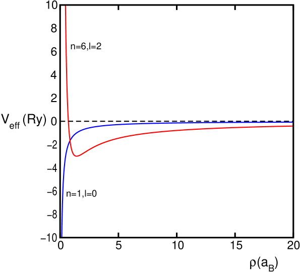
Figure 7: The effective potential well in the case of the hydrogen atom consisting of the electrostatic potential plus a quantized centrifugal barrier (see text).

6.1 The Separation of Variables in Spherical Coordinates

The real usefulness of writing the hydrogen Schrödinger equation in spherical coordinates consists in the easy way of achieving the separation procedure in three independent one-dimensional equations. The separation procedure is to seek the solutions for which the wavefunction $\psi(r,\theta,\phi)$ has the form of a product of three functions, each of one of the three spherical variables, namely $R(r)$ depending only on $r$, $\Theta(\theta)$ depending only on $\theta$, and $\Phi(\phi)$ that depends only on $\phi$. This is quite similar to the separation of the Laplace equation. Thus

$$\psi(r,\theta,\phi)=R(r)\Theta(\theta)\Phi(\phi)~{}.$$ (108)

The $R(r)$ function describes the differential variation of the electron wavefunction $\psi$ along the vector radius coming out from the nucleus, with $\theta$ and $\phi$ assumed to be constant. The differential variation of $\psi$ with the polar angle $\theta$ along a meridian of an arbitrary sphere centered in the nucleus is described only by the function $\Theta(\theta)$ for constant $r$ and $\phi$. Finally, the function $\Phi(\phi)$ describes how $\psi$ varies with the azimuthal angle $\phi$ along a parallel of an arbitrary sphere centered at the nucleus, under the conditions that $r$ and $\theta$ are kept constant.

Using $\psi=R\Theta\Phi$, one can see that

$$\frac{\partial\psi}{\partial r}=\Theta\Phi\frac{dR}{dr}~{},\qquad\frac{\partial\psi}{\partial\theta}=R\Phi\frac{d\Theta}{d\theta}~{},\qquad\frac{\partial\psi}{\partial\phi}=R\Theta\frac{d\Phi}{d\phi}~{}.$$ (109)

Then, one can obtain the following equations for the three factoring functions:

$$\frac{d^{2}\Phi}{d\phi^{2}}+m_{l}^{2}\Phi=0~{},$$ (110)

$$\frac{1}{\sin\theta}\frac{d}{d\theta}\left(\sin\theta\frac{d\Theta}{d\theta}\right)+\left[l(l+1)-\frac{m_{l}^{2}}{\sin^{2}\theta}\right]\Theta=0~{},$$ (111)

$$\frac{1}{r^{2}}\frac{d}{dr}\left(r^{2}\frac{dR}{dr}\right)+\left[\frac{2m}{\hbar^{2}}\left(\frac{e^{2}}{4\pi\epsilon_{0}r}+E\right)-\frac{l(l+1)}{r^{2}}\right]R=0~{}.$$ (112)

Each of these equations is an ordinary differential equation for a function of a single variable. In this way, the Schrödinger equation for the hydrogen electron, which initially was a partial differential equation for a function $\psi$ of three variables, gets a simple form of three 1D ordinary differential equations for unknown functions of one variable. The reason why the separation constants have been chosen as $-m_{l}^{2}$ and $-l(l+1)$ will become clear in the following subsections.

6.2 The Angular Separation Constants as Quantum Numbers

6.2.1 The Azimuthal Solution and the Magnetic Quantum Number

The Eq. (110) is easily solved leading to the following solution

$$\Phi(\phi)={\cal N}_{\Phi}e^{im_{l}\phi}~{},$$ (113)

where ${\cal N}_{\Phi}$ is the integration constant that will be used as a normalization constant for the azimuthal part. One of the conditions that any wavefunctions should fulfill is to have a unique value for any point in space. This applies to $\Phi$ as a component of the full wavefunction $\psi$. One should notice that $\phi$ and $\phi+2\pi$ must be identical in the same meridional plane. Therefore, one should have $\Phi(\phi)=\Phi(\phi+2\pi)$, i.e., ${\cal N}_{\Phi}e^{im_{l}\phi}={\cal N}_{\Phi}e^{im_{l}(\phi+2\pi)}$. This can be fulfilled only if $m_{l}$ is zero or a positive or negative integer $(\pm 1,\pm 2,\pm 3,...)$. The number $m_{l}$ is known as the magnetic quantum number of the atomic electron and is related to the direction of the projection of the orbital momentum $L_{z}$. It comes into play whenever the effects of axial magnetic fields on the electron may show up. There is also a deep connection between $m_{l}$ and the orbital quantum number $l$, which in turn determines the modulus of the orbital momentum of the electron.

The solution for $\Phi$ should also fulfill the normalization condition when integrating over a full period of the azimuthal angle,

$$\int_{0}^{2\pi}\mid\Phi\mid^{2}d\phi=1$$ (114)

and substituting $\Phi$, one gets

$$\int_{0}^{2\pi}{\cal N}_{\Phi}^{2}d\phi=1~{}.$$ (115)

It follows that ${\cal N}_{\Phi}=1/\sqrt{2\pi}$, and therefore the normalized $\Phi$ is

$$\Phi(\phi)=\frac{1}{\sqrt{2\pi}}e^{im_{l}\phi}~{}.$$ (116)

6.2.2 The Polar Solution and the Orbital Quantum Number

The solution of the $\Theta(\theta)$ equation is more complicated since it contains two separation constants which can be proved to be integer numbers. Things get easier if one reminds that the same Eq. (111) occurs also when the Helmholtz equation for the spatial amplitude profiles of the electromagnetic normal modes is separated in spherical coordinates. From this case we actually know that this equation is the associated Legendre equation for which the polynomial solutions are the associated Legendre polynomials

$$P_{l}^{m_{l}}(x)=(-1)^{m_{l}}(1-x^{2})^{m_{l}/2}\frac{d^{m_{l}}}{dx^{m_{l}}}P_{l}(x)=(-1)^{m_{l}}\frac{(1-x^{2})^{m_{l}/2}}{2^{l}l!}\frac{d^{m_{l}+l}}{dx^{{m_{l}+l}}}(x^{2}-1)^{l}~{}.$$ (117)

The function $\Theta(\theta)$ are a normalized form, $\Theta(\theta)={\cal N}_{\Theta}P_{l}^{m_{l}}$, of the associated Legendre polynomials

$$\Theta(\theta)=\sqrt{\frac{2l+1}{2}\frac{(l-m_{l})!}{(l+m_{l})!}}P_{l}^{m_{l}}(cos\theta)~{}.$$ (118)

For the purposes here, the most important property of these functions is that they exist only when the constant $l$ is an integer number greater or at least equal to $|m_{l}|$, which is the absolute value of $m_{l}$. This condition can be written in the form of the set of values available for $m_{l}$

$$m_{l}=0,\pm 1,\pm 2,...,\pm l~{}.$$ (119)

The condition that $l$ should be a positive integer can be seen from the fact that for noninteger values, the solution of Eq. (111) diverges for $\cos\theta=\pm 1$, while for physical reasons we require finite solutions in these limits. The other condition $l\geq|m_{l}|$ can be obtained from examining Eq. (117), where one can see a derivative of order $m_{l}+l$ applied to a polynomial of order $2l$. Thus $m_{l}+l$ cannot be greater than $2l$. On the other hand, the derivative of negative order are not defined and that of zero order is interpreted as the unit operator. This leads to $m_{l}\geq-l$.

The interpretation of the orbital number $l$ does have some difficulties. Let us examine the equation corresponding to the radial wavefunction $R(r)$. This equation rules only the radial motion of the electron, i.e., with the relative distance with respect to the nucleus along some guiding ellipses. However, the total energy of the electron $E$ is also present. This energy includes the kinetic electron energy in its orbital motion that is not related to the radial motion. This contradiction can be eliminated using the following argument. The kinetic energy $T$ has two parts: a pure radial one $T_{radial}$ and $T_{orbital}$, which is due to the closed orbital motion. The potential energy $V$ of the electron is the attractive electrostatic energy. Therefore, the electron total energy is

$$E=T_{radial}+T_{orbital}-\frac{e^{2}}{4\pi\epsilon_{0}r}~{}.$$ (120)

Substituting this expression of $E$ in Eq. (112) we get after some regrouping of the terms

$$\frac{1}{r^{2}}\frac{d}{dr}\left(r^{2}\frac{dR}{dr}\right)+\frac{2m}{\hbar^{2}}\left[T_{radial}+T_{orbital}-\frac{\hbar^{2}l(l+1)}{2mr^{2}}\right]R=0~{}.$$ (121)

If the last two terms in parentheses compensate each other, we get a differential equation for the pure radial motion. Thus, we impose the condition

$$T_{orbital}=\frac{\hbar^{2}l(l+1)}{2mr^{2}}~{}.$$ (122)

However, the orbital kinetic energy of the electron is $T_{orbital}=\frac{1}{2}mv_{orbital}^{2}$ and since the orbital momentum of the electron is $L=mv_{orbital}r$, we can express the orbital kinetic energy in the form

$$T_{orbital}=\frac{L^{2}}{2mr^{2}}~{}.$$ (123)

Therefore, we have

$$\frac{L^{2}}{2mr^{2}}=\frac{\hbar^{2}l(l+1)}{2mr^{2}}\ ,$$ (124)

and consequently

$$L=\sqrt{l(l+1)}\hbar~{}.$$ (125)

The interpretation of this result is that since the orbital quantum number $l$ is constrained to take the values $l=0,1,2,...,(n-1)$, the electron can only have orbital momenta specified by means of Eq. (125). As in the case of the total energy $E$, the angular momentum is conserved and gets quantized. Its natural unit in quantum mechanics is $\hbar=h/2\pi=1.054\times 10^{-34}$ J.s.

In the macroscopic planetary motion (putting aside the many-body features), the orbital quantum number is so large that any direct experimental detection of the quantum orbital momentum is impossible. For example, an electron with $l=2$ has an angular momentum $L=2.6\times 10^{-34}$ J.s., whereas the terrestrial angular momentum is $2.7\times 10^{40}$ J.s.!

A common notation for the angular momentum states is by means of the letter $s$ for $l=0$, $p$ for $l=1$, $d$ for $l=2$, and so on. This alphabetic code comes from the empirical spectroscopic classification in terms of the so-called series, which was in use before the advent of wave mechanics.

On the other hand, for the interpretation of the magnetic quantum number, we must take into account that the orbital momentum is a vector operator and therefore one has to specify its direction, sense, and modulus. $L$, being a vector, is perpendicular on the plane of rotation. The geometric rules of the vectorial products still hold, in particular the rule of the right hand: its direction and sense are given by the right thumb whenever the other four fingers point at the direction of rotation.

6.2.3 The Space Quantization

We have already seen the spatial quantization of the Bohr-Sommerfeld electron trajectories. But what significance can be associated to a direction and sense in the limited volume of the atomic hydrogen in Schrödinger wave mechanics ? The answer may be quick if we think that the rotating electron is nothing but a one-electron loop current that considered as a magnetic dipole has a corresponding magnetic field. Consequently, an atomic electron will always interact with an applied magnetic field ${\bf H}$. The magnetic quantum number $m_{l}$ specifies the spatial direction of $L$, which is determined by the component of $L$ along the direction of the external magnetic field. This effect is commonly known as the quantization of the space in a magnetic field.

If we choose the direction of the magnetic field as the $z$ axis, the component of $L$ along this direction is

$$L_{z}=m_{l}\hbar~{}.$$ (126)

The possible values of $m_{l}$ for a given value of $l$, go from $+l$ to $-l$, passing through zero, so that there are $2l+1$ possible orientations of the angular momentum $L$ in a magnetic field. When $l=0$, $L_{z}$ can be only zero; when$l=1$, $L_{z}$ can be $\hbar$, 0, or $-\hbar$; when $l=2$, $L_{z}$ takes only one of the values $2\hbar$, $\hbar$, 0, $-\hbar$, or $-2\hbar$, and so forth. It is worth mentioning that $L$ cannot be put exactly parallel or anti-parallel to ${\bf H}$, because $L_{z}$ is always smaller than the modulus $\sqrt{l(l+1)}\hbar$ of the total orbital momentum.

One should consider the atom/electron characterized by a given $m_{l}$ as having the orientation of its angular momentum $L$ determined relative to the external applied magnetic field.

In the absence of the external magnetic field, the direction of the $z$ axis is fully arbitrary. Therefore, the component of $L$ in any arbitrary chosen direction is $m_{l}\hbar$; the external magnetic field offers a preferred reference direction from the experimental viewpoint.

Why only the component $L_{z}$ is quantized ? The answer is related to the fact that $L$ cannot be put along a direction in an arbitrary way. There is a special precessional motion in which its ‘vectorial arrow’ moves always along a cone centered on the quantization axis such that its projection $L_{z}$ is $m_{l}\hbar$. The reason why this quantum precession occurs is different from the macroscopic planetary motion as it is due to the uncertainty principle. If $L$ would be fixed in space, in such a way that $L_{x}$, $L_{y}$ and $L_{z}$ would have well-defined values, the electron would have to be confined to a well-defined plane. For example, if $L$ would be fixed along the $z$ direction, the electron tends to maintain itself in the plane $xy$.

This can only occur in the case in which the component $p_{z}$ of the electron momentum is ‘infinitely’ uncertain. This is however impossible if the electron is part of the hydrogen atom. But since in reality just the component $L_{z}$ of $L$ together with $L^{2}$ have well defined values and $|L|>|L_{z}|$, the electron is not constrained to a single plane. If this would be the case, an uncertainty would exist in the coordinate $z$ of the electron. The direction of $L$ changes continuously so that the mean values of $L_{x}$ and $L_{y}$ are zero, although $L_{z}$ keeps all the time its value $m_{l}\hbar$. It is here where Heisenberg’s uncertainty principle helps to make a clear difference between atomic wave motion and Bohr-Sommerfeld quantized ellipses.

6.3 Polar and Azimuthal Solutions Set Together

The solutions of the azimuthal and polar parts can be unified within spherical harmonics functions that depend on both $\phi$ and $\theta$. This simplifies the algebraic manipulations of the full wave functions $\psi(r,\theta,\phi)$. Spherical harmonics are given by

$$Y_{l}^{m_{l}}(\theta,\phi)=(-1)^{m_{l}}\sqrt{\frac{2l+1}{4\pi}\frac{(l-m_{l})!}{(l+m_{l})!}}P_{l}^{m_{l}}(cos\theta)e^{im_{l}\phi}~{}.$$ (127)

The factor $(-1)^{m_{l}}$ does not produce any problem because the Schrödinger equation is linear and homogeneous. This factor is added for the sake of convenience in angular momentum studies. It is known as the Condon-Shortley phase factor and its effect is to introduce the alternated sequence of the signs $\pm$ for the spherical harmonics of a given $l$.

6.4 The Radial Solution and the Principal Quantum Number

There is no energy parameter in the angular equations and that is why the angular motion does not make any contribution to the hydrogen spectrum. It is the radial motion that determines the energy eigenvalues. The solution for the radial part $R(r)$ of the wave function $\psi$ of the hydrogen atom is somewhat more complicated although the presence of two separation constants, $E$ and $l$, point to some associated orthogonal polynomials. In the radial motion of the hydrogen electron significant differences with respect to the electrostatic Laplace equation do occur. The final result is expressed analytically in terms of the associated Laguerre polynomials (Schrödinger 1926). The radial equation can be solved exactly only when E is positive or for one of the following negative values $E_{n}$ (in which cases, the electron is in a bound stationary state within atomic hydrogen)

$$E_{n}=-{\rm Ry}\left(\frac{1}{n^{2}}\right)~{},$$ (128)

where ${\rm Ry}=-\frac{me^{4}}{32\pi^{2}\epsilon_{0}^{2}\hbar^{2}}=13.606$ eV is the Rydberg atomic energy unit connected with the spectroscopic Rydberg constant $R_{\infty}$ through Ry $=hcR_{\infty}$, whereas $n$ is a positive integer number called the principal quantum number. It gives the quantization of the electron energy in the hydrogen atom. This discrete atomic spectrum has been first obtained in 1913 by Bohr using semi-empirical quantization methods and next by Pauli and Schrödinger almost simultaneously in 1926.

Another condition that should be satisfied in order to solve the radial equation is that $n$ have to be strictly bigger than $l$. Its lowest value is $l+1$ for a given $l$. Vice versa, the condition on $l$ is

$$l=0,1,2,...,(n-1)\ ,$$ (129)

for given $n$.

The radial equation can be written in the form

$$r^{2}\frac{d^{2}R}{dr^{2}}+2r\frac{dR}{dr}+\left[\frac{2mE}{\hbar^{2}}r^{2}+\frac{2me^{2}}{4\pi\epsilon_{0}\hbar^{2}}r-l(l+1)\right]R=0~{}.$$ (130)

Dividing by $r^{2}$ and using the substitution $\chi(r)=rR$ to eliminate the first derivative $\frac{dR}{dr}$, one gets the standard form of the radial Schrödinger equation displaying the effective potential $U(r)=-{\rm const}/r+l(l+1)/r^{2}$ (actually, electrostatic potential plus quantized centrifugal barrier). These are necessary mathematical steps in order to discuss a new boundary condition, since the spectrum is obtained by means of the $R$ equation. The difference between a radial Schrödinger equation and a full-line one is that a supplementary boundary condition should be imposed at the origin ($r=0$). The Coulomb potential belongs to a class of potentials that are called weak singular for which ${\rm lim}_{r\rightarrow 0}\,U(r)r^{2}=0$. In these cases, one tries solutions of the type $\chi\propto r^{\nu}$, implying $\nu(\nu-1)=l(l+1)$, so that the solutions are $\nu_{1}=l+1$ and $\nu_{2}=-l$, just as in electrostatics. The negative solution is eliminated for $l\neq 0$ because it leads to a divergent normalization constant, nor did it respect the normalization at the delta function for the continuous part of the spectrum. On the other hand, the particular case $\nu_{2}=0$ is eliminated because the mean kinetic energy is not finite. The final conclusion is that $\chi(0)=0$ for any $l$.

Going back to the analysis of the radial equation for $R$, the first thing to do is to write it in nondimensional variables. This is performed by noticing that the only space and time scales that one can form on combining the three fundamental constants entering this problem, namely $e^{2}$, $m_{e}$ and $\hbar$ are the Bohr atomic radius $a_{B}=\hbar^{2}/me^{2}=0.529\cdot 10^{-8}$ cm. and the atomic time $t_{B}=\hbar^{3}/me^{4}=0.242\cdot 10^{-16}$ sec., usually known as atomic units. Employing these units, one gets

$$\frac{d^{2}R}{dr^{2}}+\frac{2}{r}\frac{dR}{dr}+\left[2E+\frac{2}{r}-\frac{l(l+1)}{r^{2}}\right]R=0~{},$$ (131)

where we are especially interested in the discrete part of the spectrum ($E<0$). The notations $n=1/\sqrt{-E}$ and $\rho=2r/n$ leads us to

$$\frac{d^{2}R}{d\rho^{2}}+\frac{2}{\rho}\frac{dR}{d\rho}+\left[\frac{n}{\rho}-\frac{1}{4}-\frac{l(l+1)}{\rho^{2}}\right]R=0~{}.$$ (132)

For $\rho\rightarrow\infty$, this equation reduces to $\frac{d^{2}R}{d\rho^{2}}=\frac{R}{4}$, having solutions $R\propto e^{\pm\rho/2}$. Because of the normalization condition only the decaying exponential is acceptable. On the other hand, the asymptotic at zero, as we already commented on, should be $R\propto\rho^{l}$. Therefore, we can write $R$ as a product of three radial functions $R=\rho^{l}e^{-\rho/2}F(\rho)$, of which the first two give the asymptotic behaviors, whereas the third is the radial function in the intermediate region. The latter function is of most interest because its features determine the energy spectrum. The equation for $F$ is

$$\rho\frac{d^{2}F}{d\rho^{2}}+(2l+2-\rho)\frac{dF}{d\rho}+(n-l-1)F=0~{}.$$ (133)

This is a particular case of confluent hypergeometric equation. It can be identified as the equation for the associated Laguerre polynomials $L_{n+l}^{2l+1}(\rho)$. Thus, the normalized form of $R$ is

$$R_{nl}(\rho)=-\frac{2}{n^{2}}\sqrt{\frac{(n-l-1)!}{2n[(n+l)!]^{3}}}e^{-\rho/2}\rho^{l}L_{n+l}^{2l+1}(\rho)~{},$$ (134)

where the following Laguerre normalization condition has been used

$$\int_{0}^{\infty}e^{-\rho}\rho^{2l+1}[L_{n+l}^{2l+1}(\rho)]^{2}d\rho=\frac{2n[(n+l)!]^{3}}{(n-l-1)!}~{}.$$ (135)

6.5 Final Formulas for the Hydrogen Atom Stationary States

We have now the solutions of all the equations depending on a single variable and therefore we can build the stationary wave functions for any electronic state of the hydrogen atom. They have the following analytic form

$$\psi(r,\theta,\phi)={\cal N}_{H}(\alpha_{n}r)^{l}e^{-\alpha_{n}r/2}L_{n+l}^{2l+1}(\alpha_{n}r)P_{l}^{m_{l}}(cos\theta)e^{im_{l}\phi}~{},$$ (136)

where

$${\cal N}_{H}=-\frac{2}{n^{2}}\sqrt{\frac{2l+1}{4\pi}\frac{(l-m_{l})!}{(l+m_{l})!}\frac{(n-l-1)!}{[(n+l)!]^{3}}},\qquad\alpha_{n}=2/na_{B}~{}.$$ (137)

Using the spherical harmonics, the solution is written as follows

$$\psi(r,\theta,\phi)=-\frac{2}{n^{2}}\sqrt{\frac{(n-l-1)!}{[(n+l)!]^{3}}}(\alpha_{n}r)^{l}e^{-\alpha_{n}r/2}L_{n+l}^{2l+1}(\alpha_{n}r)Y_{l}^{m_{l}}(\theta,\phi)~{}.$$ (138)

If the dynamical factor ${\cal F}$ is included, we get

$$\psi(r,\theta,\phi;t)=-\frac{2}{n^{2}}\sqrt{\frac{(n-l-1)!}{[(n+l)!]^{3}}}(\alpha_{n}r)^{l}e^{\left(-i\left(\frac{Ry}{\hbar}\right)\frac{t}{n^{2}}-\frac{r}{na_{B}}\right)}L_{n+l}^{2l+1}(\alpha_{n}r)Y_{l}^{m_{l}}(\theta,\phi)~{}.$$ (139)

The latter formulas may be considered as the final result for the Schrödinger solution of the hydrogen atom for any stationary electron state. Indeed, one can see explicitly both the asymptotic dependence and the two orthogonal and complete sets of functions, i.e., the associated Laguerre polynomials and the spherical harmonics that correspond to this particular case of linear partial second-order differential equation. For the algebraic approach to the hydrogen atom problem we recommend the paper of Kirchberg and collaborators [16] and the references therein. Finally, the stationary hydrogen eigenfunctions are characterized by a high degeneracy since they depend on three quantum numbers whereas the energy spectrum is only $n$-dependent. The degree of degeneracy is easily calculated if one notice that there are $2l+1$ values of $m_{l}$ for a given $l$ which in turn takes values from $0$ to $n-1$ for a given $n$. Thus, there are $\sum_{l=0}^{n-1}(2l+1)=n^{2}$ states of given energy. Not only the presence of many degrees of freedom is the cause of the strong degeneracy. In the case of the hydrogen atom the existence of the conserved Runge-Lenz vector (commuting operator)${\bf K}=(2me^{2})^{-1}[{\bf L}\times{\bf P}-{\bf P}\times{\bf L}]+{\bf r}/r$ introduces more symmetry into the problem and enhances the degeneracy. On the other hand, the one-dimensional quantum wavefunctions are not degenerate because they are characterized by a single discrete index. The general problem of degeneracies is nicely presented in a paper by Shea and Aravind [17].

6.6 Electronic Probability Density

In the Bohr model of the hydrogen atom, the electron rotates around the nucleus on circular or elliptic trajectories. It is possible to think of appropriate experiments allowing to “see” that the electron moves within experimental errors at the predicted radii $r_{n}=n^{2}a_{0}$ in the equatorial plane $\theta=90^{o}$, whereas the azimuthal angle may vary according to the specific experimental conditions.

It is in this case that the more general wave mechanics changes the conclusions of the Bohr model in at least two important aspects:

$\bullet$ First, one cannot speak about exact values of $r,\theta,\phi$ (and therefore of planetary trajectories), but only of relative probabilities to find the electron within a given infinitesimal region of space. This feature is a consequence of the wave nature of the electron.

$\bullet$ Secondly, the electron does not move around the nucleus in the classical conventional way because the probability density $|\psi|^{2}$ does not depend on time but can vary substantially as a function of the relative position of the infinitesimal region.

The hydrogen electron wave function $\psi$ is $\psi=R\Theta\Phi$, where $R=R_{nl}(r)$ describes the way $\psi$ changes with $r$ when the principal and orbital quantum numbers have the values $n$ and $l$, respectively. $\Theta=\Theta_{lm_{l}}(\theta)$ describes in turn how $\psi$ varies with $\theta$ when the orbital and magnetic quantum numbers have the values $l$ and $m_{l}$, respectively. Finally, $\Phi=\Phi_{m_{l}}(\phi)$ gives the change of $\psi$ with $\phi$ when the magnetic quantum number has the value $m_{l}$. The probability density $\mid\psi\mid^{2}$ can be written

$$\mid\psi\mid^{2}=\mid R\mid^{2}\mid\Theta\mid^{2}\mid\Phi\mid^{2}~{}.$$ (140)

Notice that the probability density $|\Phi|^{2}$, which measures the possibility to find the electron at a given azimuthal angle $\phi$, is a constant (does not depend on $\phi$). Therefore, the electronic probability density is symmetric with respect to the $z$ axis and independent on the magnetic substates (at least until an external magnetic field is applied). Consequently, the electron has an equal probability to be found in any azimuthal direction. The radial part $R$ of the wave function, contrary to $\Phi$, not only varies with $r$, but it does it differently for any different combination of quantum numbers $n$ and $l$. Figure (8) shows plots of $R$ as a function of $r$ for the states $1s$, $2s$, and $2p$. $R$ is maximum at the center of the nucleus ($r=0$) for all the $s$ states, whereas it is zero at $r=0$ for all the states of nonzero angular momentum.

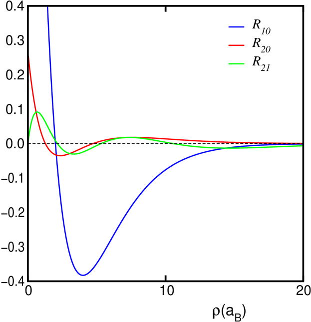
Figure 8: Approximate plots of the radial functions $R_{1s}$, $R_{2s}$, $R_{2p}$; ($a_{B}=0.53$ Å).

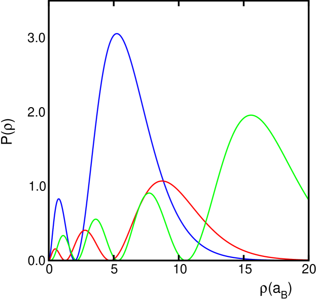
Figure 9: Probability density of finding the hydrogen electron between $r$ and $r+dr$ with respect to the nucleus for the states $1s$ (blue), $2s$ (red), $2p$ (green).

The electron probability density at the point $r,\theta,\phi$ is proportional to $|\psi|^{2}$, but the real probability in the infinitesimal volume element $dV$ is $\mid\psi\mid^{2}dV$. In spherical coordinates $dV=r^{2}\sin\theta drd\theta d\phi$ and since $\Theta$ and $\Phi$ are normalized functions, the real numerical probability $P(r)dr$ to find the electron at a relative distance with respect to the nucleus between $r$ and $r+dr$ is

$$P(r)dr = r^{2}\mid R\mid^{2}dr\int_{0}^{\pi}\mid\ \Theta\mid^{2}\sin\theta d\theta\int_{0}^{2\pi}\mid\ \Phi\mid^{2}d\phi$$ (141)

$$= r^{2}\mid R\mid^{2}dr\ .$$

The function $P(r)$ is displayed in Fig. (9) for the same states for which the radial functions $R$ is displayed in Fig. (8). In principle, the curves are quite different. We immediately see that $P(r)$ is not maximal in the nucleus for the states $s$, as happens for $R$. Instead, their maxima are encountered at a finite distance from the nucleus. The most probable value of $r$ for a $1s$ electron is exactly $a_{B}$, the Bohr radius. However, the mean value of $r$ for a $1s$ electron is $1.5a_{B}$. At first sight this might look strange, because the energy levels are the same both in quantum mechanics and in Bohr’s model. This apparent outmatching is eliminated if one takes into account that the electron energy depends on $1/r$ and not on $r$, and the mean value of $1/r$ for a $1s$ electron is exactly $1/a_{0}$.

The function $\Theta$ varies with the polar angle $\theta$ for all the quantum numbers $l$ and $m_{l}$, unless $l=m_{l}=0$, which are the $s$ states. The probability density $|\Theta|^{2}$ for a $s$ state is a constant (1/2). This means that since $|\Phi|^{2}$ is also a constant, the electronic probability density $|\psi|^{2}$ has the same value for a given value of $r$, not depending on the direction. In other states, the electrons present an angular behavior that in many cases may be quite complicated. Because $|\psi|^{2}$ is independent of $\varphi$, a three-dimensional representation of $|\psi|^{2}$ can be obtained by rotating a particular representation around a vertical axis. This can prove visually that the probability densities for the $s$ states have spherical symmetry, while all the other states do not possess it. In this way, one can get more or less pronounced lobes of characteristic forms depending on the atomic state. These lobes are quite important in chemistry for specifying the atomic interaction in the molecular bulk.

6.7 Other 3D Coordinate Systems Allowing Separation of Variables

A complete discussion of the 3D coordinate systems allowing the separation of variables for the Schrödinger equation has been provided by Cook and Fowler [18]. Here, we briefly review these coordinate systems:

Parabolic.

The parabolic coordinates given by

$$x = \sqrt{\xi\eta}\cos\phi~{},$$

$$y = \sqrt{\xi\eta}\sin\phi~{},$$ (142)

$$z = \frac{\xi-\eta}{2}~{},$$

where $\xi\in[0,\infty)$, $\eta\in[0,\infty)$, and $\phi\in[0,2\pi)$, are another coordinate system in which the Schrödinger hydrogen equation is separable as first shown by Schrödinger [14]. The final solution in this case is expressed as the product of factors of asymptotic nature, azimuthal harmonics, and two sets of associate Laguerre polynomials in the variables $\xi$ and $\eta$, respectively. The energy spectrum ($-1/n^{2}$) and the degeneracy ($n^{2}$) of course do not depend on the coordinate system. They are usually employed in the study of the Stark effect as first shown by Epstein [15].

Spheroidal.

Spheroidal coordinates also can be treated by the separation technique with the $z$ component of angular momentum remaining as a constant of the motion. There are two types of spheroidal coordinates.

The oblate spheroidal coordinates are given by:

$$x = r\cosh\xi\cos\eta\cos\phi~{},$$

$$y = r\cosh\xi\cos\eta\sin\phi~{},$$ (143)

$$z = r\sinh\xi\sin\eta~{},$$

where $\xi\in[0,\infty)$, $\eta\in[-\pi/2,\pi/2]$, and $\phi\in[0,2\pi)$.

The prolate spheroidal coordinates are complementary to the oblate ones in the variables $\xi$ and $\eta$:

$$x = r\sinh\xi\sin\eta\cos\phi~{},$$

$$y = r\sinh\xi\sin\eta\sin\phi~{},$$ (144)

$$z = r\cosh\xi\cos\eta~{},$$

where $\xi\in[0,\infty)$, $\eta\in[0,\pi]$, and $\phi\in[0,2\pi)$.

Spheroconal.

The spheroconal system is a quite unfamiliar coordinate separation system of the H-atom Schrödinger equation. In this case $\hat{L}^{2}$ is retained as a constant of the motion but $\hat{L}_{z}^{2}$ is replaced by another separation operator $\hat{B}$. The relationship with the Cartesian system is given through [18]

$$x = \frac{r}{bc}\,\theta\lambda\ ,$$

$$y = \frac{r}{bc}\left(-\frac{(b^{2}-\theta^{2})(b^{2}-\lambda^{2})}{1-\frac{b^{2}}{c^{2}}}\right)^{1/2}\ ,$$ (145)

$$z = \frac{r}{bc}\left(-\frac{(c^{2}-\theta^{2})(c^{2}-\lambda^{2})}{1-\frac{b^{2}}{c^{2}}}\right)^{1/2}~{}.$$

One of the separation constants is $l(l+1)$, the eigenvalue of the separation operator $\hat{L}^{2}$. This fact is of considerable help in dealing with the unfamiliar equations resulting from the separation of the $\theta$ and $\lambda$ equations. The separation operator $\hat{B}$ can be transformed into a Cartesian form,

$$\hat{B}=b^{2}\hat{L}_{y}^{2}+c^{2}\hat{L}_{z}^{2}~{},$$ (146)

where $\hat{L}_{y}$ and $\hat{L}_{z}$ are the usual Cartesian components of the angular momentum operator. Thus, in the spheroconal system, a linear combination of the squares of the $y$ and $z$ components of the angular momentum effects the separation. The linear combination coefficients are simply the squares of the limits of the spheroconal coordinate ranges.

In general, the stationary states in any of these coordinate systems can be written as linear combination of degenerate eigenfunctions of the other system and the ground state (the vacuum) should be the same.

7 The 3D Parabolic Well: The Stationary States of the Isotropic Harmonic Oscillator

We commented on the importance in physics of the HO at the beginning of our analysis of the 1D quantum HO. If we will consider a 3D analog, we would be led to study a Taylor expansion of the potential in all three variables retaining the terms up to the second order, which is a quadratic form of the most general form

$$V(x,y,z)=ax^{2}+by^{2}+cz^{2}+dxy+exz+fyz~{}.$$ (147)

There are however many systems with spherical symmetry or for which this symmetry is sufficiently exact. Then, the potential takes the much simpler form

$$V(x,y,z)=K(x^{2}+y^{2}+z^{2})~{}.$$ (148)

This is equivalent to assuming that the second unmixed partial spatial derivatives of the potential have all the same value, herein denoted by $K$. We can add up that this is a good approximation whenever the values of the mixed second partial derivatives are small in comparison to the unmixed ones. When these conditions are satisfied and the potential is given by (148), we say that the system is a 3D spherically symmetric HO.
The Hamiltonian in this case is of the form

$$\hat{H}=\frac{-\hbar^{2}}{2m}\bigtriangledown^{2}+\frac{m\omega^{2}}{2}r^{2}~{},$$ (149)

where the Laplace operator is given in spherical coordinates and $r$ is the spherical radial coordinate. Equivalently, the problem can be considered in Cartesian coordinates but it is a trivial generalization of the one-dimensional case.
Since the potential is time independent the energy is conserved. In addition, because of the spherical symmetry the orbital momentum is also conserved. Having two conserved quantities, we associate to each of them a corresponding quantum number. As a matter of fact, as we have seen in the case of the hydrogen atom, the spherical symmetry leads to three quantum numbers, but the third one, the magnetic number, is related to the ‘space quantization’ and not to the geometrical features of the motion.

Thus, the eigenfunctions depend effectively only on two quantum numbers. The eigenvalue problem of interest is then

$$\hat{H}\Psi_{nl}=E_{nl}\Psi_{nl}~{}.$$ (150)

The Laplace operator in spherical coordinates reads

$$\bigtriangledown^{2}=\frac{\partial^{2}}{\partial r^{2}}+\frac{2}{r}\frac{\partial}{\partial r}-\frac{\hat{L}^{2}}{\hbar^{2}r^{2}}\ ,$$ (151)

where the angular operator $\hat{L}^{2}$ is the usual spherical one

$$\hat{L}^{2}=-\hbar^{2}\left[\frac{1}{\sin{\theta}}\frac{\partial}{\partial\theta}\left(\sin{\theta}\frac{\partial}{\partial\theta}\right)+\frac{1}{\sin{\theta}^{2}}\frac{\partial^{2}}{\partial\varphi^{2}}\right]~{}.$$ (152)

The eigenfunctions of $\hat{L}^{2}$ are the spherical harmonics, i.e.

$$\hat{L}^{2}Y_{lm_{l}}(\theta,\varphi)=-\hbar^{2}l(l+1)Y_{lm_{l}}(\theta,\varphi)\ .$$ (153)

In order to achieve the separation of the variables and functions, the following substitution is proposed

$$\Psi_{nlm_{l}}(r,\theta,\varphi)=\frac{R_{nl}(r)}{r}Y_{lm_{l}}(\theta,\varphi)~{}.$$ (154)

Once this is plugged in the Schrödinger equation, the spatial and the angular parts are separated from one another. The equation for the spatial part has the form

$$R_{nl}^{\prime\prime}+\left(\frac{2mE_{nl}}{\hbar^{2}}-\frac{m^{2}\omega^{2}}{\hbar^{2}}r^{2}-\frac{l(l+1)}{r^{2}}\right)R_{nl}(r)=0~{}.$$ (155)

Using the oscillator parameters $k_{nl}^{2}=\frac{2mE_{nl}}{\hbar^{2}}$ and $\lambda=\frac{m\omega}{\hbar}$, the previous equation is precisely of the one-dimensional quantum oscillator form but in the radial variable and with an additional angular momentum barrier term,

$$R_{nl}^{\prime\prime}+\left(k_{nl}^{2}-\lambda^{2}r^{2}-\frac{l(l+1)}{r^{2}}\right)R_{nl}=0~{}.$$ (156)

To solve this equation, we shall start with its asymptotic analysis. Examining first the infinite limit $r\rightarrow\infty$, we notice that the orbital momentum term is negligible and therefore in this limit the asymptotic behavior is similar to that of the one-dimensional oscillator, i.e., a Gaussian tail

$$R_{nl}(r)\sim\exp\left(-\frac{\lambda r^{2}}{2}\right)\hskip 56.9055pt\mbox{for}\hskip 8.5359ptr\rightarrow\infty~{}.$$ (157)

If now we consider the behavior near the origin, we can see that the dominant term is that of the orbital momentum, i.e., the differential equation (156) in this limit turns into

$$R_{nl}^{\prime\prime}-\frac{l(l+1)}{r^{2}}R_{nl}=0~{}.$$ (158)

This is a differential equation of the Euler type

$$r^{n}y^{(n)}(r)+r^{n-1}y^{(n-1)}(r)+\cdots+ry^{\prime}(r)+y(r)=0$$

for the case $n=2$ with the first derivative missing. For such equations the solutions are sought of the form $y=r^{\alpha}$ that plugged in the equation lead to a simple polynomial equation in $\alpha$, whose two independent solutions are $l+1$ and $-l$. Thus, one gets

$$R_{nl}(r)\sim\hskip 5.69046ptr^{l+1}\hskip 5.69046pt\mbox{or}\hskip 11.38092ptr^{-l}\hskip 56.9055pt\mbox{for}\hskip 11.38092ptr\rightarrow 0~{}.$$ (159)

The previous arguments lead to proposing the substitution

$$R_{nl}(r)=r^{l+1}\exp{\left(-\frac{\lambda r^{2}}{2}\right)}u(r)~{}.$$ (160)

The second possible substitution

$$R_{nl}(r)=r^{-l}\exp{\left(-\frac{\lambda r^{2}}{2}\right)}v(r)~{},$$ (161)

produces the same equation as (160). Substituting (160) in (158), the following differential equation for $u$ is obtained

$$u^{\prime\prime}+2\left(\frac{l+1}{r}-\lambda r\right)u^{\prime}-[(2l+3)\lambda-k_{nl}^{2}]u=0~{}.$$ (162)

By using now the change of variable $w=\lambda r^{2}$, one gets

$$wu^{\prime\prime}+\left(l+\frac{3}{2}-w\right)u^{\prime}-\left[\frac{1}{2}\left(l+\frac{3}{2}\right)-\frac{\kappa_{nl}}{2}\right]u=0~{},$$ (163)

where $\kappa_{nl}=\frac{k_{nl}^{2}}{2\lambda}=\frac{E_{nl}}{\hbar\omega}$ is the same dimensionless energy parameter as in the one-dimensional case but now with two subindices. We see that we found again a differential equation of the confluent hypergeometric type having the solution

$$u(r)=A\hskip 5.69046pt_{1}F_{1}\left[\frac{1}{2}\left(l+\frac{3}{2}-\kappa_{nl}\right),l+\frac{3}{2};\lambda r^{2}\right]$$

$$+B\hskip 5.69046ptr^{-(2l+1)}\hskip 8.5359pt_{1}F_{1}\left[\frac{1}{2}\left(-l+\frac{1}{2}-\kappa_{nl}\right),-l+\frac{1}{2};\lambda r^{2}\right]~{}.$$ (164)

The second particular solution cannot be normalized because it diverges strongly for $r\rightarrow 0$. Thus one takes $B=0$ which leads to

$$u_{B=0}(r)=A\hskip 5.69046pt_{1}F_{1}\left[\frac{1}{2}\left(l+\frac{3}{2}-\kappa_{nl}\right),l+\frac{3}{2};\lambda r^{2}\right]~{}.$$ (165)

By using the same arguments on the asymptotic behavior as in the one-dimensional HO case, that is, imposing a regular solution at infinity, leads to the truncation of the confluent hypergeometric series, which implies the quantization of the energy. The truncation is explicitly

$$\frac{1}{2}\left(l+\frac{3}{2}-\kappa_{nl}\right)=-n~{},$$ (166)

and substituting $\kappa_{nl}$, we get the energy spectrum

$$E_{nl}=\hbar\omega\left(2n+l+\frac{3}{2}\right)=\hbar\omega\left(N+\frac{3}{2}\right)~{}.$$ (167)

One can notice that for the three-dimensional spherically symmetric HO there is a zero point energy of $\frac{3}{2}\hbar\omega$, three times bigger than in the one-dimensional case.
The unnormalized eigenfunctions of the three-dimensional harmonic oscillator are

$$\psi_{nlm_{l}}(r,\theta,\varphi)=r^{l}e^{\left(-\frac{\lambda r^{2}}{2}\right)}\hskip 5.69046pt_{1}F_{1}\left(-n,l+\frac{3}{2};\lambda r^{2}\right)\hskip 2.84544ptY_{lm_{l}}(\theta,\varphi)~{}.$$ (168)

Since we are in the case of a radial problem with centrifugal barrier we know that we have to get as solutions the associated Laguerre polynomials. This can be seen by using the condition (166) in (163) which becomes

$$wu^{\prime\prime}+\left(l+\frac{3}{2}-w\right)u^{\prime}+nu=0~{}.$$ (169)

The latter equation has the form of the associated Laguerre equation $wu^{\prime\prime}+\left(p+1-w\right)u^{\prime}+nu=0$ for $p=l+1/2$ with the polynomial solutions $L_{n}^{l+1/2}$. Thus, the normalized solutions can be written

$$\psi_{nlm_{l}}(r,\theta,\varphi)={\cal N}_{nl}r^{l}e^{\left(-\frac{\lambda r^{2}}{2}\right)}\hskip 5.69046ptL_{n}^{l+1/2}(\lambda r^{2})\hskip 2.84544ptY_{lm_{l}}(\theta,\varphi)~{},$$ (170)

where the normalization integral can be calculated as in the 1D oscillator case using the Laguerre generating function

$$\frac{e^{-zt/(1-t)}}{(1-t)^{k+1}}=\sum_{p=0}^{\infty}\frac{t^{p}}{p+k)!}L_{p}^{k}(z)~{}.$$ (171)

The final result is

$${\cal N}_{nl}=\bigg{[}\sqrt{\frac{\lambda}{\pi}}\frac{n!(n+l)!}{2^{-(2n+2l+2)}(2n+2l+1)!}\bigg{]}^{\frac{1}{2}}~{}.$$ (172)

If the dynamical phase factor ${\cal F}$ is included, the stationary wavefunctions of the 3D spherically symmetric oscillator take the following final form

$$\psi_{n,l,m_{l}}(r,\theta,\phi,t)={\cal N}_{nl}\exp\left(-i\left(2n+l+\frac{3}{2}\right)\omega t-\frac{\lambda r^{2}}{2}\right)r^{l}\,L_{n}^{l+1/2}(\lambda r^{2})\hskip 2.84544ptY_{lm_{l}}(\theta,\varphi)~{}.$$ (173)

For the algebraic (factorization) method applied to the radial oscillator we refer the reader to detailed studies [19]. The degeneracy of the radial oscillator is easier to calculate by counting the Cartesian eigenstates at a given energy, which gives $(N+2)!/N!2!$ [17].

8 Stationary Bound States in the Continuum

After all these examples, it seems that potential wells are necessary for the existence of stationary states in wave mechanics. However, this is not so! All of the quantum bound states considered so far have the property that the total energy of the state is less than the value of the potential energy at infinity, which is similar to the bound states in classical mechanics. The boundness of the quantum system is due to the lack of sufficient energy to dissociate. However, in wave mechanics it is possible to have bound states that do not possess this property, and which therefore have no classical analog.

Let us choose the zero of energy so that the potential energy function vanishes at infinity. The usual energy spectrum for such a potential would be a positive energy continuum of unbound states, with the bound states, if any, occurring at discrete negative energies. However, Stillinger and Herrick (1975) [20], following an earlier suggestion by Von Neumann and Wigner [21], have constructed potentials that have discrete bound states embedded in the positive energy continuum. Bound states are represented by those solutions of the equation $(-\frac{1}{2}\nabla^{2}+V)\Psi=E\Psi$ for which the normalization integral $\int|\Psi|^{2}d^{3}x$ is finite. (We adopt units such that $\hbar=1$ and $m$ =1.)

We can formally solve for the potential,

$$V(r;E)=E+\frac{1}{2}\left(\frac{\nabla^{2}\Psi}{\Psi}\right)~{}.$$ (174)

For the potential to be nonsingular, the nodes of $\Psi$ must be matched by zeros of $\nabla^{2}\Psi$. The free particle zero-angular-momentum function $\Psi_{0}({\bf x})=\sin(kr)/kr$ satisfies (174) with energy eigenvalue $E_{0}=\frac{1}{2}k^{2}$ and with $V$ identically equal to zero, but it is unacceptable because the integral of $|\Psi_{0}|^{2}$ is not convergent. However, by taking

$$\Psi({\bf x})=\Psi_{0}({\bf x})f(r)\ ,$$ (175)

and requiring that $f(r)$ go to zero more rapidly than $r^{-1/2}$ as $r\rightarrow\infty$ one can get a convergent integral for $|\Psi(({\bf x})|^{2}$. Substituting (175) into (174), we obtain

$$V(r;E)=E-\frac{1}{2}k^{2}+k\cot(kr)\frac{f^{\prime}(r)}{f(r)}+\frac{1}{2}\frac{f^{\prime\prime}(r)}{f(r)}~{}.$$ (176)

For $V$ to remain bounded, $f^{\prime}(r)/f(r)$ must vanish at the poles of $\cot(kr)$; that is, at the zeros of $\sin(kr)$. This can be achieved in different ways but in all known procedures the modulation factor $f(r)$ has the form

$$f(r)=[\lambda+s(r)]^{-1}~{},$$ (177)

where $\lambda$ is a positive constant, although Stillinger and Herrick mentioned a wider class of possible $f(r)$. They chose the modulation variable

$$s_{sh}(r)=8k^{2}\int_{0}^{r}r^{\prime}[\sin(kr^{\prime})]^{2}dr^{\prime}=\frac{1}{2}(2kr)^{2}-2kr\sin(2kr)-\cos(2kr)+1~{}.$$ (178)

The principles guiding the choice of $s(r)$ are: that the integrand must be nonnegative, so that $s(r)$ will be a monotonic function of $r$; and that the integrand must be proportional to $\sin(kr)$, so that $ds(r)/dr$ will vanish at the zeros of $\sin(kr)$. For $s_{sh}$, $\Psi$ decreases like $r^{-3}$ as $r\rightarrow\infty$, which ensures its square integrability. The potential (176) then becomes (for $E_{0}$)

$$V_{sh}(r;E_{0})=\frac{64k^{4}r^{2}[\sin(kr)]^{4}}{[\lambda+s_{sh}(r)]^{2}}-\frac{4k^{2}\{\,[\sin(kr)]^{2}+2kr\sin(2kr)\}}{\lambda+s_{sh}(r)}~{}.$$ (179)

The energy of the bound state produced by the potential $V(r;E_{0})$ is $E_{0}=\frac{1}{2}k^{2}$ as for the free particle, i.e., it is independent of $\lambda$ and the modulation factor $f(r)$. Therefore, the main idea for getting bound states in the continuum is to build isospectral potentials of the free particle and more generally for any type of scattering state. A more consistent procedure to obtain isospectral potentials is given by the formalism of supersymmetric quantum mechanics [22] which is based on the Darboux transformations [23]. For the supersymmetric case the modulation variable is

$$s_{d}(r)=\int_{0}^{r}u_{0}^{2}(r^{\prime})dr^{\prime}=\int_{0}^{r}[\sin(kr^{\prime})]^{2}dr^{\prime}=\frac{1}{2}r-\frac{1}{4k}\sin(2kr)$$ (180)

and the isospectral potential has the form

$$V_{d}(r;E_{0})=\frac{2[\sin(kr)]^{4}}{[\lambda+s_{d}(r)]^{2}}-\frac{2k\,\sin(2kr)}{\lambda+s_{d}(r)}~{}.$$ (181)

Finally, in the amplitude modulation method of von Neumann and Wigner the modulation variable is given by

$$s_{vnw}(r)=(4ks_{d})^{2}=[2kr-\sin(2kr)]^{2}$$ (182)

and the isospectral free particle potential is

$$V_{vnw}(r;E_{0})=-\frac{64k^{2}\lambda[\sin(kr)]^{4}}{[\lambda+s_{vnw}(r)]^{2}}+\frac{48k^{2}[\sin(kr)]^{4}-8k^{2}s_{vnw}^{1/2}\sin(2kr)}{\lambda+s_{vnw}(r)}~{}.$$ (183)

Interestingly, all these potentials have the same behavior at large $r$

$$V_{sh}(r;E_{0})\sim V_{d}(r;E_{0})\sim V_{vnw}(r;E_{0})\approx-\frac{4k\sin(2kr)}{r}=-8k^{2}{\rm sinc}(2kr)=-8k^{2}j_{0}(2kr)~{},$$ (184)

where the sinc is the cardinal sine function which is identical to the spherical Bessel function of the first kind $j_{0}$. On the other hand, these potentials display different power-law behavior near the origin.

Moreover, the asymptotic sinc form which is typical in diffraction suggests that the existence of bound states in the continuum can be understood by using the analogy of wave propagation to describe the dynamics of quantum states. It seems that the mechanism which prevents the bound state from dispersing like ordinary positive energy states is the destructive interference of the waves reflected from the oscillations of $V(r;E)$. According to Stillinger and Herrick no other $f(r)$ that produces a single particle bound state in the continuum will lead to a potential that decays more rapidly than (184). However, they present further details in their paper which suggest that nonseparable multiparticle systems, such as two-electron atoms, may possess bounded states in the continuum without such a contrived form of potential as (179).

The bound (or localized) states in the continuum are not only of academic interest. Such a type of electronic stationary quantum state has been put into evidence in 1992 by Capasso and collaborators [24] by infrared absorption measurements on a semiconductor superlattice grown by molecular beam epitaxy in such a way that one thick quantum well is surrounded on both sides by several GaInAs-AlInAs well/barrier layers constructed to act as $\lambda/4$ Bragg reflectors. There is currently much interest in such states in solid state physics [25].

9 Conclusion

We have reviewed the concepts that gave rise to quantum mechanics. The stationary states were introduced first by Bohr to explain the stability of atoms and the experimental findings on the variation of the electronic current when electrons collided with mercury atoms. The generalization of those ideas were discussed and the Schrödinger equation was introduced. The stationary localized solutions of that equation for various potentials with closed and open boundary conditions were worked out in detail and the physical meaning was stressed.

There are other cases of interest, like the solution of the Schröedinger equation of electrons moving in a solid, that are treated in detail in other chapters. Our interest here is to stress the historic development of quantum mechanics and to show the importance of the stationary state concept.

References

- [1] E. Rutherford, The scattering of - and -particles by matter and the structure of the atom, Phil. Mag. 21, 669 (1911).
- [2] N. Bohr, On the constitution of atoms and molecules. Part I., Phil. Mag. 26, 1-25 (1913).
- [3] W. Wilson, The quantum theory of radiation and line spectra, Phil. Mag. 29, 795-802 (1915).
- [4] A. Sommerfeld, On the quantum theory of spectral lines, (in German), Ann. d. Phys. 51, 1-94; 125-167 (1916).
- [5] J. Franck and G. Hertz, On the collisions between the electrons and the molecules of the mercury vapor and the ionization voltage of the latter, Verhand. D.P.G. 16, 457-467 (1914); The confirmation of the Bohr atomic theory in the optical spectrum through studies of the inelastic collisions of slow electrons with gas molecules, ibid. 20, 132-143 (1919).
- [6] G.F. Hanne, What really happens in the Franck-Hertz experiment with mercury ?, Am. J. Phys. 56, 696-700 (1988). See also, P. Nicoletopoulos, Critical potentials of mercury with a Franck-Hertz tube, Eur. J. Phys. 23, 533-548 (2002).
- [7] L. Pauling and E. Bright Wilson Jr., Introduction to quantum mechanics - with applications to chemistry, (Dover Publications, N.Y., 1985).
- [8] G. Chen, Z. Ding, S.-Bi Hsu, M. Kim, and J. Zhou, Mathematical analysis of a Bohr atom model, J. Math. Phys. 47, 022107 (2006); A.A. Svidzinsky, M.O. Scully, and D.R. Herschbach, Bohr’s 1913 molecular model revisited, Proc. Natl. Acad. Sci. 102, 11985-11988 (2005); Ibid., Simple and surprisingly accurate approach to the chemical bond obtained from dimensionality scaling, Phys. Rev. Lett. 95, 080401 (2005).
- [9] E. Schrödinger, Quantization as an eigenvalue problem, 1st part, (in German), Ann. d. Physik 79, 361-376 (1926).
- [10] R. Courant and D. Hilbert, Methods of mathematical physics,(Interscience Publishers, 1953), Vol. 1.
- [11] V. Cerny, J. Pisut and P. Presnajder, On the analogy between the stationary states of a particle bound in a 1D well and standing waves on a string, Eur. J. Phys. 7, 134 (1986).
- [12] M.F. Crommie, C.P. Lutz, D.M. Eigler, Confinement of electrons to quantum corrals on a metal surface, Science 262, 218-220 (1993).
- [13] G.F. Arfken and H.J. Weber, Mathematical methods for physicists, 6th edition (Elsevier Academic Press, 2005), Section 9.3.
- [14] E. Schrödinger, Quantization as an eigenvalue problem, 4th part, (in German), Ann. d. Physik 80, 437-490 (1926).
- [15] P.S. Epstein, The Stark effect from the point of view of Schroedinger’s quantum theory, Phys. Rev. 28, 695, (1926); I. Waller, The second-order Stark effect for the hydrogen and the Rydberg correction of the He and Li spectra, (in German), Zf. Physik 38, 635 (1926).
- [16] A. Kirchberg, J.D. Länge, P.A.G.Pisani, and A. Wipf, Algebraic solution of the supersymmetric hydrogen atom in d dimensions, Ann. Phys. 303, 359-388 (2003).
- [17] R.W. Shea and P.K. Aravind, Degeneracies of the spherical well, harmonic oscillator, and H atom in arbitrary dimensions, Am. J. Phys. 64, 430-434 (1996).
- [18] D.B. Cook and P.W. Fowler, Real and hybrid atomic orbitals, Am. J. Phys. 49, 857-867 (1981).
- [19] R.D. Mota, V.D. Granados, A. Queijeiro, J. García, and L. Guzmán, Creation and annihilation operators, symmetry and supersymmetry of the 3D isotropic harmonic oscillator, J. Phys. A 36, 4849-4856 (2003). See also, D.J. Fernández, J. Negro, and M.A. del Olmo, Group approach to the factorization of the radial oscillator equation, Ann. Phys. 252, 386-412 (1996).
- [20] F.H. Stillinger and D.R. Herrick, Bound states in the continuum, Phys. Rev. A 11, 446-454 (1975).
- [21] J. von Neumann and E.P. Wigner, On some peculiar discrete eigenvalues, (in German), Physikal. Z. 30, 465-467 (1929).
- [22] J. Pappademos, U. Sukhatme, and A. Pagnamenta, Bound states in the continuum from supersymmetric quantum mechanics, Phys. Rev. A 48, 3525-3531 (1993).
- [23] G. Darboux, On a proposition relative to linear equations,(in French), C.R. Acad. Sci. (Paris) 94, 1456 (1882), physics/9908003.
- [24] F. Capasso, C. Sirtori, J. Faist, D.L. Sivco, S.-N. G. Chu, and A.Y. Cho, Observation of an electronic bound state above a potential well, Nature 358, 565-567 (1992).
- [25] D.W.L. Sprung, P. Jagiello, J.D. Sigetich, and J. Martorell, Continuum bound states as surface states of a finite periodic system, Phys. Rev. B 67, 085318 (2003); K.-K. Voo and C.S. Chu, Localized states in continuum in low-dimensional systems, Phys. Rev. B 74, 155306 (2006); E.N. Bulgakov, K.N. Pichugin, A.F. Sadreev, and I. Rotter, Bound states in the continuum in open Aharonov-Bohm rings, JETP Lett. 84, 430-435 (2006).