Quantum Process Tomography: Resource Analysis of Different Strategies

Abstract

Characterization of quantum dynamics is a fundamental problem in quantum physics and quantum information science. Several methods are known which achieve this goal, namely Standard Quantum Process Tomography (SQPT), Ancilla-Assisted Process Tomography (AAPT), and the recently proposed scheme of Direct Characterization of Quantum Dynamics (DCQD). Here, we review these schemes and analyze them with respect to some of the physical resources they require. Although a reliable figure-of-merit for process characterization is not yet available, our analysis can provide a benchmark which is necessary for choosing the scheme that is the most appropriate in a given situation, with given resources. As a result, we conclude that for quantum systems where two-body interactions are not naturally available, SQPT is the most efficient scheme. However, for quantum systems with controllable two-body interactions, the DCQD scheme is more efficient than other known QPT schemes in terms of the total number of required elementary quantum operations.

I Introduction

Characterization of quantum dynamical systems is a central task in quantum control and quantum information processing. Knowledge of the state of a quantum system is indispensable in identification/verification of experimental outcomes. Quantum state tomography has been developed as a general scheme to accomplish this task nielsen-book . In this method an arbitrary and unknown quantum state can be estimated by measuring the expectation values of a set of observables on an ensemble of identical quantum systems prepared in the same initial state. Identification of an unknown quantum process acting on a quantum system is another vital task in coherent control of the dynamics. This task is especially crucial in verifying the performance of a quantum device in the presence of decoherence. In general, procedures for characterization of quantum dynamical maps are known as quantum process tomography (QPT)—for a review of quantum tomography see Refs. d'ariano-qt ; d'ariano-cqd ; artiles .

There are two types of methods for characterization of quantum dynamics: direct and indirect. In indirect methods, information about the underlying quantum process is mapped onto the state of some probe quantum system(s), and the process is reconstructed via quantum state tomography on the output states. We call these methods indirect since they require quantum state tomography in order to reconstruct a quantum process. A further unavoidable step in indirect methods is the application of an inversion map on the final output data. Standard Quantum Process Tomography (SQPT) nielsen-book ; chuang-sqpt ; poyatos-sqpt and Ancilla-Assisted Process Tomography (AAPT) leung ; d'ariano-aapt ; altepeter-aapt ; d'ariano-faithful belong to this class. On the other hand, in direct methods each experimental outcome directly provides information about properties of the underlying dynamics, without the need for state tomography. In the last decade, there has been a growing interest in the development of such direct methods for obtaining specific information about the states and dynamics of quantum systems, such as estimation of general functions of a quantum state ekert-direct , detection of quantum entanglement horodecki-direct , measurement of nonlinear properties of bipartite quantum states bovino-direct , estimation of the average fidelity of a quantum gate or process Emerson-direct ; Hofmann-direct , and universal source coding and data compression bennett-compression . The method of Direct Characterization of Quantum Dynamics (DCQD) mohseni-dcqd1 ; mohseni-dcqd2 ; MasoudThesis ; WangExDCQD07 is the first scheme which provides a full characterization of (closed or open) quantum systems without performing any state tomography. In this method each probe system and the corresponding measurements are devised in such a way that the final probability distributions of the outcomes become more directly related to specific classes of the elements of the dynamics. A complete set of probe states can then be utilized to fully characterize the unknown quantum dynamical map. The preparation of the probe systems and the measurement schemes are based on quantum error-detection techniques. By construction, this error-detection based measurement allows for direct estimation of quantum dynamics such that the need for a complete inversion of final results does not arise. Moreover, by construction, DCQD can be efficiently applied to partial characterization of quantum dynamics. For example, as demonstrated in Refs. MasoudThesis ; mohseni-rezakhani-aspuru , the DCQD scheme can be used for Hamiltonian identification, and also for simultaneous determination of the relaxation time $T_{1}$ and the dephasing time $T_{2}$ in two-level systems. A proof-of-principle optical realization of DCQD via a Hong-Ou-Mandel interferometer has also been reported WangExDCQD07 . Recently, direct approaches for efficient partial/selective estimation of quantum processes based on random sampling have been introduced Emerson07 . Application of the direct QPT methods to the efficient parameter estimation of many-body quantum Hamiltonian systems is also of special interest for practical purposes, and will be addressed in another publication mohseni-rezakhani-aspuru08 .

In this work, we review all known methods for complete characterization of quantum dynamics, and analyze the required physical resources that arise in preparation and quantum measurements. To the best of our knowledge, this is the first complexity analysis of different QPT schemes. We conclude that, for quantum systems with controllable single- and two-body interactions, the DCQD scheme is more efficient than the other known QPT schemes, in the sense that it requires a smaller total number of experimental configurations and/or elementary quantum operations. However, for quantum systems where two-body interactions are not naturally available (e.g., photons), the DCQD scheme and (non-separable) AAPT cannot be implemented or simulated with high efficiency, and the SQPT scheme is in this case the most efficient.

The structure of this paper is as follows. In Sec. II, we briefly review the concept of a quantum dynamical map. In the subsequent sections, III, IV and V, we provide a review of the SQPT, AAPT, and DCQD schemes, respectively. Since SQPT has been extensively described in earlier literature, we provide more detail about the AAPT and DCQD schemes. Specifically, we provide a comprehensive discussion of the different alternative AAPT measurement strategies, i.e., those utilizing either joint separable measurements, mutually unbiased bases measurements, or generalized measurements. For simplicity, we assume that all quantum operations, including preparations and measurements, are ideal; i.e., we do not consider the effect of decoherence during the implementation of a QPT scheme. In the final section of the paper — Sec. VI — we present a detailed discussion and comparison of the different QPT strategies.

II Quantum dynamical maps

Under rather general conditions (but assuming a factorized initial system-bath state) the dynamics of an open quantum system can be described by a completely-positive linear map, as follows:

$$\mathcal{E}(\rho)=\sum_{i}A_{i}\rho A_{i}^{\dagger},$$ (1)

where $\rho$ is the initial state of the system [$\rho\in\mathcal{B}(\mathcal{H})$, the space of linear operators acting on $\mathcal{H}$] and $\sum_{i}A_{i}^{\dagger}A_{i}\leqslant I$ guarantees that Tr$\mathcal{E}(\rho)\leqslant 1$ nielsen-book . Suppose that $\{E_{i}\}_{i=0}^{d^{2}-1}$ is a set of fixed Hermitian basis operators for $\mathcal{B}(\mathcal{H})$, which satisfy the orthogonality condition

$$\text{Tr}(E_{i}^{\dagger}E_{j})=d\delta_{ij}.$$ (2)

For example, for a multi-qubit system the $E_{i}$’s can be tensor products of identity and Pauli matrices. The $A_{i}$ operators can be decomposed as $A_{i}=\sum_{m}a_{im}E_{m}$, and therefore we have

$$\mathcal{E}(\rho)=\sum_{mn=0}^{d^{2}-1}\chi_{mn}E_{m}\rho E_{n}^{\dagger},$$ (3)

where $\chi_{mn}=\sum_{ij}a_{mi}a_{nj}^{\ast}$. The positive superoperator $\bm{\chi}$ encompasses all the information about the map $\mathcal{E}$ with respect to the $\{E_{i}\}$ basis, i.e., characterization of $\mathcal{E}$ is equivalent to a determination of the $d^{4}$ independent matrix elements of $\bm{\chi}$, where the $E_{i}$ play the role of observables. When the map $\mathcal{E}$ is trace-preserving, i.e., $\sum_{i}A_{i}^{\dagger}A_{i}=I$, the corresponding superoperator $\bm{\chi}$ has only $d^{4}-d^{2}$ independent elements. Hereafter, we restrict our attention only to the $n$-qubit case, i.e., $d=2^{n}$.

III Standard Quantum Process Tomography

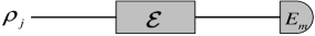
Figure 1: Schematic of SQPT. An ensemble of states $\{\rho_{j}\}$ are prepared and each of them is subjected to the map $\mathcal{E}$, and then to the measurements $\{E_{m}\}$.

The central idea of SQPT is to prepare $d^{2}$ linearly-independent inputs $\{\rho_{k}\}_{k=0}^{d^{2}-1}$ and then measure the output states $\mathcal{E}(\rho_{k})$ by using quantum state tomography nielsen-book ; chuang-sqpt ; poyatos-sqpt . SQPT has been experimentally demonstrated in liquid-state NMR childs-nmr ; boulant-lindblad ; weinstein-qpt , optical steinberg-bell ; obrien-cnot , atomic steinberg-qpt2 and solid-state systems howard . Since the map $\mathcal{E}$ is linear, it can in principle be reconstructed from the measured data by a proper inversion. Let $\{\rho_{k}\}_{k=0}^{d^{2}-1}$ be a linearly independent basis set of operators for the space of $d\times d$ linear operators. A convenient choice is $\rho_{k}=|m\rangle\langle n|$, where $\{|m\rangle\}_{m=0}^{d-1}$ is an orthonormal basis for $\mathcal{H}$. The coherence $|m\rangle\langle n|$ can be reconstructed from four populations: $|m\rangle\langle n|=|+\rangle\langle+|+|-\rangle\langle-|-[|m\rangle\langle m|+|n\rangle\langle n|](1+i)/2$, where $|+\rangle=(|m\rangle+|n\rangle)/\sqrt{2}$ and $|-\rangle=(|m\rangle+i|n\rangle)/\sqrt{2}$. Linearity of $\mathcal{E}$ then implies that measurement of $\mathcal{E}(|+\rangle\langle+|)$, $\mathcal{E}(|-\rangle\langle-|)$, $\mathcal{E}(|m\rangle\langle m|)$, and $\mathcal{E}(|n\rangle\langle n|)$ suffices for the determination of $\mathcal{E}(|m\rangle\langle n|)$. In addition, every $\mathcal{E}(\rho_{k})$ can be expressed in terms of a linear combination of basis states, as $\mathcal{E}(\rho_{k})=\sum_{l}\lambda_{kl}\rho_{l}$. The parameters $\lambda_{kl}$ contain the measurement results, and can be understood as the expectation values of the fixed-basis operators $E_{k}\text{: }$

$$\lambda_{kl}=\text{Tr}(E_{k}\mathcal{E}(\rho_{l})),$$ (4)

when $E_{k}=\rho_{k}$. This choice of the $E_{k}$ is natural, since the $\rho_{k}$ are Hermitian operators and thus they are valid observables. If we combine this with the relation $E_{m}\rho_{k}E_{n}^{\dagger}=\sum_{l}B_{mn,lk}\rho_{l}$, the following equation can be obtained: $\sum_{mn}B_{mn,lk}\chi_{mn}=\lambda_{kl}$. This in turn can be written in the following matrix form:

$$\bm{B}\bm{\chi}=\bm{\lambda},$$ (5)

where the $d^{4}\times d^{4}$-dimensional matrix $\bm{B}$ is determined by the choice of bases $\{\rho_{k}\}$ and $\{E_{m}\}$, and the $d^{4}$-dimensional vector $\bm{\lambda}$ is determined from the state tomography experiments. The superoperator $\bm{\chi}$ can thus be determined by inversion of Eq. (5), but in general $\bm{\chi}$ is not uniquely determined by this equation.

Figure 1 illustrates the SQPT scheme. Let us determine the resources this scheme requires. In general, SQPT involves preparation of $d^{2}$ linearly independent inputs $\{\rho_{l}\}$, each of which is subjected to the quantum process $\mathcal{E}$, followed by quantum state tomography on the corresponding outputs. As we saw above, for each $\rho_{l}$ we must measure the expectation values of the $d^{2}$ fixed-basis operators $\{E_{k}\}$ in the state $\mathcal{E}(\rho_{l})$. Thus the total number of required measurements amounts to $d^{4}$. Since measurement of an expectation value cannot be done on a single copy of a system, throughout this paper, whenever we use the term “measurement” we implicitly mean measurement on an ensemble of identically prepared quantum systems corresponding to a given experimental setting.

IV Ancilla-Assisted Process Tomography

In principle, there is an intrinsic analogy between quantum state tomography schemes and QPT. This analogy is based upon the well-known Choi-Jamiolkowski isomorphism choi-jamilolkowksi , which establishes a correspondence between completely-positive quantum maps (or operations) and quantum states, $\mathcal{E}\rightarrow\rho_{\mathcal{E}}$, as follows:

$$\rho_{\mathcal{E}}\equiv(\mathcal{E}\otimes I)(|\Phi^{+}\rangle\langle\Phi^{+}|),$$ (6)

where $|\Phi^{+}\rangle=\sum_{i=1}^{d}\frac{1}{\sqrt{d}}|i\rangle\otimes|i\rangle$ is the maximally entangled state of the system and an ancilla with the same size. This one-to-one map enables all of the theorems about quantum operations directly to be derived from those of quantum states arrighi . In this way, one can consider a quantum process as a quantum state (in a larger Hilbert space). Therefore, the identification of the original map $\mathcal{E}$ is equivalent to the characterization of the corresponding state $\rho_{\mathcal{E}}$. In other words, the problem of quantum process tomography can naturally be reduced to the problem of quantum state tomography, and hence, all state identification techniques can be applied to the characterization of quantum processes as well. The AAPT scheme was built exactly upon this basis.

Generally, within the AAPT scheme, we attach an auxiliary system (ancilla), $B$, to our principal system, $A$, and prepare the combined system in a single state such that complete information about the dynamics can be imprinted on the final state d'ariano-aapt ; altepeter-aapt . Then by performing quantum state tomography in the extended Hilbert space of $\mathcal{H}_{AB}$, one can extract complete information about the unknown map acting on the principal system. In principle, the input state of the system and ancilla can be prepared in either an entangled mixed state (entanglement-assisted) or a separable mixed state. Intuitively, the input state in AAPT must be faithful enough to the map $\mathcal{E}$ such that by quantum state tomography on the outputs one can identify $\mathcal{E}$ completely and unambiguously d'ariano-faithful . This faithfulness condition can formalized. Indeed, it is easy to show that a state $\rho$ can be used as input for AAPT iff $\rho$ has maximal Schmidt number, i.e. $\text{Sch}(\rho)=d^{2}$ altepeter-aapt . The faithfulness condition is nothing but an invertibility condition. That is, because of linearity of the map $\mathcal{E}\otimes I,$ the information is imprinted on the elements of the final output states linearly. By performing state tomography on the output state $(\mathcal{E}\otimes I)(\rho)$, we obtain a set of linear relations among possible measurement outcomes and the elements of $\mathcal{E}$ and $\rho$. The matrix $\rho$ must be chosen such that an inversion becomes possible; thus one can solve the set of linear equations for $\mathcal{E}$ d'ariano-aapt . We provide more details below.

It should be noted that the faithfulness condition is different from entanglement. In fact, almost all states of the combined system $AB$ (excluding product states) may be used for AAPT, because the set of states with Schmidt number less than $d^{2}$ is of zero measure. This means that entanglement is not a necessary property of the input state $\rho$ in AAPT. Indeed, many of the viable input states are not entangled, such as Werner states altepeter-aapt . However, it has been argued and also experimentally verified that use of maximally entangled pure states offers the best performance. That is, even though in principle any faithful state can be used in AAPT, the propagation of experimental errors from the measurement outcomes to actual estimation of $(\mathcal{E}\otimes I)(\rho)$, due to the inversion process, dictates that different faithful input states can produce very different errors.

In order to develop a good faithfulness measure, one can consider a general property of a typical input state $\rho$, such that the output states generated by different quantum dynamical processes have maximum distance; e.g., different output states should be nearly orthogonal. More specifically, we note that the experimental error amplification is related to the inversion, which in turn depends on the multiplication by the inverse of the eigenvalues of $\rho$, $s_{l}^{-1}$. Then, the smaller the eigenvalues the higher the amplification of experimental errors. This fact has led to the following definition:

$$F(\rho)=\text{Tr}(\rho^{2})=\sum_{l=1}^{d^{2}}s_{l}^{2},$$

as a proper measure of faithfulness d'ariano-aapt . This, indeed, is exactly the purity of the state $\rho$. As a consequence, this implies that the optimal (in the sense of minimal experimental errors, as explained above) faithful input states are pure states with maximal Schmidt number and $s_{l}=1/\sqrt{d}$, i.e., maximally entangled pure states.

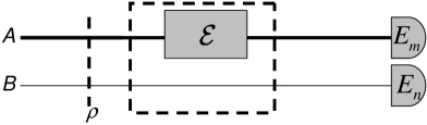
Figure 2: Schematic diagram of separable AAPT. An ensemble of systems is prepared in the same quantum state $\rho$. Next, they are subjected to the map $\mathcal{E}\otimes I$. Finally the operators $\{E_{j}\}$ are measured on both the system and the ancilla, which results in the required joint probability distributions or expectation values.

The Hilbert space of the input state in AAPT is $\mathcal{H}_{AB}\equiv\mathcal{H}_{A}{\otimes}\mathcal{H}_{B}$. At the output, one can realize the required quantum state tomography by either separable measurements (separable AAPT), i.e., joint measurement of tensor product operators, or collective measurements on both the system and ancilla (non-separable AAPT). Both of these measurements are performed on the same Hilbert space $\mathcal{H}_{AB}$. Furthermore, it is possible to perform a generalized measurement or POVM by going to a larger Hilbert space. In the subsequent sections, we discuss all of these alternative strategies and argue that the non-separable measurement schemes (whether in the same Hilbert space or in a larger one) have hardly any practical relevance in the context of QPT, because they require many-body interactions which are experimentally unavailable.

IV.1 Joint separable measurements

Let us assume that the initial state of the system and ancilla is $\rho_{AB}=\sum_{ij}\rho_{ij}E_{i}^{A}\otimes E_{j}^{B}$, where $\{E_{m}^{A}\}$ ($\{E_{n}^{B}\}$) is the operator basis for the linear operators acting on $\mathcal{H}_{A}$ ($\mathcal{H}_{B}$), as defined earlier. The output state, after applying the unknown map $\mathcal{E}$ on the principal system, is the following:

$$\rho_{AB}^{\prime} = (\mathcal{E}_{A}\otimes I_{B})(\rho_{AB})$$ (7)

$$= \sum_{ij,mn}\rho_{ij}\chi_{mn}E_{m}^{A}E_{i}^{A}E_{n}^{A\dagger}\otimes E_{j}^{B}$$

$$= \sum_{kj}\tilde{\alpha}_{kj}E_{k}^{A}\otimes E_{j}^{B}.$$

In the last line, we have used $\tilde{\alpha}_{kj}=\sum_{mni}\chi_{mn}\rho_{ij}\alpha_{k}^{m,i,n}$, where $\alpha_{k}^{m,i,n}$ is defined via $E_{m}^{A}E_{i}^{A}E_{n}^{A\dagger}=\sum_{k}\alpha_{k}^{m,i,n}E_{k}^{A}$, and depends only on the choice of operator basis. From the above equation it is clear that if we consider the basis operators as observables, then the parameters $\widetilde{\alpha}_{kj}$, which are related to the $\chi_{mn}$’s, can be obtained by joint measurement of the observables $E_{k}^{A}\otimes E_{j}^{B}$. In fact, the expectation values $\text{Tr}(\rho_{AB}^{\prime}E_{k}^{A\dagger}\otimes E_{j}^{B\dagger})$, as the measurement results, are exactly the $\widetilde{\alpha}_{kj}$ parameters:

$$\widetilde{\alpha}_{kj}=\text{Tr}(\rho_{AB}^{\prime}E_{k}^{A\dagger}\otimes E_{j}^{B\dagger}).$$ (8)

Now, by defining

$$\widetilde{\chi}_{ki}=\sum_{mn}\alpha_{k}^{m,i,n}\chi_{mn},$$ (9)

and considering that the $\alpha$ parameters are known from the choice of operator basis, we see that by knowledge of the $\widetilde{\alpha}_{kj}$’s we can obtain the $\chi_{mn}$ parameters through the following matrix equation:

$$\widetilde{\bm{\alpha}}=\widetilde{\bm{\chi}}~{}\bm{\varrho},$$ (10)

where $\bm{\varrho}=[\rho_{ij}]$, $\widetilde{\bm{\chi}}=[\widetilde{\chi}_{mn}]$, and $\widetilde{\bm{\alpha}}=[\widetilde{\alpha}_{kl}]$. This equation implies that unambiguous and unique determination of the $\widetilde{\bm{\chi}}$ matrix is possible iff the $\bm{\varrho}$ matrix is invertible. After obtaining $\widetilde{\bm{\chi}}$, by using the linear relation of Eq. (9) between $\widetilde{\bm{\chi}}$ and $\bm{\chi}$ matrices, one can easily find $\bm{\chi}$ by an inversion.

Equation (10) implies that if we were to choose $\bm{\varrho}$ as a multiple of the $d^{2}\times d^{2}$ identity matrix $I$, then the unknown quantum operation, $\widetilde{\bm{\chi}}$, would be directly related to the measurement results, $\widetilde{\bm{\alpha}}$, without the need for inversion. However, positivity of the density matrix $\rho_{AB}$ disallows this choice. For example, in the qubit case, it can be easily seen that the operators $\bm{\varrho}=\frac{1}{2}~{}I$ results in $\rho_{AB}=\frac{1}{4}(I_{A}\otimes I_{B}+X_{A}\otimes X_{B}+Y_{A}\otimes Y_{B}+Z_{A}\otimes Z_{B})$, which is physically unacceptable because of its negativity. Conversely, Eq. (10) implies that in AAPT no choice of the initial density matrix $\rho_{AB}$ can result in a direct (inversion-free) relation between the measurement results and elements of the unknown map.

Next, we explicitly show that the invertibility condition of $\bm{\varrho}$ in Eq. (10) is equivalent to the condition of maximal Schmidt number in the corresponding $\rho_{AB}$. In general, an operator $Q_{AB}$ on $\mathcal{H}_{A}\otimes\mathcal{H}_{B}$ can be written as $Q=\sum_{jk}Q_{jk}C_{j}\otimes D_{k}$, where $\{C_{j}\}$ ($\{D_{k}\}$) is a fixed orthonormal basis for the space of linear operators acting on $\mathcal{H}_{A}$ ($\mathcal{H}_{B}$). A singular value decomposition of the matrix $\bm{Q}\equiv[Q_{jk}]$ yields $\bm{Q}=USV$, where $U$ and $V$ are unitary matrices and $S$ is a diagonal matrix with non-negative entries $S_{jk}=s_{k}\delta_{jk}$ ($s_{k}$ are the singular values of the matrix $\bm{Q}$). Using this decomposition, we have $Q=\sum_{l}s_{l}A_{l}\otimes B_{l}$, where the operators $\{A_{l}\equiv\sum_{j}U_{jl}C_{j}\}$ and $\{B_{l}\equiv\sum_{k}V_{lk}D_{k}\}$ are also orthonormal bases. This is the Schmidt decomposition of the operator $Q$ nielsen-dynamics . In our case, $\bm{Q}$ is the matrix $\bm{\varrho}$. We know that $\bm{\varrho}$ is invertible iff none of its singular values is zero, i.e. $\forall l,s_{l}\neq 0$. This, in turn, guarantees that in the Schmidt decomposition of $\rho_{AB}$ (counterpart of $Q$) all terms are present, that is, it has maximal Schmidt number. This confirms that the invertibility condition—which is necessary for the applicability of input states in AAPT—is exactly what was already termed faithfulness above (for more detail see Ref. MasoudThesis ). In fact, even separable Werner states, $\rho_{\epsilon}=\frac{1-\epsilon}{d^{2}}I+\epsilon|\Psi^{-}\rangle\langle\Psi^{-}|$ (in which $|\Phi^{-}\rangle_{AB}=(|01\rangle-|10\rangle)_{AB}/\sqrt{2}$) for $\epsilon\leqslant\frac{1}{1+d}$ braunstein-nmr , have maximal Schmidt number. Therefore even classical correlation between the system and the ancilla is sufficient for AAPT.

IV.2 Mutually unbiased bases measurements

Ancilla-assisted quantum process tomography can also be performed by using “mutually unbiased bases” (MUB) measurements ivanovic-mub ; wootters-mub . Let us briefly review MUB, their properties, and physical importance in the context of quantum measurement.

Assume that $\{|a_{i}\rangle\}_{i=0}^{d-1}$ and $\{|b_{i}\rangle\}_{i=0}^{d-1}$ are two different basis sets for the $d$-dimensional Hilbert space $\mathcal{H}$. They are called mutually unbiased if they fulfill the following condition:

$$|\langle a_{i}|b_{j}\rangle|^{2}=\frac{1}{d}~{}\forall i,j.$$

As an example, for $d=2$ (the case of a single qubit) it is easy to verify that the eigenvectors of the three Pauli matrices, $X$, $Y$, $Z$, denoted respectively by $\{|\pm\rangle\}_{X}$, $\{|\pm\rangle\}_{Y}$, and $\{|0\rangle,|1\rangle\}$, constitute a set of pairwise MUB. In general, the maximum number of MUB for an arbitrary dimensional vector space is not yet known, however, it has been proved that it cannot be greater than $d+1$. In addition, for $d$ being a power of prime, it has been proved that the number of MUB is exactly $d+1$ and explicit construction algorithms are already known som-mub ; wootters-mub .

Table 1: A partitioning of the 2-qubit Pauli group such that the eigenvectors constitute a MUB.

MUB 1	$Z^{A}$	$Z^{B}$	$Z^{A}Z^{B}$
MUB 2	$X^{A}$	$X^{B}$	$X^{A}X^{B}$
MUB 3	$Y^{A}$	$Y^{B}$	$Y^{A}Y^{B}$
MUB 4	$X^{A}Z^{B}$	$Y^{A}X^{B}$	$Z^{A}Y^{B}$
MUB 5	$X^{A}Y^{B}$	$Y^{A}Z^{B}$	$Z^{A}X^{B}$

For the case of $n$-qubit systems ($d=2^{n}$) one can show the set of $4^{n}-1$ Pauli operators, $\tilde{E}_{k}\equiv\otimes_{i=1}^{n}E_{\alpha(i,k)}^{i}$, where $E_{\alpha}\in\{I,X,Y,Z\}$, can be partitioned into $2^{n}+1$ distinct subsets, each consisting of $2^{n}-1$ mutually commuting observables. All the operators in each subset have a set of joint eigenvectors. The eigenvectors of all subsets then form MUB lawrence-mub ; Romero-mub . Table 1 illustrates such a MUB based partitioning of the 2-qubit Pauli operators.

The importance of MUB which is relevant to our discussion is their application in quantum state estimation. To determine the density matrix of a $d$-dimensional quantum system $d^{2}-1$ independent real parameters must be determined. The most informative (sub)ensemble measurements of an observable $\Omega$ of the system (whose spectrum is non-degenerate) provide $d-1$ independent data points, namely the probabilities $\text{Tr}(\rho\pi_{i})$, where $\Omega=\sum_{i}\omega_{i}\pi_{i}$ is the spectral decomposition of $\Omega$ with spectrum $\omega_{i}$. Thus, to fully determine the density matrix we must measure at least $(d^{2}-1)/(d-1)=d+1$ different noncommuting observables. In this sense measurement of the observables corresponding to MUB is optimal, because this requires the smallest possible number of noncommuting measurements. Moreover, due to the finiteness of ensembles any repeated measurement will give rise to statistical errors. Naturally, to reduce such errors one must increase the size of ensembles and then repeat the measurements. However, it has been shown that a set of $d+1$ MUB measurements provides the optimal estimation of an unknown quantum state, i.e., generates minimal statistical error (if such MUB exist) wootters-mub .

Now, we demonstrate that MUB measurements for state tomography yields another version of AAPT. Let us first specialize to the single qubit case. As noted earlier, to determine a general quantum dynamical map on a single qubit using AAPT, one attaches an ancilla and performs quantum state tomography at the end. In this case, the dimension of the combined Hilbert space is $d=2^{2}$ (we assume that the dimension of the ancilla is the same as that of the system). It follows from the general arguments above that one can use $d+1=5$ MUB measurements to determine the final state of the combined system (see Fig. 3). These measurements are in fact optimal in the sense explained earlier. The first (as always, ensemble) measurement provides four independent outcomes and each of the remaining ones yields three independent results, which totals, as required, $4+(4\times 3)=16$ results.

It should be noted that even if the local state of the ancilla is known (i.e., if we know the expectation values of $I^{A}\otimes I^{B}$, $I^{A}\otimes X^{B}$, $I^{A}\otimes Y^{B}$ and $I^{A}\otimes Z^{B}$ from prior knowledge about the preparation and trace-preserving property of the quantum map), the number of required measurements is still five ziman-note ; mohseni-reply . This can easily be seen from Table 1. For a non trace-preserving map we need five measurements of the (commuting) operators of the first and the second columns (the elements of the third column are products of the operators in the first two columns). If we know the local state of the ancilla $B$, the first three measurements of the second column are redundant. However, since the operators in the first column do not commute we still need to perform three (ensemble) measurements corresponding to the first three rows. The remaining two measurements related to the fourth and fifth rows are also necessary and they correspond to measuring the correlations of the principal qubit and the ancilla. Thus, the overall number of required MUB measurements in the case of trace-preserving maps is still $5$. This argument is independent of the basis chosen, because in any other basis, due to noncommutativity of the Pauli operators, the measurements corresponding to the local state of the ancilla always appear in different rows.

For the case of $n$-qubit AAPT, the dimension of the joint system-ancilla Hilbert space is $d=2^{2n}$. In this Hilbert space four different strategies can be devised: (i) using $16^{n}$ (separable) joint single-qubit measurements on the $n$-qubit system and the $n$-qubit ancilla (as explained earlier—Fig. 2), (ii) using $5^{n}$ MUB based measurements (tensor products of MUB based measurements of two-qubit systems), (iii) using $d+1=4^{n}+1$ MUB based measurements on all $2n$ qubits, or (iv) using different combinations of single-, two-, and multi-qubit measurements including MUB based measurements (the number of measurements ranges from $4^{n}+1$ to $16^{n}$). In what follows, we focus on method (iii) because it is the most economical in terms of the total number of measurements.

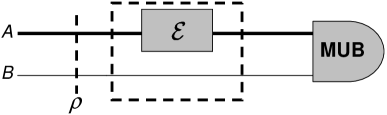
Figure 3: Schematic diagram of non-separable AAPT. In this scheme the joint separable measurements of Fig. 2 have been replaced by (collective) mutually unbiased bases measurements on the two systems.

The main drawback of performing a MUB based measurement on all $2n$ qubits is that it requires many-body interactions between all $2n$ qubits. From an experimental point of view, such many-body interactions are not naturally available. This does not mean that they cannot be simulated, but as we will see this comes at a high resource cost. This is a strong restriction which seriously affects the advantage of method (iii). According to our earlier discussion, the general multi-qubit observables in a MUB based measurement are generated from $2^{2n}+1$ noncommuting classes (or partitions) of $2n$-qubit operators $\{[\tilde{E}_{1}],\ldots,[\tilde{E}_{2^{2n}+1}]\}$, where each class $[\tilde{E}_{k}]$ contains $2^{2n}-1$ commuting observables, and $\tilde{E}_{k}\equiv\otimes_{i=1}^{n}E_{\alpha(i,k)}^{i}$ with $E_{\alpha}^{i}\in\{I,X^{i},Y^{i},Z^{i}\}$ (for the case of three qubits refer to Fig. 2 of Ref. lawrence-mub ).

In principle, one can simulate such many-body interactions from single- and two-qubit gates (e.g., CNOT). We next argue that the complexity of such a quantum simulation scales at least as $\mathcal{O}(n^{2})$ or $\mathcal{O}(n^{3})$ depending, respectively, on the availability of non-local or local MUB measurements.

All operators $\tilde{E}_{m}$ and $\tilde{E}_{n}$ that belong to the same class $[\tilde{E}_{k}]$ commute and are composed of tensor products of identity and/or Pauli operators. However, they cannot be simultaneously measured locally, i.e. by using only single-qubit observables. The reason is that each local measurement $E_{\alpha(i,m)}^{i}$ for the operator $\tilde{E}_{m}$ completely destroys the outcome of measuring $E_{\alpha(i,n)}^{i}$ for the other operator $\tilde{E}_{n}$, due to noncommutativity of the Pauli operators. It is simple to see that for the non-separable measurement of an operator such as $Z^{1}Z^{2}\ldots Z^{2n}$, we need $2n$ sequential CNOT gates. To measure a more general observable such as $\tilde{E}_{k}\equiv\ E_{\alpha_{1}}^{1}\ldots E_{\alpha_{2n}}^{2n}$, where $E_{\alpha_{i}}^{i}\in\{I,X^{i},Y^{i},Z^{i}\}$, we need $\mathcal{O}(n)$ additional single-qubit rotations to make appropriate basis changes. Therefore, for measuring $n$ such general operators from the class $[\tilde{E}_{k}]$, one needs to realize $\mathcal{O}(n^{2})$ basic quantum operations. The condition for such a construction is the possibility of addressing arbitrary distant pairs of qubits (i.e., having access to non-local two-body interactions). This is an important point, because in practical realizations the spatial arrangements of the qubits or other technological reasons may limit the interactions between distant qubits. If only nearest neighbor gates can be implemented then pairs of qubits must be brought close to one another (e.g., via swap gates), which incurs a cost of $\mathcal{O}(n)$ operations per pair mottonen-gates . In this case, we need $\mathcal{O}(n^{3})$ quantum gates to simulate the required multi-qubit measurements. It should also be noted that in such a simulation the scaling of execution time and possible (operational) errors in the measurements will introduce additional experimental complications.

IV.3 Generalized measurement

In principle, it is also possible to perform the required quantum state tomography at the output of AAPT by utilizing only a single generalized measurement or POVM d'ariano-universal ; d'ariano-EuroPhys . Suppose that we want to determine an unknown state $\rho$ of our quantum system. In a $d$-dimensional Hilbert space characterization of $\rho$ requires determination of $d^{2}-1$ independent real parameters. In order to design a scheme for determination of $\rho$ by a single quantum observable, we need to attach a $d^{\prime}$-dimensional ancilla ($B$) with a known initial state $r$ to our principal system ($A$). In the scheme proposed in Ref. d'ariano-universal , one should measure one of the observables of the combined system ($AB$), a “universal quantum observable”,

$$\Omega=\sum_{a=1}^{dd^{\prime}}\lambda_{a}P_{a},$$ (11)

where $\Omega$ is a normal operator and the spectrum $\lambda_{a}$ should be non-degenerate such that the projections $P_{a}$ constitute a complete set of $dd^{\prime}-1$ commuting observables. Since the projections all commute, one can measure all of them simultaneously using a single apparatus. Such (repeated ensemble) measurements provide us with $dd^{\prime}-1$ probabilities $p_{a}=\text{Tr}(P_{a}\rho\otimes r)$. The dimension of the ancilla must be greater than or equal to the dimension of the system, $d^{\prime}\geqslant d$. If we take $\rho=\sum_{nm}\rho_{nm}|n\rangle\langle m|$ and $r=\sum_{\alpha\beta}r_{\alpha\beta}|\alpha\rangle\langle\beta|$, then we obtain the following linear relation:

$$\rho\mapsto p_{a}=\sum_{mn}M_{mn}^{a}\rho_{nm},$$ (12)

where $M_{mn}^{a}=\sum_{\alpha\beta}r_{\alpha\beta}\langle m\beta|P_{a}|n\alpha\rangle$. When $d=d^{\prime}$ and the measured observable $\Omega$ couples $A$ and $B$ in a manner such that $\bm{M}_{a,mn}\equiv M_{mn}^{a}$ is invertible ($\text{det}\bm{M}\neq 0$), a linear inversion can reveal the unknown state $\rho$ alla .

To be specific, we choose $\Omega$ as follows:

$$\Omega=\sum_{a=1}^{d^{2}}aE_{a}^{A}\otimes E_{a}^{B},$$ (13)

where $\{E_{a}^{A}\}_{a=1}^{d^{2}}$ ($\{E_{a}^{B}\}_{a=1}^{d^{2}}$) is a set of orthonormal basis operators for the space of linear operators on $\mathcal{H}_{A}$ ($\mathcal{H}_{B}$). Using the representation $T=\sum_{a}\mathrm{Tr}(TE_{a}^{{\dagger}})E_{a}$ (for any operator $T$), it is not hard to see that the ensemble average of an arbitrary operator $O$ (on $\mathcal{H}_{A}$) is equivalent to an ensemble average of the following function of $\Omega$:

$$F_{O}(\Omega)=\sum_{a}\frac{\text{Tr}(OE_{a}^{A\dagger})}{\text{Tr}(rE_{a}^{B})}E_{a}^{A}\otimes E_{a}^{B},$$

on $\rho\otimes r$, i.e.,

$$\langle O\rangle_{\rho}=\langle F_{O}(\Omega)\rangle_{\rho\otimes r}.$$ (14)

Therefore estimation of the ensemble average $\langle O\rangle_{\rho}$ of an operator $O$ acting on the principal system $A$, can be achieved by measuring $F_{O}(\Omega)$ on the joint $A$ and $B$ system. This allows for the estimation of every ensemble average for the principal quantum system.

The above general scheme can also be utilized for quantum process tomography (Fig. 3 in Ref. d'ariano-universal ). It is sufficient to consider the AAPT scheme and attach two additional ancillas (one for the system and another for the ancilla of the AAPT scheme), and then measure jointly two universal observables (Fig. 4). In this manner, to characterize the dynamics of $n$ qubits, the number of required ancillary qubits increases from $n$ (in AAPT) to at least $3n$. This can be easily understood via a simple counting argument. In order to extract complete information about a quantum dynamical map on $n$ qubits (encoded by $2^{4n}$ independent parameters of the superoperator $\bm{\chi}$) in a single measurement, one needs a Hilbert space of dimension at least $2^{4n}$ on which the information can be imprinted unambiguously.

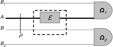
Figure 4: Schematic diagram of a QPT by using POVM. Here we have used the idea of “universal quantum observable” d'ariano-universal . To accomplish complete process tomography, one needs two more ancillas $B_{1}$ and $B_{2}$ (in addition to the one used in AAPT, $B$) and two universal quantum observable $\Omega_{1}$ and $\Omega_{2}$.

There are two major disadvantages in using such a POVM compared to all other QPT schemes. First, the POVM scheme requires a general many-body interaction between all $2n$ qubits that are measured through each $\Omega_{i}$. This interaction cannot be efficiently simulated, i.e., it requires an exponential number of elementary single- and two-qubit quantum gates. Indeed, the above universal quantum observable scheme is very difficult to implement in practice, because it implies measuring an observable $\Omega$ (or a commuting set $\{P_{a}\}$) which thoroughly entangles the system and the ancilla(s). There is an alternative method to implement the above scheme alla , by interacting system and ancilla for a specific time duration $\tau$ through a known unitary operator $U$ (or known Hamiltonian $H$), and then measuring the simplest possible non-degenerate observable $\Omega$, namely a factorized quantity $\Omega=\omega^{A}\otimes\omega^{B}$ d'ariano-universal ; alla . However, even this method still requires a many-body interaction (through $U$) which is difficult to prepare. The operator $\Omega$ has maximal Schmidt number and generally cannot be simulated using a polynomial number of elementary gates. It is known that, in general, $\mathcal{O}(4^{N})$ elementary single- and two-qubit gates are necessary to simulate many-body operations acting on $N$ qubits shende (see also Ref. nielsen-dynamics for different measures of complexity of a given quantum dynamics, and Ref. jozsa-entcost for the concept of entanglement cost of a POVM).

V Direct Characterization of Quantum Dynamics

Recently a new scheme for quantum process identification was proposed and termed “direct characterization of quantum dynamics” (DCQD) mohseni-dcqd1 ; mohseni-dcqd2 . It differs in a number of essential aspects from SQPT and AAPT. In DCQD, similarly to AAPT, the degrees of freedom of an ancilla system are utilized, but in contrast it does not require inversion of a full $d^{2}\times d^{2}$ matrix (hence “direct”); it requires different input states; and uses a fixed measurement apparatus (Bell state analyzer) at the output. The main idea in DCQD is to use certain entangled states as inputs and to perform a simple error-detecting measurement on the joint system-ancilla Hilbert space. A combination of these input states and measurements give rise to a direct encoding of the elements of the quantum map into the measurement results, which removes the need for state tomography. More precisely, by “direct” we mean that the measured probability distributions (on an ensemble of the setting) are rather directly related, i.e., without the need for a complete inversion, to the elements of $\bm{\chi}$. In essence, in DCQD the $\bm{\chi}$ matrix elements of linear quantum maps become directly experimentally observable. For the case of single qubit, the measurement scheme turns out to be equivalent to a Bell-state measurement (BSM). In DCQD the choice of input states is dictated by whether diagonal (population) or off-diagonal (coherence) elements of the superoperator are to be determined. Population characterization requires maximally entangled input states, while coherence characterization requires non-maximally entangled input states. In the following, we review the scheme for the case of qubits. For a generalization of the scheme to higher-dimensional quantum systems see Ref. mohseni-dcqd2 .

Let us consider the case of a single qubit and demonstrate how to determine all diagonal elements of the superoperator, $\{\chi_{mm}\}$, in a single (ensemble) measurement. We choose $\{I,X^{A},Y^{A},Z^{A}\}$ as our error operator basis acting on the principal qubit $A$. We first maximally entangle the two qubits $A$ (the principal system) and $B$ (the ancilla) in a Bell-state $|\Phi^{+}\rangle=(|00\rangle+|11\rangle)_{AB}/\sqrt{2}$ (an instance of a stabilizer code), and then subject only qubit $A$ to the map $\mathcal{E}$.

A stabilizer code is a subspace $\mathcal{H}_{C}$ of the Hilbert space of $n$ qubits that is an eigenspace of a given Abelian subgroup $\mathcal{S}$ (the stabilizer group) of the $n$-qubit Pauli group, with eigenvalue $+1$ nielsen-book ; gottesman-thesis . In other words, for every $|\Psi_{C}\rangle\in\mathcal{H}_{C}$ and all $S_{i}\in\mathcal{S}$, we have $S_{i}|\Psi_{C}\rangle=|\Psi_{C}\rangle$, where the $S_{i}$’s are the stabilizer generators and $[S_{i},S_{j}]=0$ for all $i$ and $j$. Consider the action of an arbitrary error operator $E$ on the stabilizer code state: $E|\Psi_{C}\rangle$. The detection of such an error will be possible if the error operator anticommutes with (at least one of) the stabilizer generators: $\{S_{i},E\}=0$. To see this note that

$$S_{i}(E|\Psi_{C}\rangle)=-E(S_{i}|\Psi_{C}\rangle)=-(E|\Psi_{C}\rangle),$$

i.e., $E|\Psi_{C}\rangle$ is a $-1$ eigenstate of $S_{i}$. Hence measurement of $S_{i}$ detects the occurrence of an error or no error ($-1$ or $+1$ outcomes, respectively). Measuring all the generators of the stabilizer then yields a list of errors (“syndrome”), which allows one to determine the nature of the errors unambiguously.

The state $|\Phi^{+}\rangle$ is a $+1$ eigenstate of the commuting operators $Z^{A}Z^{B}$ and $X^{A}X^{B}$, i.e., it is stabilized under the action of these stabilizer generators. It is easy to see that any non-trivial error operator $E_{i}\in\{I,X^{A},Y^{A},Z^{A}\}$ acting on the state of the qubit $A$ anticommutes with at least one of the stabilizer generators, and therefore by measuring them simultaneously we can detect the error:

$$\begin{array}[]{c}X^{A}X^{B}\\ Z^{A}Z^{B}\end{array}(E_{i}^{A}|\Phi^{+}\rangle)=\pm(E_{i}^{A}|\Phi^{+}\rangle).$$

Note that measuring the observables $Z^{A}Z^{B}$ and $X^{A}X^{B}$ is indeed equivalent to a BSM, and can be represented by the four projection operators $P_{\Psi^{\pm}}=|\Psi^{\pm}\rangle\left\langle\Psi^{\pm}\right|$ and $P_{\Phi^{\pm}}=|\Phi^{\pm}\rangle\langle\Phi^{\pm}|$, where $|\Phi^{\pm}\rangle=(|00\rangle\pm|11\rangle)/\sqrt{2}$ , and $|\Psi^{\pm}\rangle=(|01\rangle\pm|10\rangle)/\sqrt{2}$ are the Bell states. The probabilities of obtaining the no-error outcome $I$, bit-flip error $X^{A}$, phase-flip error $Z^{A}$, and both phase-flip and bit-flip errors $Y^{A}$, on qubit $A$ can be expressed as:

$$p_{m}=\text{Tr}[P_{m}\mathcal{E}(\rho)]=\chi_{mm},$$ (15)

where $m=0,1,2,3$, and the projectors $P_{m}$, for $m=0,1,2,3$, correspond to the states $\Phi^{+}$, $\Psi^{+}$, $\Psi^{-}$, and $\Phi^{-}$, respectively. Here $\mathcal{E}(\rho)$ is a shorthand for $(\mathcal{E}\otimes I)(\rho)$. Equation (15) is a remarkable result: it shows that the diagonal elements of the superoperator are directly obtainable from an ensemble BSM. This is the core observation that leads to the DCQD scheme. In particular, we can determine the quantum dynamical populations, $\chi_{mm}$, in a single ensemble measurement (i.e., by simultaneously measuring the operators $Z^{A}Z^{B}$ and $X^{A}X^{B}$) on multiple copies of the state $|\Phi^{+}\rangle$).

To determine the coherence elements, $\chi_{m\neq n}$, a modified strategy is needed. As the input state we take a non-maximally entangled state: $|\Phi_{\alpha}^{+}\rangle=\alpha|00\rangle+\beta|11\rangle$, with $|\alpha|,|\beta|\notin\{0,1/\sqrt{2}\}$ and $\text{Im}(\alpha\bar{\beta})\neq 0$. The sole stabilizer of this state is $Z^{A}Z^{B}$. The spectral decomposition of this stabilizer is $Z^{A}Z^{B}=P_{+1}-P_{-1}$, where $P_{\pm 1}$ are projection operators defined as $P_{+1}=P_{\Phi^{+}}+P_{\Phi^{-}}$ and $P_{-1}=P_{\Psi^{+}}+P_{\Psi^{-}}$. Now, it is easy to see that by measuring $Z^{A}Z^{B}$ on the output state $\mathcal{E}(\rho)$, with $\rho=|\Phi_{\alpha}^{+}\rangle\langle\Phi_{\alpha}^{+}|$, we obtain:

$$\text{Tr}[P_{+1}\mathcal{E}(\rho)]=\chi_{00}+\chi_{33}+2\mathrm{Re}(\chi_{03})\langle Z^{A}\rangle,$$ (16)

and

$$\text{Tr}[P_{-1}\mathcal{E}(\rho)]=\chi_{11}+\chi_{22}+2\mathrm{Im}(\chi_{12})\langle Z^{A}\rangle,$$ (17)

where $\langle Z^{A}\rangle=\text{Tr}(\rho Z^{A})\neq 0$ because of our choice of a non-maximally entangled input state ($|\alpha|,|\beta|\notin\{0,1/\sqrt{2}\}$). The experimental data, Tr$[P_{\pm 1}\mathcal{E}(\rho)]$, are exactly the probabilities of no bit-flip error and a bit-flip error on qubit $A$, respectively. Since we already know the $\chi_{mm}$’s from the population measurement, we can determine $\mathrm{Re}(\chi_{03})$ and $\mathrm{Im}(\chi_{12})$. After measuring $Z^{A}Z^{B}$ the system is in either of the states $\rho_{\pm 1}=P_{\pm 1}\mathcal{E}(\rho)P_{\pm 1}/\text{Tr}[P_{\pm 1}\mathcal{E}(\rho)]$. Next we measure the expectation value of a normalizer operator $N$, for example $X^{A}X^{B}$, which commutes with the stabilizer $Z^{A}Z^{B}$. We then obtain the measurement results

$$\text{Tr}[N\rho_{+1}]=[(\chi_{00}-\chi_{33})\langle N\rangle+2i\mathrm{Im}(\chi_{03})\langle Z^{A}N\rangle]/\text{Tr}[P_{+1}\mathcal{E}(\rho)]$$

and

$$\text{Tr}[N\rho_{-1}]=[(\chi_{11}-\chi_{22})\langle N\rangle-2i\mathrm{Re}(\chi_{12})\langle Z^{A}N\rangle]/\text{Tr}[P_{-1}\mathcal{E}(\rho)],$$

where $\langle Z^{A}\rangle$, $\langle N\rangle$, and $\langle Z^{A}N\rangle$ are all non-zero and already known. In this manner, via a simple linear algebraic calculation, we can extract the four independent real parameters needed to calculate the coherence elements $\chi_{03}$ and $\chi_{12}$. It is easy to verify that a simultaneous measurement of the stabilizer, $Z^{A}Z^{B}$, and the normalizer, $X^{A}X^{B}$, is again nothing but a BSM. However, in order to construct the relevant information about the dynamical coherence, we need to calculate the expectation values of the Hermitian operators $P_{\Phi^{+}}\pm P_{\Phi^{-}}$ and $P_{\Psi^{+}}\pm P_{\Psi^{-}}$.

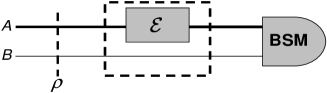
Figure 5: Schematic diagram of the DCQD scheme. The system and the ancilla are prepared in one of the input states as in Table 2, and after subjecting the system to the map $\mathcal{E}$, the combined system is measured in the Bell-state basis.

In order to acquire complete information about the coherence elements of the unknown dynamical map $\mathcal{E}$, we perform an appropriate change of basis by preparing the input states $H^{A}H^{B}|\Phi_{\alpha}^{+}\rangle$ and $S^{A}S^{B}H^{A}H^{B}|\Phi_{\alpha}^{+}\rangle$, which are the eigenvectors of the stabilizer operators $X^{A}X^{B}$ and $Y^{A}Y^{B}$. Here $H$ and $S$ are single-qubit Hadamard and phase gates acting on the systems $A$ and $B.$ At the output, we measure the stabilizers and a corresponding normalizer, e.g., $Z^{A}Z^{B}$, which are again equivalent to a standard BSM, and can be expressed by measuring the Hermitian operators $P_{\Phi^{+}}\pm P_{\Psi^{+}}$ and $P_{\Phi^{-}}\pm P_{\Psi^{-}}$ (for the input state $H^{A}H^{B}|\Phi_{\alpha}^{+}\rangle)$, and $P_{\Phi^{+}}\pm P_{\Psi^{-}}$ and $P_{\Phi^{-}}\pm$ $P_{\Psi^{+}}$ (for the input state $S^{A}S^{B}H^{A}H^{B}|\Phi_{\alpha}^{+}\rangle$). Figure 5 illustrates the DCQD scheme.

Overall, in DCQD we only need a single fixed measurement apparatus capable of performing a Bell state measurement, for a complete characterization of the dynamics. This measurement apparatus is used in four ensemble measurements each corresponding to a different input state. Figure 5 and Table 2 summarize the preparations required for DCQD in the single qubit case. This table implies that the required resources in DCQD are as follows: (a) preparation of a maximally entangled state (for population characterization), (b) preparation of three other (non-maximally) entangled states (for coherence characterization), and (c) a fixed Bell-state analyzer.

Our presentation of the DCQD algorithm assumes ideal (i.e., error-free) quantum state preparation, measurement, and ancilla channels. However, these assumptions can all be relaxed in certain situations, in particular when the imperfections are already known. A discussion of these issues is beyond the scope of this work and will be the subject of a future publication MasoudAli .

Table 2: One possible set of input states and measurements for direct characterization of quantum dynamics ($\bm{\chi}$) for a single qubit. Here $|\Phi^{+}_{\alpha}\rangle=\alpha|00\rangle+\beta|11\rangle$ ($|\alpha|\neq 0,1/\sqrt{2}$), $|\Phi^{+}_{\alpha}\rangle_{X(Y)}=\alpha|++\rangle_{X(Y)}+\beta|--\rangle_{X(Y)}$ ($|\alpha|\neq 0,1/\sqrt{2}$ and $\text{Im}(\alpha\bar{\beta})\neq 0$) and $\{|0\rangle,|1\rangle\}$, $\{|\pm\rangle_{X}\}$, $\{|\pm\rangle_{Y}\}$ are eigenstates of the Pauli operators $Z$, $X$, and $Y$. The fourth column shows the BSM measurement equivalent to stabilizer + normalizer measurements.

input state	Measurement			output $mn$
	Stabilizer	Normalizer	BSM	($\chi_{mn}$)
$|\Phi^{+}\rangle$	$Z^{A}Z^{B},X^{A}X^{B}$	N/A	$P_{\Psi^{\pm}},P_{\Phi^{\pm}}$	00,11,22,33
$|\Phi^{+}_{\alpha}\rangle$	$Z^{A}Z^{B}$	$X^{A}X^{B}$	$P_{\Phi^{+}}\pm P_{\Phi^{-}},P_{\Psi^{+}}\pm P_{\Psi^{-}}$	03,12
$|\Phi^{+}_{\alpha}\rangle_{X}$	$X^{A}X^{B}$	$Z^{A}Z^{B}$	$P_{\Phi^{+}}\pm P_{\Psi^{+}},P_{\Phi^{-}}\pm P_{\Psi^{-}}$	01,23
$|\Phi^{+}_{\alpha}\rangle_{Y}$	$Y^{A}Y^{B}$	$Z^{A}Z^{B}$	$P_{\Phi^{+}}\pm P_{\Psi^{-}},P_{\Phi^{-}}\pm P_{\Psi^{+}}$	02,13

VI Discussion and Resource Comparison

Table 3: Required physical resources for the QPT schemes: Standard Quantum Process Tomography (SQPT), Ancilla-Assisted Process Tomography (AAPT) using joint separable measurements (JSM), using mutual unbiased bases measurements (MUB), using generalized measurements (POVM), and Direct Characterization of Quantum Dynamics (DCQD).

Scheme		$\text{dim}({\mathcal{H}})$	${N}_{\text{inputs}}$	${N}_{\text{meas./input }}$	${N}_{\text{exp.}}$	measurements	required interactions
SQPT		$2^{n}$	$4^{n}$	$4^{n}$	$16^{n}$	1-qubit	single-body
AAPT	JSM	$2^{2n}$	1	$16^{n}$	$16^{n}$	joint 1-qubit	single-body
	MUB	$2^{2n}$	1	$4^{n}+1$	$4^{n}+1$	MUB	many-body
	POVM	$2^{4n}$	1	1	$1$	POVM	many-body
DCQD		$2^{2n}$	$4^{n}$	1	$4^{n}$	BSM	single- and two- body

In this section we present a discussion and comparison of the various QPT schemes described in the previous sections, and highlight the important features of each scheme, as illustrated in Tables 3 and 4. The goal is to provide a (physical) resource analysis and guide for choosing the appropriate QPT scheme, when available resources and the particular system of interest are taken into consideration.

VI.1 Scaling of the Required Number of Experimental Configurations with the Number of Qubits

For characterizing a quantum dynamical map on $n$ qubits we usually perform measurements corresponding to a tensor product of the measurements on the individual qubits. An important example is a quantum information processing unit with $n$ qubits. DCQD requires a total of $4^{n}$ experimental configurations for a complete characterization of the dynamics, where the total number of experimental configurations is defined as the number of input states times the number of non-commuting measurements per input—see Table 3. This is a quadratic advantage over SQPT and separable AAPT, both of which require a total of $16^{n}$ experimental configurations. However for quantum systems without controllable two-qubit operations, implementation of the DCQD scheme is hard, here SQPT is the most efficient scheme.

In principle, the required state tomography in AAPT could also be realized by non-separable (global) quantum measurements. These measurements can be performed either in the same Hilbert space, with $4^{n}+1$ MUB measurements, or in a larger Hilbert space, with a single generalized measurement. Both methods require many-body interactions among $2n$ qubits, which are not naturally available. For the AAPT scheme using MUB measurements, one can simulate the required many-body interactions using a quantum circuit comprising $\mathcal{O}(n^{2})$ $[\mathcal{O}(n^{3})]$ single and two-qubit quantum elementary gates, under the assumption of available non-local [local] two-body interactions. On the other hand, in DCQD the only required operations are Bell-state measurements, each of which requires one cnot and a Hadamard gate. This results in a linear, $\mathcal{O}(n)$, scaling of necessary quantum operations for realization of each experimental configuration in DCQD—see Table 4.

In general, in the $2^{2n}$-dimensional Hilbert space of the $2n$ qubits of the system and the ancilla, one could devise intermediate strategies for AAPT using different combinations of single-, two-, and many-body measurements. The number of experimental configurations in such methods ranges from $4^{n}+1$ to $16^{n}$, which is always larger than that of DCQD, which requires $4^{n}$ BSM setups. Therefore, in the given Hilbert space of $n$ qubits and $n$ ancillas, DCQD requires fewer experimental configurations than all other known QPT schemes. In this sense, DCQD has an advantage over AAPT in a Hilbert space of the same dimension. Moreover, using DCQD one can transfer $\log_{2}2^{2n}$ bits of classical information between two parties, Alice and Bob mohseni-dcqd1 , which is optimal according to the Holevo bound nielsen-book . This is a similar context to the quantum dense coding protocol nielsen-book . Alice can realize the task of sending classical information to Bob by applying one of $2^{2n}$ unitary operator basis elements to the $n$ qubits in her possession and then send them to Bob. Bob can decode the message by a single measurement on his $2n$ qubits using the DCQD scheme. In other words, the total number of possible independent outcomes in each measurement in DCQD is $2^{2n}$, which is exactly equal to the number of independent degrees of freedom for a $2n$-qubit system. Therefore, a maximal amount of information can be extracted in each measurement in DCQD, which cannot be improved upon by any other possible QPT strategy in the same Hilbert space.

For characterizing the dynamics of $n$ qubits in a single generalized (POVM) measurement unambiguously, a Hilbert space of dimension at least $2^{4n}$ is required. In order to implement such a POVM, one needs to realize a global normal operator (a single universal quantum observable) acting on the joint system-ancilla Hilbert space, of the form of Eqs. (11) and (13). Such generic operators cannot be simulated in a polynomial number of steps. It is known nielsen-book that in general at least $\mathcal{O}(4^{2n})$ single- and two-qubit basic operations are needed to simulate such general many-body operations acting on $2n$ qubits.

VI.2 Accuracy Considerations

Due to the finiteness of the number of measurements that can be performed in practice when estimating an ensemble average, it is evident that estimation of an unknown quantum map through any of the QPT schemes gives rise to some error. Such statistical errors can in principle be reduced by increasing the size of ensembles. A relevant question in QPT discussions is then how the accuracy of estimations in different QPT schemes depends on the ensemble size ($N$). Finite size scaling behavior of this accuracy (or error) can provide another practical figure-of-merit for comparison of different QPT schemes. Here, our discussion is just tangential and very incomplete so that it just aims at showing just a rough picture of the issue. A complete investigation of the finite-size errors is not our goal in this paper. Another issue that we partially address here is numerical error due to the inversion required in some QPT schemes.

VI.2.1 Finite Ensemble-Size Effects

There is a huge literature regarding analysis quantum estimation errors or quantum statistics jezekml ; hradil-ml ; hradil-rehacek-prl ; kosut-ml ; buzek-maxent ; sacchi ; buzek-bayesian ; blume ; blume2 ; ziman ; rohde ; helstrom-bk ; holevo-bk ; braunstein-caves-prl ; hayashi2 ; gill-massar ; barndroff-gill ; acin-jane-vidal ; matsumoto-CR ; ballester-pra ; bagan ; ballester-thesis ; metrology ; braunstein-nature ; hayashi1 ; brody-hughston ; Qchernoffbound ; nussb ; deburgh ; qchernoffbound2 . Our aim here is to give a very brief discussion of estimation errors in different QPT schemes through a special example. At the end of this subsection we go a bit further and provide a sketchy discussion of more standard figures-of-merit. However, a more complete investigation of this subject is beyond the goals of this paper and needs a separate study per se.

In all QPT schemes measurements are performed of one or more observables $\{O_{k}^{(X)}\}_{k=1}^{K_{X}}$, where $X$ denotes the scheme: $X\in\{$SQPT, AAPT-JSM, AAPT-MUB, AAPT-POVM, DCQD$\}$. E.g., $K_{\text{AAPT-JSM}}=16^{n}$ (all operator basis for the entire Hilbert space of system and ancilla), $K_{\text{AAPT-POVM}}=1$ (the universal observable $\Omega$), $K_{\text{DCQD}}=4^{n}$ ($4$ Bell state measurements per principal qubit, one for the superoperator population, three for the coherences—here it makes no difference if measurements commute). For notational simplicity let us omit the $(X)$ superscript. Each observable (given scheme $X$) has a spectral decomposition: $O_{k}=\sum_{i=0}^{\nu_{k}-1}\lambda_{i}^{(k)}P_{i}^{(k)}$, where $\lambda_{i}^{(k)}$ are the eigenvalues and $P_{i}^{(k)}$ are projection operators. The number $\nu_{k}$ of distinct projectors is the number of possible measurement outcomes for a given observable $O_{k}$ (which is typically the dimension of the relevant Hilbert space). E.g., in AAPT-POVM (where there is only a single observable), $\nu=16^{n}$, and in DCQD $\nu_{k}=4^{n}$ for all $k$ ($n$-fold tensor product of Bell state measurements on qubit pairs). We can also interpret $\nu_{k}$ as the dimension of the probability space associated with a random variable $Y_{k}$ that can take values $i\in\{0,\ldots,\nu_{k}-1\}$.

Table 4: Resource analysis of the QPT scheme (for the case in which the probabilities $\{p^{(k)}_{i}\}$ are distributed uniformly): Standard Quantum Process Tomography (SQPT), Ancilla-Assisted Process Tomography using joint separable measurements (JSM), using mutual unbiased bases measurements (MUB), using generalized measurements (POVM), and Direct Characterization of Quantum Dynamics (DCQD).

Scheme		${N}_{\text{exp.}}$	1-qubit gates/meas.	2-qubit gates/meas.	$N_{\text{gates/meas.}}$	$N_{\text{overall}}$
SQPT		$16^{n}$	$\mathcal{O}(n)$	N/A	${\mathcal{O}}(n)$	${\mathcal{O}}(n16^{n})$
AAPT	JSM	$16^{n}$	$\mathcal{O}(n)$	$\mathcal{O}(n)$	${\mathcal{O}}(n)$	${\mathcal{O}}(n16^{n})$
	MUB	$4^{n}+1$	$\mathcal{O}(n^{2})$	$\mathcal{O}(n^{2})~{}[\mathcal{O}(n^{3})]$	${\mathcal{O}}(n^{2})~{}[{\mathcal{O}}(n^{3})]$	${\mathcal{O}}(n^{2}4^{n})~{}[{\mathcal{O}}(n^{3}4^{n})]$
	POVM	$1$	${\mathcal{O}}(4^{2n})$	${\mathcal{O}}(4^{2n})$	${\mathcal{O}}(4^{2n})$	${\mathcal{O}}(4^{2n})$
DCQD		$4^{n}$	$\mathcal{O}(n)$	$\mathcal{O}(n)$	${\mathcal{O}}(n)$	${\mathcal{O}}(n4^{n})$

Given an observable $O_{k}$, we must be able to unambiguously determine the index $i$ of which projection operator (or eigenvalue) was measured. For example, when we measure the Pauli operator $Z$, the projectors (eigenvalues) are $P_{0}=|0\rangle\langle 0|$ ($\lambda_{0}=1$) and $P_{1}=|1\rangle\langle 1|$ ($\lambda_{0}=-1$), and we must have a device (e.g., a Stern-Gerlach detector) which unambiguously reveals whether the final state has spin up ($P_{0}$) or down ($P_{1}$). In other words, the raw experimental outcomes are detector clicks in bins that count how many times $n_{i}^{(k)}$ each index $i$ has been obtained. The resulting empirical frequencies $\{f_{i}^{(k)}\equiv n_{i}^{(k)}/N_{k}\}$, where $N_{k}=\sum_{i=0}^{\nu_{k}-1}n_{i}^{(k)}$, are approximations to the true probabilities $\{p_{i}^{(k)}\}$ of detector clicks: $p_{i}^{(k)}=\mathrm{Tr}[\mathcal{E}(\rho)P_{i}^{(k)}]$. In terms of the random variable description mentioned above, we have $\Pr(Y_{k}=i)=p_{i}^{(k)}$.

For a given observable $O_{k}$, repetition of the experiment or increase in the sample size $N_{k}$ can reduce the error in the probability inference $\Delta_{i}^{(k)}\equiv|p_{i}^{(k)}-f_{i}^{(k)}|$. However, we are in general interested in the expectation values of the observables $O_{k}$, that can be obtained from the probability distribution $\{p_{i}^{(k)}\}_{i=0}^{\nu_{k}-1}$. I.e., we would like to know the true mean $\langle O_{k}\rangle\equiv\mathrm{Tr}[\mathcal{E}(\rho)O_{k}]=\sum_{i=0}^{\nu_{k}-1}\lambda_{i}^{(k)}p_{i}^{(k)}$, which we estimate using the empirical frequencies to get the empirical mean $\mu_{k}\equiv\sum_{i=0}^{\nu_{k}-1}\lambda_{i}^{(k)}f_{i}^{(k)}$. The central limit theorem kallenberg (or the Chernoff inequality probability ) states that in the limit $N_{k}\rightarrow\infty$ the probability that the empirical mean $\mu_{k}$ is far from the expected value $\langle O_{k}\rangle$, is very small. More precisely, defining the true standard deviation as usual as $\sigma_{k}\equiv\sqrt{\langle O_{k}^{2}\rangle-\langle O_{k}\rangle^{2}}$ [where $\langle O_{k}^{2}\rangle\equiv\sum_{i=0}^{\nu_{k}-1}(\lambda_{i}^{(k)})^{2}p_{i}^{(k)}$], and letting $z_{\alpha/2}$ be the cutoff for the upper tail of the normal distribution N$(\langle O_{k}\rangle,\sigma_{k}^{2})$ having probability $\alpha/2$, we have asymptotically:$\ \Pr(|\langle O_{k}\rangle-\mu_{k}|\leqslant\frac{z_{\alpha/2}}{\sqrt{N_{k}}})=1-\alpha$. Here $\alpha$ represents the confidence interval. This result allows us to compare the estimates of any two means, by equating their confidence intervals. By replacing the true standard deviation by the empirical one, i.e., by $\xi_{k}\equiv\sqrt{\langle\mu^{2}\rangle_{k}-\mu_{k}^{2}}$ where $\langle\mu^{2}\rangle_{k}\equiv\sum_{i=0}^{\nu_{k}-1}(\lambda_{i}^{(k)})^{2}f_{i}^{(k)}$ (an excellent approximation in large samples), we have

$$\frac{\xi_{k}^{(X)}}{\sqrt{N_{k}^{(X)}}}=\frac{\xi_{k^{\prime}}^{(X^{\prime})}}{\sqrt{N_{k^{\prime}}^{(X^{\prime})}}}$$ (18)

as the criterion for having a confidence interval of equal length around the two sample means $\mu_{k}^{(X)}$ and $\mu_{k}^{(X^{\prime})}$, i.e., to contain the unknown true means $\langle O_{k}\rangle$ and $\langle O_{k^{\prime}}\rangle$ with equal probability. Here we have reintroduced the QPT label (superscript $X$) to stress that this criterion holds for the comparison of estimates of any two means, across both $k$ and $X$. This result shows that, assuming the standard deviations do not scale with $\nu_{k}$, equal confidence in estimates of two expectation values of two observables $O_{k}^{(X)}$ and $O_{k^{\prime}}^{(X^{\prime})}$ simply requires equal sample sizes $N_{k}^{(X)}$ and $N_{k^{\prime}}^{(X^{\prime})}$.

However, let us note that the above statistical argument is rigorous only in the limit $N_{k}\rightarrow\infty$. That the situation is different for finite sample sizes can be appreciated via the following examples, for which we first recall the Chernoff inequality probability . The version of this inequality which is best suited to our present purpose is as follows. Assume that an event $\gamma$ occurs with the true probability $p(\gamma)$. We estimate this probability by performing $N$ independent trials. The inferred probability is then $p_{N}(\gamma)=n_{N}(\gamma)/N$, where $n_{N}(\gamma)$ is the number of occurrences of $\gamma$ in the trials. Then for any $\Delta\in[0,1]$ the Chernoff inequality is

$$\text{Pr}\left(|p_{N}(\gamma)-p(\gamma)|\geqslant\Delta p(\gamma)\right)\leqslant e^{-p(\gamma)N\Delta^{2}/3}.$$ (19)

An immediate result of this inequality is the following. Let

$$N(\gamma;\Delta,\epsilon)\equiv\frac{3}{p(\gamma)\Delta^{2}}\log\frac{1}{\epsilon}.$$ (20)

Then for any $\Delta,\epsilon\in[0,1]$, if $N\geqslant N(\gamma;\Delta,\epsilon)$, then with probability greater than $1-\epsilon$ we have $|p_{N}(\gamma)-p(\gamma)|/p(\gamma)\leqslant\Delta$. Roughly, if we wish $p_{N}(\gamma)$ to be within an error of at most $\Delta$ from $p(\gamma)$, this can happen with a probability greater than $1-\epsilon$ (for some $\epsilon$) when we perform at least $N(\gamma;\Delta,\epsilon)$ trials. It follows that a highly accurate estimation ($\Delta,\epsilon\rightarrow 0$) requires many ($N\rightarrow\infty$) trials. In standard statistical error analysis $\Delta$ is usually taken to be the standard deviation $\sigma_{N}$ or at most $2\sigma_{N}$.

From Eq. (20) it is evident that if the probabilities $\{p_{i}\}$ does not depend on the dimension of the Hilbert space ($n$) the number of repetitions to fulfill an error $\epsilon$ would not either—this number will only have a logarithmic dependence on the error $\epsilon$. This implies that there are cases in which the statistics can be built up with a constant overhead in ensemble size–up to the logarithmic dependence on the error. This can have highly useful and efficient applications for QPT in such cases. Nonetheless, it would be important to point out an intricate pitfall in (incautious) too general conclusions. To this aim, here we want to analyze a somewhat pathological example in which efficiency cannot be concluded from Eq. (20). Let us assume that we are dealing with fairly uniform probability distributions $\{p_{i}^{(k)}\}_{i=0}^{\nu_{k}-1}$ and compare two situations: tossing a coin (two possible outcomes: $\nu_{1}=2$) and estimating the probability distribution of a random variable with $\nu_{2}=10^{10}$ different possible outcomes. In the case of the coin it is clear that after $N=10^{8}$ tosses we will have a pretty good idea about the probabilities $p_{H}^{(1)}$ and $p_{T}^{(1)}$ of heads vs tails. On the other hand, for the other random variable, after $N=10^{8}$ measurements we will have not yet sampled the entire space of possible outcomes, so will not have been able to gather statistics representative of all probabilities $p_{i}^{(2)}$ (some outcomes will not have ever occurred, thus their probabilities cannot be estimated). Consequently, we will not be able to accurately estimate any means. However, from Eq. (20), with the uniform probability distribution assumption $p_{i}^{(k)}=1/\nu_{k}$, we obtain

$$N_{k}\geqslant N(\Delta,\epsilon)=3\frac{\nu_{k}}{\Delta^{2}}\log\frac{1}{\epsilon}\equiv\nu_{k}C(\Delta,\epsilon),$$ (21)

In other words, for accurate estimation of means in the case of fairly uniform probability distributions it is sufficient to have $N_{k}\geqslant C(\Delta,\epsilon)\nu_{k}$, where the prefactor $C(\Delta,\epsilon)$ encompasses both the estimation error $\Delta$ and the probability $1-\epsilon$ to achieve that error. We call condition (21) the “good statistics” condition. It is important to note that this conclusion depends strongly on the assumption of fairly uniform probability distributions. Indeed, consider the case where the random variable with $10^{10}$ different possible outcomes is very strongly peaked at two values $\{i_{1},i_{2}\}$. In this case it behaves effectively like a coin, and we do not need $N\geqslant 10^{10}$.

We thus see that a comparison of the different QPT methods on the basis of fixed mean-estimation error will depend strongly on the properties of the underlying probability distributions $\{\{p_{i}^{(k)}\}_{i=0}^{\nu_{k}-1}\}_{k=1}^{K_{X}}$. A thorough study of the properties of these probability distributions as a function of QPT method $X$ is beyond the scope of this paper. However, let us speculate on what would happen if the assumption of fairly uniform distributions were to hold for all $k$ and $X$. The total number of ensemble measurements becomes

$$N^{(X)}=\sum_{k=1}^{K_{X}}N_{k}^{(X)}\cdot N_{\text{inputs},k}^{(X)},$$ (22)

where $N_{\text{inputs},k}^{(X)}$ is the number of initial states needed per observable $k$ for a given QPT scheme $(X)$, and $N_{k}^{(X)}$ is found from the good statistics condition (21), with $\nu_{k}$ replaced by $\nu_{k}^{(X)}$. We can read off the values of $N_{\text{inputs},k}^{(X)}$ and $K_{X}$ from the second and third columns of Table 3, respectively. The values of $\nu_{k}^{(X)}$ are as follows. In the case of $X$=SQPT and AAPT-JSM the observables are all one-dimensional projectors so that $\nu_{k}=1$ $\forall k$. In the case of $X$=AAPT-MUB there are $2n$ qubits (i.e., a $4^{n}$-dimensional Hilbert space) and one performs quantum state tomography at the output by measuring a set of noncommuting $4^{n}+1$ observables of the MUB basis, where each member of the MUB basis has a spectral resolution over $\nu_{k}=4^{n}-1$ independent projective measurements. We already noted above that $\nu_{k}^{(X)}=4^{n}$ and $16^{n}$ for $X$=DCQD, and AAPT-POVM, respectively. We observe that, for fairly uniform distributions, $N_{k}^{(X)}$ grows exponentially with respect to the number of qubits $n$ for non-separable process tomography schemes, with AAPT-MUB and AAPT-POVM at a distant disadvantage due to the inherent depth of their quantum circuits for simulating many-body interactions in each measurement (see the fourth column of Table 4). Collecting the results above, however, it follows from Eq. (22) that the total number of ensemble measurements $N^{(X)}$ scales as $16^{n}$ in all QPT methods, to within a factor $C^{(X)}(\Delta,\epsilon)$.

How would the number of ensemble measurements, $N_{k}^{(X)}$, change if the distributions are sharply peaked? For separable schemes, e.g., SQPT and AAPT-JSM, this would not result in any difference, since we already have $\nu_{k}^{(X)}=1$. However, for non-separable schemes this would lead to substantial reduction of measurements since we would be dealing with effectively fixed-dimensional probability distribution spaces, e.g., $\nu_{k}^{(X)}=\text{const.}$, instead of an exponential function of the number of qubits. Hence the question of the properties of the probability distributions $\{\{p_{i}^{(k)}\}_{i=0}^{\nu_{k}-1}\}_{k=1}^{K_{X}}$ is indeed important and will be the subject of a future study.

VI.2.2 Discussion of Figure-of-Merit

One of the standard approaches in quantum estimation and quantum statistics to address estimation errors is via the Cramér-Rao bound (CRB) braunstein-caves-prl ; gill-massar ; ballester-thesis ; kosut-ml . Following Ref. kosut-ml , the CRB can be described as follows. Let us assume that $\{\chi^{(\text{R})}_{mn}\}\in\mathbb{R}^{N^{4}}$ are the true (real-valued independent) parameters of $\bm{\chi}$ that are supposed to be estimated from a measurement data set $\mathcal{D}_{X}$ obtained through the scheme $X$ - we remove the superscript R in the sequel without any risk of confusion. The true negative logarithmic likelihood function of the system generating that true data is defined by

$$\log\mathcal{L}^{(X)}=-\sum_{k=1}^{K_{X}}\sum_{i=0}^{\nu_{k}-1}n^{(k)}_{i}\log p^{(k)}_{i},$$

where $n^{(k)}_{i}$ is the number of times the outcome $i$ is obtained from $\ell_{k}$ measurements of $O_{k}$ (total of $\sum_{k}\ell_{k}$ measurements) and $\langle n^{(k)}_{i}\rangle=p^{(k)}_{i}\ell_{k}$ (where $\langle~{}\rangle$ is the quantum average). If $\widehat{\bm{\chi}}\in\mathbb{R}^{N^{4}}$ is an unbiased estimate of $\bm{\chi}$, i.e., $\langle\widehat{\bm{\chi}}\rangle=\bm{\chi}$, the covariance of the estimate $\text{cov}(\widehat{\bm{\chi}})=\langle(\hat{\bm{\chi}}-\bm{\chi})(\widehat{\bm{\chi}}-\bm{\chi})^{T}\rangle$ satisfies the following matrix inequality:

$$\left(\begin{array}[]{cc}\text{cov}(\widehat{\bm{\chi}})&I\\ I&\mathcal{F}(\bm{\chi})\end{array}\right)\geqslant 0,$$ (25)

where $\mathcal{F}$ is the Fisher information matrix defined as

$$\mathcal{F}_{mn,m^{\prime}n^{\prime}}(\bm{\chi}) = \langle\nabla_{\bm{\chi}^{\prime}\bm{\chi}^{\prime}}\log\mathcal{L}^{(X)}|_{\bm{\chi}}\rangle$$

$$= \langle\frac{\partial\log p^{(k)}_{i}}{\partial\chi_{mn}}\frac{\partial\log p^{(k)}_{i}}{\partial\chi_{m^{\prime}n^{\prime}}}|_{\bm{\chi}}\rangle.$$

Provided that $\mathcal{F}(\bm{\chi})$ is positive and invertible, Eq. (25) gives the following well-known form of the CRB:

$$\text{cov}(\widehat{\bm{\chi}})\geqslant\mathcal{F}^{-1}(\bm{\chi}).$$ (26)

Taking the trace of both sides and noting that $\text{var}(\widehat{\bm{\chi}})=\text{Tr}[\text{cov}(\widehat{\bm{\chi}})]$, one can also find a scalar form for this equation. Equation (26) means that for any unbiased estimator the error is lower-bounded by the inverse of the Fisher information. The Fisher information matrix is indeed a measure of information about $\bm{\chi}$ that exists in the data $\mathcal{D}_{X}$. The special feature and indeed the power of this bound is that it is independent of how the estimate is obtained, for $\mathcal{F}$ is independent of the estimation mechanism. For the case of single-parameter estimation, the CRB can always be achieved asymptotically by using maximum likelihood (ML) estimation hradil-rehacek-prl ; ballester-thesis ; kallenberg . That is, as the amount of data increases the ML estimate approaches the true answer with the error bars equal to those given by the CRB. However, for multi-parameter estimation there is, in general, no optimal estimator that can achieve this bound. See Ref. ballester-thesis and references therein for more information about the CRB, its quantum version, and its application to quantum state estimation. The above discussion may suggest that the (inverse of the) Fisher information matrix can be taken as a good figure-of-merit for a quantum estimation process. However, the very nature of independence from estimation method means that the Fisher information matrix is not so useful for the purpose of comparing different QPT schemes—our goal in this paper.

A more promising and physically-motivated approach, that justifies using the Chernoff bound for the purpose of quantum state/process estimation as we did earlier, has been proposed very recently, and is called the quantum Chernoff bound (QCB) Qchernoffbound ; nussb ; deburgh ; qchernoffbound2 . The physical interpretation of this quantity is as follows: assuming that we have access to all types of measurements—whether local or collective—on all ensembles, the QCB measures the error in distinguishing a state $\rho$ from another state $\widehat{\rho}$. The probability of a wrong inference, i.e., mistaking $\widehat{\rho}$ for $\rho$, has the asymptotic form $P_{e}\sim e^{N\ln\Lambda_{\text{CB}}(\rho,\widehat{\rho})}$, where

$$\Lambda_{\text{CB}}(\rho,\widehat{\rho})=\min_{0\leqslant\alpha\leqslant 1}\text{Tr}[\rho^{\alpha}\widehat{\rho}^{1-\alpha}],$$ (27)

is the QCB, and $0\leqslant\Lambda_{\text{CB}}\leqslant 1$. The maximum is attained for $\rho=\widehat{\rho}$ Qchernoffbound ; deburgh ; qchernoffbound2 . Recently, the QCB has been considered as a natural figure-of-merit in evaluating the performance of different measurement scenarios for qubit tomography deburgh . It also has been used for quantum hypothesis testing and distinguishability between density matrices nussb ; qchernoffbound2 . Considering the fact that a generic $\bm{\chi}$ matrix is formally in the category of density matrices, the application of the QCB can in principle be extended to QPT. That is, one can in principle calculate $\Lambda_{\text{CB}}^{(X)}(\bm{\chi},\widehat{\bm{\chi}})$ for estimation of a quantum process $\bm{\chi}$ through any QPT scheme $X$ and then take an average over all possible processes with a suitable probability measure $\text{d}\mu(\bm{\chi})$ deburgh ; qchernoffbound2 . The average QCB

$$\Lambda^{(X)}_{\text{CB}}=\int\text{d}\mu(\bm{\chi})\sum_{\widehat{\bm{\chi}}}p(\widehat{\bm{\chi}}|\bm{\chi})\Lambda_{\text{CB}}^{(X)}(\bm{\chi},\widehat{\bm{\chi}}),$$ (28)

where $p(\widehat{\bm{\chi}}|\bm{\chi})$ is the probability of estimating $\widehat{\bm{\chi}}$ given the true process $\bm{\chi}$, may prove a more useful figure-of-merit. A more complete analysis, along with possible numerics, that explicitly shows the performance of different QPT schemes (similar to the analysis of Ref. deburgh ), is yet to be performed. One important point, however, is the issue that may be caused by the assumption of availability of all types of measurements (including collective measurements) in this bound and whether they are important in achieving the bound or not. This may in turn complicate usage of this tool as a completely suitable figure-of-merit for a comparative study of different QPT schemes. For completeness, let us mention that a different investigation of physically good figures-of-merit (or distance measures) for quantum operations has also been performed in Ref. gilchrist .

Other characteristics of the QPT schemes may also play significant roles in the propagation of errors in the inferred quantum map $\mathcal{E}$. Indeed, the effect of preparation, i.e., how different input states can affect efficiency of the estimation of unknown maps, must be explored as well - for a recent study see Ref. sudarshan . For the case of AAPT, as explained earlier, it is already known that using maximally entangled input states is favored, because they result in smaller experimental errors than separable states. For DCQD an analysis of how different input states affect performance of the estimation is underway mohseni-rezakhani-aspuru08 . Without a full understanding of the role of preparation, the scaleup of physical resources in different QPT strategies for finite ensemble sizes remains elusive. This again underlines that a promising direction is to attempt to find a more suitable information-theoretic figure-of-merit that can be used in a comparative finite ensemble-size analysis of the different QPT schemes.

VI.2.3 The Role of Inversion

It should be noted that in order to reconstruct the unknown map $\mathcal{E}$ in a QPT scheme one generally needs to perform an inversion operation which here can be understood as Eq. (12). In particular, in the SQPT and AAPT schemes an inversion on experimental data is inevitable. This inversion may induce an ill-conditioning feature jezekml ; boulant-lindblad , i.e., small errors in experimental outcomes may give rise to large errors in the estimation of $\mathcal{E}$, and can sometimes result in non-positive maps. It should be stressed that quantum dynamics obtained via the usual prescription of unitary evolution followed by a partial trace over the bath, is always positive when the initial state is a valid density matrix. When a positive map is applied outside of its positivity domain it will result in non-positive density matrix. Complete positivity results when in addition one assumes a factorized initial system-bath state. Non-complete positivity is thus a legitimate feature of correlated initial conditions, and non-positivity is a legitimate feature of applying a positive map to states outside of its positivity domain Jordan ; Carteret ; Shabani-Lidar . The problem with ill-conditioning due to inversion is a of a different nature: it is a numerical error that leads to a non-positive or non-completely-positive map. This problem, to a large extent, can be addressed by supplementary data analysis methods, such as ML estimation jezekml ; hradil-ml ; hradil-rehacek-prl ; boulant-lindblad ; kosut-ml ; buzek-maxent ; sacchi , Bayesian state estimation buzek-bayesian ; blume ; blume2 , and other reliable regularization or reconstruction methods ziman ; rohde ; d'ariano-07 . In principle, all known QPT schemes (including DCQD) can be optimized by utilizing such statistical error reduction techniques. Here we will not delve into the details of such methods, as they are applicable on a similar footing to all QPT schemes, and moreover, this issue is beyond the scope of the present paper. However, we would like to emphasize that DCQD is inherently more immune against such inversion-amplified errors. The diagonal elements of a map, as discussed above, are related in DCQD directly to measurement results. For off-diagonal elements a large extent of directness also exists. This can easily be seen, for example, through the determination of $\chi_{03}$ — see Eq.  (16) — in which only the quantities $\chi_{00}$ and $\chi_{33}$ (already obtained from a different experimental configuration) need to be used. That is, the formal inversion necessary in DCQD requires only a small amount of data processing. This, in turn implies that inversion-induced errors are amplified less than in methods requiring a full inversion.

VI.3 Partial Characterization of Quantum Dynamics

An important and promising advantage of DCQD is for use in partial characterization of quantum dynamics, where one cannot afford or does not need to carry out a full characterization of the quantum system under study, or when one has some a priori knowledge about the dynamics. Using indirect QPT methods in such situations is generally inefficient, because one must apply the whole machinery of the scheme (including its inversion) to obtain the desired partial information about the system. On the other hand, the DCQD scheme is inherently applicable to the task of partial characterization of quantum dynamics. In general, one can substantially reduce the total number of measurements when estimating the coherence elements of the superoperator for only specific subsets of the operator basis and/or subsystems of interest. For example, a single ensemble measurement is needed if one wishes to identify only the coherence elements $\chi_{03}$ and $\chi_{12}$ of a particular qubit. In Refs. mohseni-dcqd1 ; mohseni-dcqd2 ; mohseni-rezakhani-aspuru ; mohseni-rezakhani-aspuru08 several examples of partial characterization have been demonstrated. For example it was demonstrated that DCQD enables the simultaneous determination of coarse-grained (semiclassical) physical quantities, such as the longitudinal relaxation time $T_{1}$ and the transversal relaxation (or dephasing) time $T_{2}$. Alternative methods for efficient selective estimation of quantum dynamical maps has been recently developed by utilizing random sampling Emerson07 . The central idea of these methods is symmetrization of a quantum channel by randomization, and then efficient estimation of gate fidelities. The application of such partial/selective process estimation schemes for efficient Hamiltonian identification of open quantum systems is important per se—besides its practical implications—and will be presented elsewhere mohseni-rezakhani-aspuru08 .

VII Concluding Remarks

In the absence of a good, reliable figure-of-merit for the performance of QPT schemes, one cannot provide a fully fair and decisive comparative analysis. In addition, one should also consider the complexity of physical resources associated with noisy/imperfect quantum state preparation and measurements. Nevertheless, in this work we have presented a detailed resource-based comparison of ideal quantum process tomography schemes with respect to overall number of experimental configurations and elementary quantum operations. In general, SQPT is always the best approach for complete estimation of quantum dynamical systems when controlled two-body interactions are not either available or desirable. However, for quantum systems with controllable single- and two-body interactions, we have shown that the DCQD approach is more efficient than SQPT, and all versions of AAPT, in terms of the total number of elementary quantum operations required. For such systems, DCQD appears attractive for near-term applications involving complete verification of small quantum information processing units, especially in trapped-ion and liquid-state NMR systems. For example, the number of required experimental configurations for systems of $3$ or $4$ physical qubits is reduced from $\sim 5\times 10^{3}$ and $\sim 6.5\times 10^{4}$ in SQPT to $64$ and $256$ in DCQD, respectively. Such complete characterization of quantum dynamics is essential for verification of quantum key distribution procedures, teleportation units (in both quantum communication and distributed quantum computation), quantum repeaters, quantum error-correction procedures, and more generally, in any situation in quantum physics where a few particles interact amongst themselves and with a common environment.

- (1) M. A. Nielsen and I. L. Chuang, Quantum Computation and Quantum Information (Cambridge University Press, Cambridge, UK, 2000).
- (2) G. M. D’Ariano, M. G. A. Paris, and M. F. Sacchi, Advances in Imaging and Electron Physics Vol. 128, 205 (2003).
- (3) G. M. D.Ariano and P. Lo Presti, in Quantum State Estimation, edited by M. Paris and J. Reh cek, Lecture Notes in Physics Vol. 649 (Springer-Verlag, Berlin, 2004), p. 297.
- (4) L. M. Artiles, R. D. Gill, and M. I. Guţă, J. R. Statist. Soc. B 67, 109 (2005).
- (5) I. L. Chuang and M. A. Nielsen, J. Mod. Opt. 44, 2455 (1997).
- (6) J. J. Poyatos, J. I. Cirac, and P. Zoller, Phys. Rev. Lett. 78, 390 (1997).
- (7) D. W. Leung, PhD thesis (Stanford University, 2000); J. Math. Phys. 44, 528 (2003).
- (8) G. M. D’Ariano and P. Lo Presti, Phys. Rev. Let. 86, 4195 (2001).
- (9) J. B. Altepeter, D. Branning, E. Jeffrey, T. C. Wei, P. G. Kwiat, R. T. Thew, J. L. O’Brien, M. A. Nielsen, and A. G. White, Phys. Rev. Lett. 90, 193601 (2003).
- (10) G. M. D’Ariano and P. Lo Presti, Phys. Rev. Lett. 91, 047902 (2003).
- (11) A. K. Ekert, C. M. Alves, D. K. L. Oi, M. Horodecki, P. Horodecki, and L. C. Kwek, Phys. Rev. Lett. 88, 217901 (2002).
- (12) P. Horodecki and A. Ekert, Phys. Rev. Lett. 89, 127902 (2002).
- (13) F. A. Bovino, G. Castagnoli, A. Ekert, P. Horodecki, C. M. Alves, and A. V. Sergienko, Phys. Rev. Lett. 95, 240407 (2005).
- (14) J. Emerson, Y. S. Weinstein, M. Saraceno, S. Lloyd, and D. G. Cory, Science 302, 2098 (2003); J. Emerson, R. Alicki, and K. Życzkowski, J. Opt. B: Quantum Semiclass. Opt. 7 S347 (2005).
- (15) H. F. Hofmann, Phys. Rev. Lett. 94, 160504 (2005).
- (16) C. H. Bennett, A. W. Harrow, and S. Lloyd, Phys. Rev. A 73, 032336 (2006).
- (17) M. Mohseni and D. A. Lidar, Phys. Rev. Lett. 97, 170501 (2006).
- (18) M. Mohseni and D. A. Lidar, Phys. Rev. A 75, 062331 (2007).
- (19) M. Mohseni, PhD thesis (University of Toronto, 2006).
- (20) Z. -W. Wang, Y. -S. Zhang, Y. -F. Huang, X. -F. Ren, and G. -C. Guo, Phys. Rev. A 75, 044304 (2007).
- (21) M. Mohseni, A. T. Rezakhani, and A. Aspuru-Guzik, eprint arXiv:0708.0436.
- (22) J. Emerson, M. Silva, O. Moussa, C. Ryan, M. Laforest, J. Baugh, D. G. Cory, and R. Laflamme, Science 317, 1893 (2007); M. Silva, E. Magesan, D. W. Kribs, and J. Emerson, eprint arXiv:0710.1900; A. Bendersky, F. Pastawski, and J. P. Paz, eprint arXiv:0801.0758.
- (23) M. Mohseni, A. T. Rezakhani, and A. Aspuru-Guzik, in preparation.
- (24) A. M. Childs, I. L. Chuang, and D. W. Leung, Phys. Rev. A 64, 012314 (2001).
- (25) N. Boulant, T. F. Havel, M. A. Pravia, and D. G. Cory, Phys. Rev. A 67, 042322 (2003).
- (26) Y. S. Weinstein, T. F. Havel, J. Emerson, and N. Boulant, M. Saraceno, S. Lloyd, and D. G. Cory, J. Chem. Phys. 121, 6117 (2004).
- (27) M. W. Mitchell, C. W. Ellenor, S. Schneider, and A. M. Steinberg, Phys. Rev. Lett. 91, 120402 (2003).
- (28) J. L. O’Brien, G. J. Pryde, A. Gilchrist, D. F. V. James, N. K. Langford, T. C. Ralph, and A. G. White, Phys. Rev. Lett. 93, 080502 (2004).
- (29) S. H. Myrskog, J. K. Fox, M. W. Mitchell, and A. M. Steinberg, Phys. Rev. A 72, 013615 (2005).
- (30) M. Howard, J. Twamley, C. Wittmann, T. Gaebel, F. Jelezko, and J. Wrachtrup, New J. Phys. 8, 33 (2006).
- (31) A. Jamiolkowski, Rep. Math. Phys. 3, 275 (1972); M. D. Choi, Linear Algebr. Appl. 10, 285 (1975).
- (32) P. Arrighi and C. Patricot, Ann. Phys. 311, 26 (2004).
- (33) A. Gilchrist, N. K. Langford, and M. A. Nielsen, Phys. Rev. A 71, 062310 (2005).
- (34) M. A. Nielsen, C. M. Dawson, J. L. Dodd, A. Gilchrist, D. Mortimer, T. J. Osborne, M. J. Bremner, A. W. Harrow, and A. Hines, Phys. Rev. A 67, 052301 (2003).
- (35) S. L. Braunstein, C. M. Caves, R. Jozsa, N. Linden, S. Popescu, and R. Schack, Phys. Rev. Lett. 83, 1054 (1999).
- (36) I. Ivanovič, J. Phys. A 14, 3241 (1981).
- (37) W. K. Wootters and B. D. Fields, Ann. Phys. 191, 363 (1989).
- (38) S. Bandyopadhyay, P. O. Boykin, V. Roychowdhury, and F. Vatan, Algorithmica 34, 512 (2002).
- (39) J. Lawrence, Č. Brukner, and A. Zeilinger, Phys. Rev. A 65, 032320 (2002).
- (40) J. L. Romero, G. Björk, A. B. Klimov, and L. L. Sánchez-Soto, Phys. Rev. A 72, 062310 (2005).
- (41) M. Ziman, eprint quant-ph/0603151.
- (42) M. Mohseni and D. A. Lidar, eprint quant-ph/0604114.
- (43) M. Möttönen and J. J. Vartiainen, in Trends in Quantum Computing Research, edited by S. Shannon (Nova Science Publishers Inc., New York, 2006), p. 149.
- (44) G. M. D’Ariano, Phys. Lett. A 300, 1 (2002).
- (45) G. M. D’Ariano, P. Perinotti, and M. F. Sacchi, Europhys. Lett. 65, 165 (2004).
- (46) C. M. Caves, C. A. Fuchs, and R. Schack, J. Math. Phys. 43, 4537 (2002).
- (47) A. E. Allahverdyan, R. Balian, and Th. M. Nieuwenhuizen, Phys. Rev. Lett. 92, 120402 (2004).
- (48) V. V. Shende, I. L. Markov, and S. S. Bullock, Phys. Rev. A 69, 062321 (2004); E. Knill, eprint quant-ph/9508006.
- (49) R. Jozsa, M. Koashi, N. Linden, S. Popescu, S. Presnell, D. Shepherd, A. Winter, Quant. Inf. Comp. 3, 405 (2003).
- (50) D. Gottesman, PhD thesis (California Institute of Technology, 1997), eprint quant-ph/9705052.
- (51) M. Mohseni and A. T. Rezakhani, in preparation.
- (52) M. Ježek, J. Fiurášek, and Z. Hradil, Phys. Rev. A 68, 012305 (2003).
- (53) Z. Hradil, Phys. Rev. A 55, R1561 (1997).
- (54) Z. Hradil, D. Mogilevtsev, and J. Řeháček, Phys. Rev. Lett. 96, 230401 (2006).
- (55) R. L. Kosut, I. Walmsley, and H. Rabitz, eprint quant-ph/0411093.
- (56) V. Bužek, in Quantum State Estimation, edited by M. Paris and J. Řeháček, Lecture Notes in Physics Vol. 649 (Springer-Verlag, Berlin, 2004), p. 189.
- (57) M. E. Sacchi, Phys. Rev. A 63, 054104 (2001).
- (58) V. Bužek, R. Derka, G. Adam, and P. L. Knight, Ann. Phys. 266, 454 (1998).
- (59) R. Blume-Kohout and P. Hayden, eprint quant-ph/0603116.
- (60) R. Blume-Kohout, eprint quant-ph/0611080.
- (61) M. Ziman, M. Plesch, and V. Bužek, Eur. Phys. J. D 32, 215 (2005).
- (62) P. P. Rohde, G. J. Pryde, J. L. O’Brien, and T. C. Ralph, Phys. Rev. A 72, 032306 (2005).
- (63) G. M. D’Ariano and P. Perinotti, Phys. Rev. Lett. 98, 020403 (2007).
- (64) C. W. Helstrom, Quantum Detection and Estimation Theory (Academic Press, New York, 1976).
- (65) A. S. Holevo, Probabilistic and Statistical Aspects of Quantum Theory (North-Holland, Amsterdam, 1982).
- (66) S. L. Braunstein and C. M. Caves, Phys. Rev. Lett. 72, 3439 (1994); S. L. Braunstein, C. M. Caves, and G. J. Milburn, Ann. Phys. 247, 135 (1996).
- (67) M. Hayashi, J. Phys. A: Math. Gen. 31, 4633 (1998).
- (68) R. D. Gill and S. Massar, Phys. Rev. A 61, 042312 (2000).
- (69) O. E. Barndroff-Nielsen and R. D. Gill, J. Math. A: Math. Gen. 33 4481 (2000).
- (70) A. Acín, E. Jané, and G. Vidal, Phys. Rev. A 64, 050302 (2001).
- (71) K. Matsumoto, J. Phys. A: Math. Gen. 35, 3111 (2002).
- (72) M. A. Ballester, Phys. Rev. A 69, 022303 (2004).
- (73) E. Bagan, A. Monras, and R. Muñoz-Tapia, Phys. Rev. A 71, 062318 (2005).
- (74) M. A. Ballester, PhD thesis (Utrecht University, 2005).
- (75) V. Giovannetti, S. Lloyd, and L. Maccone, Phys. Rev. Lett. 96, 010401 (2006).
- (76) S. L. Braunstein, Nature 440, 617 (2006).
- (77) M. Hayashi, in Quantum Computation and Information: From Theory to Experiment, edited by H. Imai and M. Hayashi, Topics in Applied Physics Vol. 102 (Springer-Verlag, Berlin, 2006), p. 45.
- (78) D. C. Brody and L. P. Hughston, Phys. Rev. Lett. 77, 2851 (1996).
- (79) K. M. R. Audenaert, J. Calsamiglia, R. Muñoz-Tapia, E. Bagan, Ll. Masanes, A. Acin, and F. Verstraete, Phys. Rev. Lett. 98, 160501 (2007).
- (80) M. Nussbaum and A. Szkola, eprint quant-ph/0607216.
- (81) M. de Burgh, N. K. Langford, A. C. Doherty, and A. Gilchrist, Phys. Rev. A 77, 032311 (2008).
- (82) J. Calsamiglia, R. Muñoz-Tapia, Ll. Masanes, A. Acin, and E. Bagan, eprint arXiv:0708.2343.
- (83) O. Kallenberg, Foundations of Modern Probability (Springer-Verlag, New York, 1997).
- (84) R. Tempo, G. Calafiore, and F. Dabbene, Randomized Algorithms for Analysis and Control of Uncertain Systems (Springer, Berlin, Heidelberg, 2005).
- (85) A. -M. Kuah, K. Modi, C. A. Rodríguez-Rosario, and E. C. G. Sudarshan, Phys. Rev. A 76, 042113 (2007).
- (86) T. F. Jordan, A. Shaji, and E. C. G. Sudarshan, Phys. Rev. A 70, 052110 (2004).
- (87) H. Carteret, D. R. Terno, and K. Życzkowski, eprint quant-ph/0512167.
- (88) A. Shabani and D. A. Lidar, eprint quant-ph/0610028 and arXiv:0708.1953.