An Information-Theoretic Approach to Quantum Theory, I:
The Abstract Quantum Formalism

Abstract

In this paper and a companion paper, we attempt to systematically investigate the possibility that the concept of information may enable a derivation of the quantum formalism from a set of physically comprehensible postulates. To do so, we formulate an abstract experimental set-up and a set of assumptions based on generalizations of experimental facts that can be reasonably taken to be representative of quantum phenomena, and on theoretical ideas and principles, and show that it is possible to deduce the quantum formalism. In particular, we show that it is possible to derive the abstract quantum formalism for finite-dimensional quantum systems and the formal relations, such as the canonical commutation relationships and Dirac’s Poisson Bracket rule, that are needed to apply the abstract formalism to particular systems of interest. The concept of information, via an information-theoretic invariance principle, plays a key role in the derivation, and gives rise to some of the central structural features of the quantum formalism.

I Introduction

Over the last two decades, a number of authors have expressed the view that our efforts to develop an understanding of quantum theory are impeded by a lack of understanding of the physical origin of the quantum formalism, and that our efforts would thereby be significantly aided by a systematic derivation of the formalism from a set of physically comprehensible assumptions Rovelli96 ; Popescu-Rohrlich97 ; Fuchs02 . Furthermore, several authors have proposed that the concept of information may be the key, hitherto missing, ingredient which, if appropriately applied and formalized, might make such a derivation possible Wheeler89 ; Rovelli96 ; Summhammer99 ; Zeilinger99 ; Fuchs02 .

The proposal that information might enable a derivation of quantum formalism rests, to a significant degree, upon the recognition that the concept of information plays a new and fundamental role in quantum physics. One way to see this is as follows. In classical physics, an experimenter presented with a system in an unknown state can, in principle, perform an ideal measurement upon the system which gives perfect knowledge about the state of the system. Hence, there is no fundamental distinction between the state and an ideal experimenter’s knowledge of the state. In quantum physics, however, an ideal measurement (or even a finite number of such measurements performed upon an ensemble of identically-prepared systems) provides only partial knowledge about the unknown state of a quantum system. Hence, in sharp contrast to the situation in classical physics, a fundamental distinction is drawn between the state and the knowledge that the experimenter can conceivably have of it. The concept of information then immediately assumes a fundamental role through the natural attempt to quantitatively relate the two: ‘How much information has been obtained by the experimenter about the state?’

One of the earliest attempts to explore the role of information is due to Wootters Wootters80 . Suppose that Alice has a Stern-Gerlach apparatus oriented at angle $(\theta,\phi)$, and attempts to communicate the angle $\theta$ to Bob using spin-$1/2$ particles as follows. Alice prepares $n$ spin-$1/2$ particles in the state $|+\rangle_{\theta,\phi}$ using her Stern-Gerlach apparatus, and sends the particles to Bob, who measures them using a vertically-aligned Stern-Gerlach apparatus. The data he obtains provides information about the outcome probabilities, $P_{1},P_{2}$, of the measurement, where $P_{1}$ is the probability of a spin emerging in the positive channel. Since, from quantum theory, $P_{1}=\cos^{2}(\theta/2)$, Bob thereby gains information about $\theta$. However, we can now ask the question: suppose we did not know quantum theory, and instead simply regard the experimental arrangement as a way for Bob to learn about $\theta$ by observing the frequencies of the two possible outcomes of his Stern-Gerlach apparatus; what function $P_{1}(\theta)$ would maximize the amount of information obtained by Bob about $\theta$ for given $n$? Wootters finds that, if the information is quantified using the Shannon information measure, then, in the limit as $n\rightarrow\infty$, the function is $P_{1}(\theta)=\cos^{2}(m\theta/2)$, where $m\in\mathbb{Z}^{+}$, a generalized form of Malus’ law, which includes the correct result as a special case.

Wootters’ result is remarkable since it shows that, using the standard inferential methods of probability theory and the well-established Shannon information measure, and taking an operational approach that assumes the probabilistic nature of measurement outcomes, it is possible to make a correct, non-trivial physical prediction concerning a quantum experiment from a plausible information-theoretic principle. However, Wootters’ attempt to generalize this result in the direction of the quantum formalism meets with limited success.

More recently, other attempts Brukner99 ; Brukner02a ; Brukner02b ; Summhammer99 have been made to examine and quantify the gain of information in the measurement process, and which differ in various ways from Wootters’ approach, but which are also able to derive the generalized form of Malus’ law. However, as with Wootters’ approach, they are unable to generalize their results to obtain a significant part of the quantum formalism.

In contrast, several other recent approaches Rovelli96 ; Caticha98b ; Caticha99b ; Clifton-Bub-Halvorson03 ; Grinbaum03 ; Grinbaum04 which involve the concept of information succeed in deriving a significant fraction of the quantum formalism. However, at the outset, these approaches make abstract assumptions of key importance which are given no physical interpretation, and which detract from the understanding of the physical origin of the quantum formalism that can thereby be obtained. For instance, in the approach described in Caticha98b , it is shown that, provided one assumes that a complex number is associated with each suitably-defined experimental set-up, Feynman’s rules Feynman48 for combining complex probability amplitudes can be derived from a set of plausible consistency conditions. However, the choice of number field is not given a physical interpretation, and an alternative choice of field, such as the reals or quaternions, would lead to a different set of rules. In the approaches described in Clifton-Bub-Halvorson03 ; Grinbaum04 , a similar choice regarding the applicable number field is made at the outset .

In this paper and a companion paper Goyal-QT2  (hereafter referred to as Paper II), we attempt to build upon the insights provided by Wootters’ approach, and formulate an information-theoretic principle and a set of physically comprehensible assumptions from which it is possible to derive the standard formalism of quantum theory. In particular, we obtain the finite-dimensional abstract quantum formalism, namely (a) the von Neumann postulates for finite-dimensional systems, (b) the tensor product rule for expressing the state of a composite system in terms of the states of its sub-systems, and (c) the result due to Wigner that any symmetry transformation of a quantum system can be represented by a unitary or antiunitary transformation Wigner-group-theory . In addition, we obtain the formal rules of quantum theory , such as the canonical commutation relations, which are necessary to apply the abstract formalism to obtain concrete models of particular experimental set-ups. We proceed as follows.

First, in Sec. II.1, we describe an idealized, abstract experimental set-up, which provides a general framework within which particular experimental set-ups can be described. The preparations, interactions, and measurements that are permitted in a given set-up are defined in an operational manner. This makes it possible to operationally specify set-ups, where, like those set-ups ordinarily considered in quantum theory, the preparation provides the maximum possible control over the system insofar as predictions about the outcome probabilities of the measurement are concerned, and the interactions only affect the degrees of freedom of the state of the system that are under control of the preparation.

Second, in Sec. II.2, we present a set of postulates which concern the behavior of measurements performed on the system, and which determine the theoretical representation of measurements, the state of the system, and physical transformations of the system. The postulates are formulated so as to be physically comprehensible, and an analysis of their comprehensibility is presented in Sec. III. The key postulate is the Principle of Information Gain, which expresses the idea that, although different measurements yield different information about the state of a system, they nonetheless provide the same amount of information about the state. That is, although different measurements provide different perspectives on a system, none is informationally privileged with respect to any other.

Third, in Sec. IV, we show that, within the framework provided by the abstract set-up, these postulates are sufficient to derive the finite-dimensional abstract quantum formalism, apart from the form of the temporal evolution operator. In Paper II, we formulate an additional principle, the Average-Value Correspondence Principle, with which we obtain the form of the temporal evolution operator and the formal rules of quantum theory.

In the course of the derivation, we find that the concept of information, via the principle of information gain, gives rise to a number of the key features of the quantum formalism, such as the importance of square-roots of probability (real amplitudes) and the sinusoidal variation of probability with parameters, and plays a key role in the restriction of possible transformations of state space to unitary and antiunitary transformations.

We conclude in Sec. V with a discussion of the results.

II Experimental Set-up and Postulates

In this section, we shall first present an idealized, abstract experimental set-up, which provides a general framework within which particular experimental set-ups can be described. We shall then state a set of postulates which determines the abstract theoretical model of the abstract experimental set-up.

II.1 Abstract Experimental Set-up

Introduction

The description of an experimental set-up in a manner sufficiently precise to enable modeling using the quantum formalism involves the use of terms that are particular to the abstract language of the quantum formalism. For example, one speaks of a set-up that prepares a system in a pure state, but the concept of a pure state has a specialized meaning which presupposes the quantum formalism. However, since our goal is to derive the formalism, our first task is to devise a way of defining, with sufficient precision, what constitutes an experimental set-up without making reference to such terms.

At the outset, we shall adopt, as background assumptions, the following idealizations drawn from classical physics:

• Partitioning. The universe is partitioned into a system, the background environment (or simply, the background)  of the system, measuring apparatuses, and the rest of the universe.

• Time. In a given frame of reference, one can speak of a physical time which is common to the system and its background, and which is represented by a real-valued parameter, $t$.

• States. At any time, the system is in a definite physical state, whose mathematical description is called the mathematical state, or simply the state, of the system. The state space of the system is the set of all possible states of the system.

The general abstract experimental set-up that we shall consider is shown in Fig. 1. A source provides identical copies of a physical system of interest. A preparation step either selects or rejects the incoming system. In a particular run of the experiment, a physical system from the source passes the preparation, and is then subject to a measurement or measurements. In addition, following the preparation, the system may undergo an interaction with a physical apparatus.

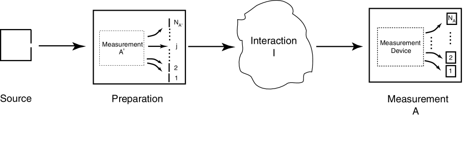
Figure 1: An abstract, idealized experimental-set up. A physical system (such as a silver atom) is emitted from a source, passes a preparation step, and is then subject to a measurement. The preparation is implemented as a measurement, $\mathbf{A}^{\prime}$, which has $N_{A^{\prime}}$ possible outcomes, followed by the selection of those systems which yield some outcome $j$ ($j=1,2,\dots,N_{A^{\prime}}$). The measurement, $\mathbf{A}$, has $N_{A}$ possible outcomes. The measurement detectors are assumed not to absorb the systems that they detect. An interaction, $\mathbf{I}$, may occur as indicated between the preparation and measurement.

We shall only consider set-ups which satisfy particular idealizations. In particular, we shall restrict consideration to measurements that have the following properties:

• Finiteness: the measurements yield a finite number of possible outcomes,

• Distinctness: the possible outcomes of a measurement have distinct values,

• Repetition Consistency: when a measurement is immediately repeated, the same outcome is observed with certainty, and

• Classicality:  the measurements do not involve auxiliary quantum systems.

In addition, we shall assume that interactions have the following properties:

• Identity-preserving: the interactions preserve the identity of the system, and

• Reversible and deterministic: the interactions are reversible and deterministic at the level of the state of the system, and so can be represented as one-to-one maps over state space.

We shall also assume that the background of the system can be adequately modeled within the classical framework insofar as its internal dynamics is concerned. For example, in the case of a system in a background electromagnetic field, the field is assumed to be modeled classically. Similarly, we shall assume that parameters which determine the measurement being performed (the orientation of a Stern-Gerlach apparatus, for instance) are described classically as real-valued numbers. In short, it is assumed that the non-classicality is entirely concentrated in the system and in its interactions with the background and the measurement devices.

Completeness of a Preparation

The essential purpose of the experimental set-up illustrated in Fig. 1 is to allow some property of a physical system to be studied under controlled conditions . Ideally, one would like to prepare the system such that, immediately following the preparation, one has as much knowledge as possible about the degrees of freedom of the state of the system that are relevant to the property under study, and one would like to interact with the system so that only these degrees of freedom are affected. For example, if one wishes to study the spin properties of a system, one would prepare the system so that its spin direction is fixed (in classical physics), or its state is pure (in quantum physics). Similarly, one would allow uniform $\vec{B}$-field interactions since these only affect the spin degrees of freedom of the system, but non-uniform $\vec{B}$-field interactions would be excluded since they couple spin and spatial degrees of freedom, and since spatial degrees of freedom are not under control of the preparation.

Now, ordinarily, we rely upon a particular physical theory to tell us which preparations are maximal with respect to a given measurement in the sense that they provide us with as much control as physically possible over the degrees of freedom of the state of the system that are relevant to predictions concerning the outcomes of the given measurement, and which interactions are compatible with the preparation and measurement in the sense of only affecting the degrees of freedom that are under control of the preparation. However, since our goal is to derive the abstract quantum formalism, where measurements and interactions are treated purely in the abstract, it is necessary to find a way to establish when a preparation is maximal with respect to a given measurement, and when an interaction is compatible with a preparation and measurement, in a correspondingly abstract manner.

To do so, we make use of the fact that, in both classical and quantum physics, a preparation is maximal with respect to a given measurement if and only if the preparation is complete in that it renders the history of the system prior to the preparation irrelevant insofar as predictions concerning the measurement outcomes are concerned. For example, in classical physics, if a preparation places a system in a precisely known state (which is, in principle, possible), one has maximal degree of control over the state, and the results of subsequent measurements performed on the system are independent of the history of the system prior to the preparation, so that the preparation is also complete. The converse is also true.

In quantum physics, one encounters a similar situation. For example, consider an experimental set-up where, in each run, a spin-1/2 system undergoes a preparation by a Stern-Gerlach measurement device, and subsequently undergoes a Stern-Gerlach measurement. From quantum theory, we know that the preparation in this case is maximal with respect to the subsequent Stern-Gerlach measurement, and we also know that the outcome probabilities of the measurement are independent of the pre-preparation history of the spin-1/2 system, so that the preparation is also complete. The converse is also true. More generally, if the preparation of a quantum system is maximal with respect to a given projective measurement, then we know from quantum theory that a system is prepared in a pure state, so that the preparation is also complete with respect to the measurement; and conversely.

Now, most importantly, unlike the notion of maximality, it is straightforward to operationalize the notion of completeness: continuing with the example of the spin-$1/2$ experiment, if one models the data obtained from the measurement in $n$ runs of the experiment using a probabilistic source , one finds that, in the limit of large $n$, the outcome probabilities of the source are independent of arbitrary pre-preparation interactions  with the system.

Using this operationally-defined notion of completeness as a basis, we shall see below that it is possible to give precise expression to the idea that, roughly speaking, a pair of measurements are examining the same property of the system from different perspectives, and that an interaction is only manipulating this particular property of the system.

Definitions

The measurements employed in the abstract set-up are chosen from a measurement set, $\mathcal{A}$. As mentioned previously, it will be assumed that each measurement has the property of finiteness, which we shall now operationalize by saying that, when the measurement is carried out on a system which has been emitted from the source and has undergone arbitrary interactions thereafter, the measurement generates one of a finite number of possible outcomes, a possible outcome being defined as one that has a non-zero probability of occurrence. It will also be assumed that the measurement detectors do not absorb the systems that they detect.

A preparation consists of a measurement that determines to which outcome the incoming system belongs, followed by the selection of the system if the measurement registers a given outcome, and the rejection of the system otherwise. If detectors that do not absorb the detected systems are unavailable, a preparation can instead be implemented using a measurement where one of the detectors is removed.

Consider now an experiment (Fig. 1) in which a system from a source is subject to a preparation consisting of measurement, $\mathbf{A^{\prime}}$, with $N_{A^{\prime}}$ possible outcomes, with outcome $j$ selected ($j=1,\dots,N_{A^{\prime}}$), followed by measurement $\mathbf{A}$ (with $N_{A}$ possible outcomes), without an interaction in the intervening time.

Suppose that the data obtained in $n$ runs of the experiment are modeled by a probabilistic source with $N_{A}$ possible outcomes, whose most likely probabilities (calculated on the basis of the data) are given by $\vec{P}=(P_{1},P_{2},\ldots,P_{N_{A}})$, where $P_{i}$ is the probability of the $i$th outcome $(i=1,2,\dots,N_{A})$  . If, for all $j$, $\vec{P}$ is independent of arbitrary pre-preparation interactions with the system in the limit of large $n$, the preparation will be said to be complete with respect to measurement $\mathbf{A}$. If the completeness condition also holds true when $\mathbf{A}$ and $\mathbf{A}^{\prime}$ are interchanged, then $\mathbf{A}$ and $\mathbf{A}^{\prime}$ will be said to form a measurement pair.

The set of measurements generated by $\mathbf{A}$ forms a measurement set, $\mathcal{A}$, which is defined as the set of all measurements that (i) form a measurement pair with $\mathbf{A}$ and that (ii) are not a composite of other measurements in $\mathcal{A}$. An important corollary of this definition is that two measurement sets are either identical or disjoint.

Interactions that occur after the preparation step are chosen from an interaction set, $\mathcal{I}$, which is defined as follows. Suppose that, in the experiment of Fig. 1, an interaction, $\mathbf{I}$, occurs between the preparation and measurement. If, for all $\mathbf{A},\mathbf{A}^{\prime}\in\mathcal{A}$, the preparation remains complete with respect to the subsequent measurement, then $\mathbf{I}$ will be said to be compatible with $\mathcal{A}$ and the source. The set $\mathcal{I}$ is then defined as the set of all such compatible interactions.

If there are two experimental set-ups, each with a source containing identical copies of the same physical system, with respective disjoint measurement sets, $\mathcal{A}^{(1)}$ and $\mathcal{A}^{(2)}$, then the set-ups will be said to be disjoint. This makes precise the rough notion that the set-ups examine different aspects of the same physical system.

An example

To illustrate the above definitions, consider again the spin-1/2 experiment, where silver atoms emerge from a source (an evaporator), pass through a Stern-Gerlach preparation device, undergo an interaction, and finally undergo a Stern-Gerlach measurement. In this case, the set, $\mathcal{A}$, generated by any Stern-Gerlach measurement consists of all Stern-Gerlach measurements of the form $\mathbf{A}_{\theta,\phi}$, where $(\theta,\phi)$ is the orientation of the Stern-Gerlach device. However, measurements that are composed of two or more Stern-Gerlach measurements are excluded from $\mathcal{A}$.

Consider now an interaction, $\mathbf{I}_{\theta_{B},\phi_{B},t,\Delta t}$, consisting of a uniform $\vec{B}$-field acting during the interval $[t,t+\Delta t]$ in some direction $(\theta_{B},\phi_{B})$. If such an interaction occurs between the preparation and measurement, one finds that the completeness of the preparation with respect to the measurement is preserved; that is, the interaction is compatible with $\mathcal{A}$ and the system. Hence, all interactions in which a uniform magnetic field acts between the preparation and measurement are in the interaction set, $\mathcal{I}$. However, interactions consisting of a non-uniform $\vec{B}$-field do not preserve completeness (viewed from the quantum theoretic model, such interactions couple the spin and position degrees of freedom of the system), and are therefore excluded from $\mathcal{I}$.

Finally, to illustrate the concept of disjoint set-ups, consider a source which emits a system consisting of two distinguishable spin-1/2 particles on each run of an experiment, and consider two set-ups where the first set-up has a measurement set $\mathcal{A}^{(1)}$ consisting of all possible Stern-Gerlach measurements performed on one of the particles, and the second has a measurement set $\mathcal{A}^{(2)}$ consisting of all possible Stern-Gerlach measurements performed on the other particle. In this case, the two measurement sets are disjoint. The set-ups themselves are accordingly said to be disjoint, which precisely expresses the notion that the two set-ups are examining distinct aspects of the same physical system.

II.2 Statement of the Postulates.

Consider the idealized experiment illustrated in Fig. 1 in which a system passes a preparation step that employs a measurement $\mathbf{A}^{\prime}$ in measurement set $\mathcal{A}$, undergoes an interaction, $\mathbf{I}$ in the interaction set $\mathcal{I}$, and is then subject to a measurement, $\mathbf{A}$, in $\mathcal{A}$. The abstract theoretical model that describes this set-up satisfies the following postulates.

1. Measurements

   • Finite and Probabilistic outcomes. When any given measurement $\mathbf{A}\in\mathcal{A}$ is performed, one of $N$ ($N\geq 2$) possible outcomes are observed. The $i$th outcome is obtained with probability $P_{i}$ $(i=1,\dots,N)$, where $P_{i}$ is determined by the preparation, interactions, and measurement.

   • Representation of Measurements. For any given pair of measurements $\mathbf{A},\mathbf{A}^{\prime}\in\mathcal{A}$, there exist interactions $\mathbf{I},\mathbf{I}^{\prime}\in\mathcal{I}$ such that $\mathbf{A}^{\prime}$ can, insofar as probabilities of the outcomes and insofar as the output states of the measurement are concerned, be represented by an arrangement where $\mathbf{I}$ is immediately followed by $\mathbf{A}$ which, in turn, is immediately followed by $\mathbf{I}^{\prime}$.

2. States

   • States. With respect to any given measurement $\mathbf{A}\in\mathcal{A}$, the state, $\mathbf{S}(t)$, of a quantum system at time $t$ is given by $(\vec{P},\vec{\chi})$, where $\vec{P}=(P_{1},P_{2},\dots,P_{N})$ and where $\vec{\chi}=(\chi_{1},\chi_{2},\dots,\chi_{N})$ is a set of $N$ real degrees of freedom.

   • Physical interpretation of the $\chi_{i}$. When measurement $\mathbf{A}\in\mathcal{A}$ is performed on a system in state $\mathbf{S}(t)$ and the outcome $i$ is observed, there are additional outcomes that are objectively realized but unobserved:

     • one of two outcomes, labeled $a$ and $b$, which are obtained with respective probabilities $P_{a|i}=Q^{2}_{a|i}$ and $P_{b|i}=Q^{2}_{b|i}$, where $Q_{a|i}=f(\chi_{i})$ and $Q_{b|i}=\tilde{f}(\chi_{i})$, where $f$ is not a constant function and $f,\tilde{f}$ have range $[-1,1]$, and

     • one of two possible outcomes, with values labeled $+$ and $-$, which is determined by the sign of either $Q_{a|i}$ or $Q_{b|i}$ depending upon whether $a$ or $b$ has been realized.

   • Information Gain. When measurement $\mathbf{A}\in\mathcal{A}$ is performed on a system in any given unknown state $\mathbf{S}(t)$, the amount of Shannon-Jaynes information provided by the observed outcomes and the outcomes $a$ and $b$ about $\mathbf{S}(t)$ in $n$ runs of the experiment is independent of $\mathbf{S}(t)$ in the limit as $n\rightarrow\infty$.

   • Prior probabilities. The prior probability $\Pr(\chi_{i}|\text{I})$, where I is the background knowledge of the experimenter prior to performing the experiment, is uniform for $i=1,\dots,N$.

3. Transformations Any transformation of a prepared physical system, whether active (due to temporal evolution of the system), or passive (a symmetry transformation due to a change of the frame of reference), is represented by a map, $\mathcal{M}$, over the state space, $\mathcal{S}$, of the system.

   • One-to-one. The map $\mathcal{M}$ is one-to-one.

   • Invariance. The map $\mathcal{M}$ is such that, for any state $\mathbf{S}\in\mathcal{S}$, the observed outcome probabilities, $P_{1}^{\prime},P_{2}^{\prime},\dots,P_{N}^{\prime}$, of measurement $\mathbf{A}\in\mathcal{A}$ performed upon a system in state $\mathbf{S}^{\prime}=\mathcal{M}(\mathbf{S})$ are unaffected if, in any representation, $(\vec{P},\vec{\chi})=(P_{i};\chi_{i})$, of the state $\mathbf{S}$ written down with respect to $\mathbf{A}$, any arbitrary real constant, $\chi_{0}$, is added to each of the $\chi_{i}$.

   • Parameterized Transformations. If a physical transformation is continuously dependent upon the real-valued parameter n-tuple $\bm{\pi}$, and is represented by the map $\mathcal{M}_{\bm{\pi}}$, then $\mathcal{M}_{\bm{\pi}}$ is continuously dependent upon $\bm{\pi}$. If the physical transformation is a continuous transformation, then, for some value of $\bm{\pi}$, $\mathcal{M}_{\bm{\pi}}$ reduces to the identity.

   • Temporal Evolution. The map, $\mathcal{M}_{t,\Delta t}$, which represents temporal evolution of a system in a time-independent background during the interval $[t,t+\Delta t]$, is such that any state, $\mathbf{S}$, represented as $(P_{i};\chi_{i})$, of definite energy $E$, whose observable degrees of freedom are time-independent, evolves to $(P_{i}^{\prime};\chi_{i}^{\prime})$, where $P_{i}^{\prime}=P_{i}$ and $\chi_{i}^{\prime}=\chi_{i}-E\Delta t/\alpha$, where $\alpha$ is a non-zero constant with the dimensions of action.

4. Consistency The posterior probability distributions over $\mathcal{S}$ that result from the following two processes coincide in the limit as $n\rightarrow\infty$:

   • inferring a posterior over $\mathcal{S}$ based upon the objectively realized outcomes when the measurement $\mathbf{A}\in\mathcal{A}$ is performed upon $n$ copies of a system in state $\mathbf{S}$, and then transforming the posterior using $\mathcal{M}$, or

   • inferring a posterior over $\mathcal{S}$ based upon the objectively realized outcomes when the measurement $\mathbf{A}\in\mathcal{A}$ is performed upon $n$ copies of a system in state $\mathcal{M}(\mathbf{S})$,

The above postulates, together with the Average-Value Correspondence Principle (AVCP), which will be given in Paper II, suffice to determine the form of the abstract quantum model for the abstract set-up. From Postulates 1.1 and 1.3, it follows that, when any measurement in $\mathcal{A}$ is performed on the system, one of $N$ possible outcomes is observed. Accordingly, we shall denote the abstract quantum model of such a set-up by $\mathbf{q}(N)$.

Finally, we shall need Postulates 5, below, in order to obtain a rule, which we shall refer to as the composite systems rule, for relating the quantum model of a composite system to the quantum models of its component systems:

1. Composite Systems Suppose that a system admits a quantum model with respect to the measurement set $\mathcal{A}^{(1)}$ whose measurements have $N^{(1)}$ possible observable outcomes, and admits a quantum model with respect to measurement set $\mathcal{A}^{(2)}$ whose measurements have $N^{(2)}$ possible observable outcomes, where the sets $\mathcal{A}^{(1)}$ and $\mathcal{A}^{(2)}$ are disjoint.

   Consider the quantum model of the system with respect to the measurement set $\mathcal{A}=\mathcal{A}^{(1)}\times\mathcal{A}^{(2)}$ that contains all possible composite measurements consisting of a measurement from $\mathcal{A}^{(1)}$ and a measurement from $\mathcal{A}^{(2)}$. If the states of the sub-systems are represented as $(P_{i}^{(1)};\chi_{i}^{(1)})$ $(i=1,2,\dots,N^{(1)})$ and $(P_{j}^{(2)};\chi_{j}^{(2)})$ $(j=1,2,\dots,N^{(2)})$, respectively, then the state of the composite system can be represented as $(P_{ij};\chi_{ij})$, where $P_{ij}=P_{i}^{(1)}P_{j}^{(2)}$ and $\chi_{ij}=\chi_{i}^{(1)}+\chi_{j}^{(2)}$.

III Overview of the Postulates

Many of the postulates described above can be seen to follow from the quantum formalism, which provides some understanding of these postulates. Accordingly, we shall first point out the relations between these postulates and the quantum formalism. We shall then describe how the postulates can be physically understood.

III.1 Postulates that follow from quantum theory

Of the postulates enumerated above, all apart from Postulates 2.2, 2.3, 2.4 and 4 can be seen to follow from the quantum formalism.

Consider the quantum theoretical model of the abstract experimental set-up. Since the measurements in measurement set $\mathcal{A}$ yield one of $N$ possible distinct observable outcomes, it follows that the state space of the quantum model is $N$-dimensional. Furthermore, since a preparation (implemented using a measurement $\mathbf{A}^{\prime}\in\mathcal{A}$) is complete with respect to a measurement $\mathbf{A}\in\mathcal{A}$, it follows that the system immediately following the preparation step is in a pure state, $\textsf{v}\in\mathbb{C}^{N}$.

According to the quantum formalism, measurement $\mathbf{A}$ can be represented by a Hermitian operator, A. With respect to this measurement, the $i$th component of v can be written as $P_{i}e^{i\phi_{i}}$, where $P_{i}$ is the outcome probability of outcome $i$, so that the state can be represented as

$$\textsf{v}=(P_{1},\dots,P_{N};\phi_{1},\dots,\phi_{N}),$$ (1)

or $(P_{i};\phi_{i})$ for short, which yields Postulates 1.1 and 2.1.

In the quantum model, it is assumed that physical transformations are represented by unitary or antiunitary transformations of state space. Unitary and antiunitary transformations are one-to-one maps, which gives Postulates 3 and 3.1. To show Postulate 3.2, consider the transformation of $\textsf{v}e^{-i\phi_{0}}$ by the unitary operator U. The transformed vector is

$$\textsf{v}^{\prime}=e^{-i\phi_{0}}\textsf{U}\textsf{v}.$$ (2)

However, the outcome probabilities of any measurement performed on the system in state $\textsf{v}^{\prime}$ are independent of the overall phase of $\textsf{v}^{\prime}$. Therefore, these outcome probabilities are unaffected if an arbitrary $\phi_{0}\in\mathbb{R}$ is added to the $\phi_{i}$, where v is represented as in Eq. (1).

Postulate 3.3 is obtained in two parts. First, if a physical transformation depends continuously upon a set of real-valued parameters, then it is represented by a unitary or antiunitary transformation whose degrees of freedom also continuously depend upon these parameters. Second, continuous transformations are represented by unitary transformations. If a unitary transformation is a continuous function of a set of real-valued parameters, then it is possible that, for some values of these parameters, the unitary transformation reduces to the identity.

From the unitary operator $\textsf{U}_{t}(\Delta t)=\exp(-i\textsf{H}_{t}\Delta t/\hbar)$ for the evolution of a system during the interval $[t,t+\Delta t]$ in a time-independent background, where $\textsf{H}_{t}$ is the Hamiltonian operator at time $t$, it follows that a state v which is an eigenstate of $\textsf{H}_{t}$ evolves into

$$\textsf{v}^{\prime}=e^{-iE\Delta t/\hbar}\textsf{v},$$ (3)

where $E$ is the energy of the state. In the representation of Eq. (1), the state $(P_{i};\phi_{i})$ evolves to $(P_{i};\phi_{i}-E\Delta t/\hbar)$, and, since v and $\textsf{v}^{\prime}$ differ only by an overall phase, they are observationally indistinguishable, which gives Postulate 3.4.

To show Postulate 1.2, suppose that one wishes to represent $\mathbf{A}^{\prime}$ in terms of measurement $\mathbf{A}$. Consider an arrangement consisting of a unitary transformation U immediately followed by measurement $\mathbf{A}$, followed immediately, in turn, by $\textsf{U}^{\dagger}$. Suppose that measurements $\mathbf{A}$ and $\mathbf{A}^{\prime}$ are represented by the operators A and $\textsf{A}^{\prime}$, respectively, where $\textsf{A}\textsf{v}_{i}=a_{i}\textsf{v}_{i}$ and $\textsf{A}^{\prime}\textsf{v}^{\prime}_{i}=a_{i}^{\prime}\textsf{v}^{\prime}_{i}$. Then, if we choose

$$\textsf{U}=\sum_{i}\textsf{v}_{i}\textsf{v}^{\prime\dagger}_{i},$$ (4)

this arrangement behaves precisely the same as measurement $\mathbf{A}^{\prime}$ insofar as the probabilities of the observed outcomes and insofar as the corresponding output states are concerned. To see this, note that, if the input state to the arrangement is $\sum_{i}c_{i}^{\prime}\textsf{v}_{i}^{\prime}$ (the $c_{i}^{\prime}$ being complex constants, such that $\sum_{i}|c_{i}^{\prime}|^{2}=1$) the state $\textsf{U}\sum_{i}c_{i}^{\prime}\textsf{v}_{i}^{\prime}=\sum_{i}c_{i}^{\prime}\textsf{v}_{i}$, and therefore measurement $\mathbf{A}$ yields outcome $i$ with probability $|c_{i}^{\prime}|^{2}$ and yields corresponding state $\textsf{v}_{i}$ up to an irrelevant overall phase. The final output state of the arrangement is therefore $\textsf{U}^{\dagger}\textsf{v}_{i}=\textsf{v}_{i}^{\prime}$. Hence, the arrangement behaves precisely as would measurement $\mathbf{A}^{\prime}$ performed directly on a system in state $\textsf{v}^{\prime}$ in respect of the probabilities of observed outcomes $1,2,\dots,N$ and in respect of the output states.

Finally, by considering the tensor product $\textsf{v}=\textsf{v}^{(1)}\otimes\textsf{v}^{(2)}$ where $\textsf{v}^{(1)}\in\mathbb{C}^{N_{1}}$ and $\textsf{v}^{(2)}\in\mathbb{C}^{N_{2}}$ are the states of two sub-systems, and $\textsf{v}\in\mathbb{C}^{N}$, with $N=N_{1}N_{2}$, is the state of the composite system, one finds that Postulate 5 follows at once.

III.2 Physical Comprehensibility of the postulates.

When formulating the postulates, our goal has been to maximize their physical comprehensibility. For the purposes of discussion, it is helpful to distinguish two levels of physical comprehensibility. First, at the minimum, a comprehensible postulate is one that can be transparently understood as a simple assertion about the physical world. If this is the case, we shall say that the postulate has the property of transparency. Second, a postulate has an additional level of comprehensibility if it can also be traced to well-established experimental facts and physical ideas or principles (traceability).

To illustrate these ideas, consider the example of Einstein’s postulate of the constancy of the speed of light. The postulate can be transparently understood as the simple assertion that measurements of the speed of light in different inertial frames will yield the same result. In addition, the postulate can also be understood as a direct generalization of the well-established results of the Michelson-Morley experiment, the generalization being achieved by an appeal to the general principle of the uniformity of nature. Hence, the postulate is both transparent and traceable.

Since the assumptions underlying classical physics are transparent and traceable to well-established experimental facts and theoretical ideas, and since these assumptions remain fundamental to the way in which we conceptualize the physical world, we attempt to preserve them as far as possible in the face of quantum phenomena. Accordingly, we draw the majority of the postulates from classical physics, either by taking fundamental features of the theoretical framework of classical physics and modifying these, if necessary, in light of experimental facts that are characteristic of quantum phenomena, or by transposing particular features of the classical models of physical systems into the quantum realm via a classical–quantum correspondence argument. Furthermore, in our treatment of information, we use the standard inferential methods of probability theory, and employ the conceptually and mathematically well-established framework of Shannon information theory. The remaining assumptions, which have no obvious classical counterparts, are based on experimental facts that are characteristic of quantum phenomena but have no classical analog, or are based on novel theoretical ideas and principles.

In our discussion below, we shall divide the postulates into (i) postulates that are adopted from classical physics, or are modified therefrom in light of experimental facts characteristic of quantum phenomena, (ii) postulates that are obtained through a classical-quantum correspondence argument, and (iii) novel postulates with no classical counterparts.

Postulates adopted from classical physics.

A classical model of a physical system is based upon the partitioning, time and states background assumptions given earlier, and these are adopted unchanged in the abstract quantum model. The classical model additionally makes the following additional key assumptions:

1. Measurements.

   • Operational Determinacy. The outcome of a measurement performed on the system is determined by experimentally-controllable variables.

   • Continuum. The values of the possible outcomes of a measurement form a real-valued continuum.

2. States.

   • Determinacy. The state of the system and a theoretical description of a measurement that is performed on the system determine the measurement outcome.

3. Transformations.

   • Mappings. Physical transformations of the system, either due to temporal evolution or due to a passive change of frame of reference, are represented by mappings over the space of states.

   • One-to-one. The mappings are one-to-one.

   • Continuity. If a map represents a physical transformation that depends continuously upon a real-valued set of parameters, then the map is continuously dependent upon these parameters.

   • Continuous transformations. If a map represents a continuous transformation (such as temporal evolution) that depends continuously upon a set of real-valued parameters, then, for some value of these parameters, the map reduces to the identity.

We remark that the measurements mentioned in A1–2 are idealized, fundamental measurements, such as measurements of the position of a particle, which, in the framework of classical physics, are assumed to yield a continuum of possible outcomes . Similarly, although fundamental measurements of a physical quantity in a particular situation (such as the frequency of a bound membrane) may take a discrete number of possible values, it is assumed that the discreteness arises through the particular boundary conditions that are applicable, rather than being an intrinsic feature of the measurements themselves.

We also remark that, in C0-C3, it is assumed that physical transformations of a physical system are deterministic and reversible, which prevents the description of irreversible or indeterministic transformations within the classical framework at a fundamental level.

First, we consider those postulates which adopt classical assumptions unchanged. Postulates 3 and 3.1 correspond, respectively, to assumptions C0 and C1, while Postulate 3.3 is a combination of assumptions C2 and C3.

Second, in light of the results of experiments involving quantum systems (such as Stern-Gerlach measurements on silver atoms), it is reasonable to modify assumptions A1, A2 and B1 as follows:

• Probabilistic operational determinacy. The data obtained when a measurement is performed on the system are best modeled by a probabilistic source whose outcome probabilities are determined by experimentally-controllable variables.

• Finiteness. A measurement performed on a system has a finite number of possible outcomes.

• Probabilistic determinacy. The state of the system and a theoretical description of a measurement that is performed on the system only probabilistically determine the measurement outcome.

We emphasize that, although these modifications are reasonable, they are not the only possibilities consistent with the experimental facts. For example, the probabilistic operational determinacy that one finds empirically can be accommodated in at least two ways. First, one can assume that the state of the system does, in fact, determine the outcome of a measurement performed upon the system, but that one cannot, for some reason, control all of the relevant degrees of freedom of state. Second, one can assume that the degrees of freedom of the state only determine the probability that a measurement yields a particular value. In this instance, we have taken the latter option.

These modified assumptions are contained within Postulates 1.1 and 2.1. Specifically, Postulate 1.1 contains assumption A1^′ and A2^′, while Postulate 2.1 incorporates assumption B1^′.

Postulates obtained through classical-quantum correspondence.

A general guiding principle in building up a quantum model of a physical system is that, in an appropriate limit, the predictions of the quantum model of the system stand in some one-to-one correspondence with those of a classical model of the system. By establishing such a correspondence between the quantum and classical models of a particle, we shall transpose several elementary properties of the classical model across to the quantum model and then, by generalization, to the abstract quantum model, $\mathbf{q}(N)$.

Consider an experiment in which a position measurement is used to prepare a particle at time $t_{0}$, and a position measurement is subsequently performed at time $t_{1}$, during which interval a potential $V(\vec{r},t)$ is assumed to act. When such an experiment is actually performed, one necessarily uses position measurements with a finite number of possible outcomes. In this case, the experimental results (where, for instance, an electron passes through a sub-micron aperture, is subject to electric-field interactions, and is subsequently detected on a screen) support the conclusion that, if these coarse position measurements are of sufficiently high spatial resolution, the preparation is, to a very good approximation, complete with respect to the subsequent measurement.

Suppose, then, that a coarse position measurement with $N$ possible outcomes is used to implement both the preparation and measurement steps, and further let us suppose that the coarse measurement is such that the probability that a detection is obtained in any run of the experiment is very close to unity. Further, let us suppose that the coarse measurement is of sufficient resolution that the preparation can be regarded as being complete with respect to the measurement. Then we can form a quantum model, which we shall denote $\mathbf{q}^{*}(N)$, within the framework of the abstract quantum model $\mathbf{q}(N)$, which approximately describes the experiment after time $t_{0}$.

By Postulate 1.1 and the assumption B1^′ above, the state, $\mathbf{S}(t_{1})$, of the system immediately prior to the coarse position measurement determines the probability n-tuple, $\vec{P}(t_{1})=(P_{1},\dots,P_{N})$, where $P_{i}$ is the probability of detection at the $i$th detector, which characterises the data obtained from the coarse position measurement.

If the above experiment is repeated, except that the coarse position measurement is delayed until time $t_{2}$, then $\mathbf{S}(t_{1})$, together with a theoretical representation of any interaction in the interval $[t_{1},t_{2}]$, must (by assumption B1^′) enable the prediction of the probability n-tuple $\vec{P}(t_{2})$ that describes the coarse position measurement data obtained at time $t_{2}$. To determine what additional degrees of freedom the state $\mathbf{S}(t_{1})$ must contain in order to make this prediction possible, consider the classical limit.

Suppose that $m$ is increased towards values characteristic of macroscopic bodies. Under the assumption made above, the preparation is complete with respect to the measurement, so that the system continues to be well-described by the model $\mathbf{q}(N)$ even in this classical limit. However, as $m$ tends towards macroscopic values, it is reasonable to expect that the system will increasingly behave in accordance with its classical model between times $t_{1}$ and $t_{2}$. That is, in this classical limit, we expect that $\vec{P}(t_{2})$, which is determined in the quantum model in terms of $\vec{P}(t_{1})$ and the other degrees of freedom in $\mathbf{S}(t_{1})$, will coincide with the n-tuple $\vec{P}^{(\text{CM})}(t_{2})$ that is predicted by a classical model of a particle of mass $m$ moving in the same potential.

The relevant classical model in this situation is a particle ensemble model. For such an ensemble model, one can choose to describe an ensemble for the case of given total energy by means of a probability density function over phase space, and to describe the evolution of this function using Newton’s equations of motion. Alternatively, one can employ the Hamilton-Jacobi model, which is physically equivalent. We choose the latter since it is more easily described on a discrete spatial lattice.

In the Hamilton-Jacobi model, the state of the ensemble is given by $(P(\vec{r},t),S(\vec{r},t))$, which satisfies the Hamilton-Jacobi equations,

$$\begin{gathered}\frac{\partial P}{\partial t}+\nabla.\left(\frac{1}{m}P\,\nabla S\right)=0\\ \frac{1}{2m}\left(\nabla S\right)^{2}+V(\vec{r},t)=-\frac{\partial S}{\partial t}.\end{gathered}$$ (5)

In the case of coarse position measurements with $N$ possible outcomes, we shall use the discretized form of the Hamilton-Jacobi state, $(\vec{P}^{(\text{CM})};S_{i})$, with $i=1,\dots,N$, and with $\vec{P}^{(\text{CM})}=(P_{1}^{(\text{CM})},\dots,P_{N}^{(\text{CM})})$, where $P_{i}^{(\text{CM})}$ is the probability that the position measurement yields a detection at the $i$th measurement location, and $S_{i}$ is the classical action at the $i$th measurement location.

In order that the predictions of the quantum and classical models agree in the classical limit, the quantum state $\mathbf{S}(t)$ ($t>t_{0}$) must contain degrees of freedom which encode $N$ quantities, which we shall denote $S^{(\text{QM})}_{1},\dots,S^{(\text{QM})}_{N}$, which, in the classical limit, are equal to the $S_{i}$. Equivalently, we shall assume that $\mathbf{S}$ contains $N$ dimensionless real quantities, $\chi_{1},\dots,\chi_{N}$, such that $S^{(\text{QM})}_{i}=\alpha\chi_{i}$, where $\alpha$ is a constant with dimensions of action.

From the above discussion, in the model $\mathbf{q}^{*}(N)$, the state, $\mathbf{S}$, is given by $(\vec{P},\vec{\chi})$, where $\vec{\chi}=(\chi_{1},\dots,\chi_{N})$. Postulate 2.1 directly generalizes this statement to the abstract model $\mathbf{q}(N)$.

We now observe that the Hamilton-Jacobi model has the following properties, which can be readily verified from Eq. (5):

• Invariance. The evolution of the state $(\vec{P}^{(\text{CM})}(t_{1});S_{i}(t_{1}))$ to the state $(\vec{P}^{(\text{CM})}(t_{2});S_{i}(t_{2}))$ is such that $\vec{P}^{(\text{CM})}(t_{2})$ is unchanged if an arbitrary real constant, $S_{0}$, is added to each of the $S_{i}(t_{1})$.

• Temporal Evolution. In a time-independent background, a state, $(\vec{P}^{(\text{CM})}(t);S_{i}(t))$ whose observable degrees of freedom are time-independent, evolves in time $\Delta t$ to the state $(\vec{P}^{(\text{CM})}(t);S_{i}(t)-E\Delta t)$, where $E$ is the total energy of the system.

• Composite Systems. If, with respect to position measurements along the $x$ and $y$ axes, the Hamilton-Jacobi state of a particle is $(P^{CM(x)}_{i},S^{(x)}_{i})$ and $(P^{CM(y)}_{j},S^{(y)}_{j})$, respectively, then, with respect to $xy$-position measurements, its state is $(P^{CM(xy)}_{ij},S^{(xy)}_{ij})=(P^{CM(x)}_{i}P^{CM(y)}_{j},S^{(x)}_{i}+S^{(y)}_{j})$

Furthermore, from the first property, since the zero-value of the $S_{i}$ is conventional and therefore has no physical correlate, the prior probability $\Pr(S_{i}|\text{I})$ must be invariant under arbitrary changes of the zero-value of the $S_{i}$, where $I$ represents the state of knowledge of the experimenter prior to performing a measurement on the system. The uniform prior is the only prior that has this invariance property. Therefore, the prior $\Pr(S_{i}|\text{I})$ is uniform, which we shall list as a fourth property:

• Prior Probabilities. The prior $\Pr(S_{i}|\text{I})$ is uniform ($i=1,2,\dots,N$), where $I$ represents the state of knowledge of the experimenter prior to performing a measurement on the system.

On the assumption of the above correspondence between the Hamilton-Jacobi model and the model $\mathbf{q}^{*}(N)$, it is now possible to transpose these properties to the model $\mathbf{q}^{*}(N)$ in the classical limit.

For example, Postulate 2.4 is obtained as follows. First, by using the relation $\Pr(S_{i}|\text{I})|dS_{i}|=\Pr(\chi_{i}|\text{I})|d\chi_{i}|$, it follows that

$$\Pr(\chi_{i}|\text{I})\left|dS_{i}/d\chi_{i}\right|^{-1}=\Pr(S_{i}|\text{I}).$$ (6)

Then, using the correspondence relation that $S_{i}=\alpha\chi_{i}$ in the classical limit, and noting that $\Pr(S_{i}|\text{I})$ is uniform (property 4, above), we conclude that, in the classical limit, the model $\mathbf{q}^{*}(N)$ satisfies the condition that $\Pr(\chi_{i}|\text{I})$ is a constant. Second, the assumption is made that this condition holds for the model $\mathbf{q}^{*}(N)$ not only in the classical limit but also for microscopic values of $m$ and, even more generally, that it holds for the abstract quantum model $\mathbf{q}(N)$.

Postulates 3.2, 3.4 and 5 are obtained in a similar manner by using the above correspondence, $S_{i}=\alpha\chi_{i}$, to transpose the first three properties to the model $\mathbf{q}^{*}(N)$ in the classical limit, and then making the assumption that the transposed properties hold more generally for the abstract quantum model $\mathbf{q}(N)$.

Novel Postulates

Below, we shall describe the four novel postulates, namely Postulates 1.2, 2.2, 2.3 and 4.

Postulate 1.2: Representation of Measurements.

Consider an experiment in which Stern-Gerlach preparations and measurements are performed upon silver atoms, and where the set $\mathcal{A}$ consists of the elements $\mathbf{A}_{\theta,\phi}$ representing Stern-Gerlach measurements in the direction $(\theta,\phi)$. In this experiment, if an interaction consisting of a uniform magnetic field acts between the preparation and measurement, one finds that both the probabilities of the observed outcomes are the same as would be obtained if a different measurement had been done with the solenoid absent.

Using this observation, one finds that it is possible to implement the measurement $\mathbf{A}_{\theta,\phi}$ using any given measurement $\tilde{\mathbf{A}}\in\mathcal{A}$ if followed immediately before and after by suitable interactions. The implementation behaves precisely as $\mathbf{A}_{\theta,\phi}$ insofar as the probabilities of observable outcomes $1$ and $2$, and the corresponding output states, are concerned. Postulate 1.2 can be regarded as a plausible generalization of this observation.

Postulate 2.2: Physical interpretation of the $\chi_{i}$.

According to Postulate 2.1, the state $S(t)$, written with respect to some measurement $\mathbf{A}\in\mathcal{A}$, consists of the pair $(\vec{P},\vec{\chi})$, where $\vec{P}$ contains the probabilities of the observed outcomes, and $\vec{\chi}$ is an ordered set of real-valued degrees of freedom. Hence, the state consists of a mixture of probabilities and degrees of freedom unconnected to probabilities. Postulate 2.2 is motivated by the aesthetical desideratum that a quantum state consist, as far as possible, of probabilities of events, rather than being such a mixture.

Accordingly, we postulate that $\chi_{i}$ encodes the probabilities of some events, labeled $a$ and $b$. Hence, when measurement $\mathbf{A}$ is performed on the system, one of $2N$ possible outcomes is obtained, with probabilities determined by the state of the system. Since, by Postulate 1.1, the probabilities of the observed outcomes of measurement $\mathbf{A}$ are determined by the $P_{i}$, we are forced to postulate that, for some reason to be investigated later, the outcomes $a$ and $b$ are not observed by the experimenter.

Now, we make the reasonable assumption that the abstract quantum framework being developed is capable of modeling the behavior of a photon when subject to polarization measurements, and that this model will agree with the predictions of electromagnetism under a particle interpretation. Now, an electromagnetic plane wave of constant amplitude moving along the $+z$-direction is described by the vector-valued function $\vec{E}=E_{0}(\cos\theta\,\vec{i}+\sin\theta\,\vec{j})$, and the information about the polarization of the wave is contained in $(\cos\theta,\sin\theta)$ with respect to polarization measurements in the $xy$-plane. In the particle interpretation, the probability that a photon will pass through a polarizer whose axis points along the $x$-axis or $y$-axis is given by $\cos^{2}\theta$ or $\sin^{2}\theta$, respectively. The key feature which we wish to abstract from this example is that, since the map from $(\cos\theta,\sin\theta)$ (the ‘state-level’) to $(\cos^{2}\theta,\sin^{2}\theta)$ (the ‘probability-level’) is many-to-one, the computed probabilities are not the fundamental quantities when describing the state of the photon. Rather, the more fundamental quantities are $\cos\theta$ and $\sin\theta$, which we can regard as square roots of probability in the range $[-1,1]$, which are squared to obtain probabilities.

To incorporate this two-layered feature into the abstract quantum model, we assume that, following the realization of outcome $a$ or $b$, one of two outcomes, labeled $+$ and $-$, is obtained. This ensures that one binary-valued degree of freedom is associated with each of the $2N$ possible probabilistically-determined outcomes. Furthermore, we assume that the value of $\chi_{i}$ determines whether $+$ or $-$ is obtained via the sign of either $Q_{a|i}$ or $Q_{b|i}$, depending upon whether $a$ or $b$ was obtained, where $P_{a|i}=Q^{2}_{a|i}$ and $P_{b|i}=Q^{2}_{b|i}$. In summary, the quantum state consists of the $N$ probabilities $P_{1},\dots,P_{N}$ and the $2N$ quantities $Q_{a|1},Q_{b|1},\dots,Q_{a|N},Q_{b|N}$ which encode the probabilities $P_{a|1},P_{b|1},\dots,P_{a|N},P_{b|N}$ and encode the values of the $2N$ binary-valued degrees of freedom.

In Sec. V.1, we sketch some ideas which help to provide a better physical understanding of this postulate.

Postulate 2.3: Principle of Information Gain.

Postulate 2.3 asserts that, in the arrangement of Fig. 1, if measurement $\mathbf{A}\in\mathcal{A}$ is performed on a system in any unknown state $\mathbf{S}(t)$, then, in $n$ runs of the experiment, the amount of information provided by the probabilistically-determined outcomes (namely, one of $1,\dots,N$, followed by either $a$ or $b$) about $\mathbf{S}(t)$ is independent of $\mathbf{S}(t)$ in the limit as $n\rightarrow\infty$. This postulate can be understood physically as follows.

Suppose that, in trial $1$ of $n$ runs of an experiment, a measurement $\mathbf{A}$ is performed on a system in state $\mathbf{S}(t)$, and suppose that trial $2$ is identical to trial $1$ except that measurement $\mathbf{A}^{\prime}$ is performed instead of $\mathbf{A}$. Now, by Postulate 1.2, trial $2$ is equivalent (insofar as the probabilities of the probabilistically-determined outcomes are concerned) to trial $2^{\prime}$ consisting of $n$ runs of an experiment where a system in state $\mathbf{S}(t)$ is sent through an arrangement consisting of a suitable physical interaction with the system, represented by map $\mathcal{M}$ (Postulate 3), followed by measurement $\mathbf{A}$, followed by another physical interaction.

The data obtained in trials $1$ and $2$ provides information (via the Shannon-Jaynes entropy functional, as we shall later detail) about $S(t)$. Furthermore, since the data obtained in trials $2$ and $2^{\prime}$ is statistically identical (as ensured by Postulate 1.2), the amount of information obtained about $S(t)$ in trial $2$ is asymptotically equal to the amount of information obtained about $S^{\prime}(t)=\mathcal{M}\left(S(t)\right)$ in trial $2^{\prime}$

Now, suppose that, in one of the two trials $1$ and $2$, the data obtained yields more information about the state $S(t)$ than in the other trial. This implies that, in the trials $1$ and $2$, one of the two measurements $\mathbf{A}$ and $\mathbf{A}^{\prime}$ is privileged compared to the other insofar as the amount of information that it yields about $\mathbf{S}(t)$. Although this possibility cannot be ruled out a priori, we make the intuitively plausible assertion that, although these different measurements provide different perspectives on the system, these perspectives are not informationally privileged. Postulate 2.3 ensures that the amount of information obtained in trials $1$ and $2^{\prime}$ is asymptotically equal and, therefore, that the amount obtained in trials $1$ and $2$ is equal. That is, Postulate 2.3 can be understood as arising from the requirement that no measurement in the measurement set provides an informationally privileged perspective on the system.

In order to quantify the amount of information gained, the Shannon-Jaynes entropy functional (also known as the relative entropy) has been used (see Eq. (12)), which is the continuum generalization of the Shannon entropy . Although other discrete information measures, such as the Rényi or Tsallis entropies Renyi65 ; Tsallis88 , have been proposed, the Shannon-Jaynes entropy is preferred here since the Shannon entropy has the clearest axiomatic basis (being derivable from a set of intuitively reasonable postulates Shannon48 ; Khinchen57a ; Faddeev57 ) and has strong indirect support through applications in communication theory and through the many successes of the maximum entropy method (see Jaynes57a ; Jaynes57b , for example), of which it forms the basis.

In Sec. V.1, we shall develop a better understanding of this postulate and describe some of its interesting consequences.

Postulate 4: Consistency.

A fundamental requirement of a theoretical model is that it be internally consistent. That is, if it is possible to make a particular prediction via two distinct calculational pathways, the predictions obtained must agree.

Postulate 4 considers the particular situation where one attempts to calculate a posterior probability distribution over state space on the basis of the objectively realized outcomes (see Postulate 2.2) in $n$ runs of an experiment in which a measurement, $\mathbf{A}$, is performed on a system.

In particular, one can arrive at the posterior, $p^{\prime}(\mathbf{S})$, via two calculational pathways:

$$\begin{CD}\mathbf{S}@>{\text{Map~{}$\mathcal{M}$}}>{}>\mathbf{S}^{\prime}=\mathcal{M}(\mathbf{S})\\ @V{\text{Measurement~{}$\mathbf{A}$}}V{}V@V{}V{\text{Measurement~{}$\mathbf{A}$}}V\\ p(\mathbf{S})@>{\text{Map~{}$\mathcal{M}^{*}$}}>{}>p^{\prime}(\mathbf{S})\end{CD}$$

In the first route, in a given run of the experiment, state $\mathbf{S}$ is first transformed to state $\mathbf{S}^{\prime}=\mathcal{M}(\mathbf{S})$, and then one performs measurement $\mathbf{A}$ on the system. On the basis of the data obtained in $n$ runs, one then calculates a posterior probability distribution over state space. In the second route, in a given run, one first performs the measurement on the system in state $\mathbf{S}$. On the basis of the data obtained in $n$ runs, one calculates a posterior, $p(\mathbf{S})$, over state space, and then transforms this posterior using the map $\mathcal{M}^{*}$, which is determined by $\mathcal{M}$.

Although these two calculational routes cannot be expected to agree for finite $n$ owing to statistical fluctuations, consistency requires that they agree (so that the above diagram commutes) in the limit as $n\rightarrow\infty$.

IV Deduction of the quantum formalism

In this section, we shall use the postulates described above to derive the explicit form of the abstract quantum model $\mathbf{q}(N)$, apart from the representation of temporal evolution (which is derived in Paper II). We shall also derive the composite systems rule which allows the abstract quantum model of a composite system to be related to the abstract quantum models of its component systems.

The derivation will proceed as follows. First, in Sec. IV.1, we shall explore the consequences of Postulate 2.3, the principle of information gain. We shall find that, if an information gain condition applies to a probabilistic source with probability n-tuple $\vec{P}=(P_{1},P_{2},\dots,P_{M})$ ($M\geq 2$), then, if $\vec{P}$ is represented as a unit vector, $\vec{Q}=(\sqrt{P}_{1},\sqrt{P}_{2},\dots,\sqrt{P}_{M})$, in a real ‘square-root of probability’ space (or $Q$-space), the prior $\Pr(\vec{Q}|\text{I})$ is uniform over the positive orthant of the unit hypersphere in this space.

Second, following Postulates 1.1, 2.1, and 2.2, we shall represent the state of a system, $\mathbf{S}(t)$, in a $2N$-dimensional $Q$-space, $Q^{2N}$. We shall then use Postulate 2.4 to determine the form of the function $f$ that is introduced in the postulates.

Third, in Sec. IV.2, we shall use Postulates 3, 3.1, 3.2, 3.3 and 4 in order to obtain a representation of physical transformations of a system. We shall find that such transformations can be represented by a subset of the orthogonal transformations of the unit hypersphere in $Q^{2N}$. We shall then show that these transformations can, equivalently, be represented by the set of unitary and antiunitary transformations of a suitably-defined $N$-dimensional complex vector space.

Fourth, in Sec. IV.3, we shall draw upon Postulate 1.2 in order to obtain a representation of measurements on a system.

Fifth, in Sec. IV.4, we shall use Postulate 5 to obtain a rule, the composite system rule, which determines the state of a composite system in terms of the states of its sub-systems.

IV.1 Probabilistic Sources and Information Gain

By postulates 1.1, 2.1 and 2.2, the measurement $\mathbf{A}$ on the system in state $\mathbf{S}(t)$ can, with respect to the outcomes labeled $i$ and $a$ or $b$, be modeled as the interrogation of a $2N$-outcome probabilistic source with probability n-tuple

$$\mathbf{P}=(P_{1}P_{a|1},P_{1}P_{b|1},\dots,P_{N}P_{a|N},P_{N}P_{b|N}).$$ (7)

From Postulate 2.2, $f$ has range $[-1,1]$, so that all possible values of $\mathbf{P}$ can be obtained by varying the state $S(t)$. From Postulate 2.3, it therefore follows that, when this probabilistic source with any given $\mathbf{P}$ is interrogated $n$ times, the amount of Shannon-Jaynes information obtained about $\mathbf{P}$ by an experimenter who does not know the value of $\mathbf{P}$ is independent of $\mathbf{P}$ in the limit as $n\rightarrow\infty$. In order to implement this condition, we shall begin by examining the process by which information is gained about a probabilistic source.

Information gain from a probabilistic source.

Consider an experiment in which an $M$-outcome probabilistic source, with probability n-tuple $\vec{P}=(P_{1},P_{2},\ldots,P_{M})$, is interrogated $n$ times, yielding the data string, $D_{n}=a_{1}a_{2}\ldots a_{n}$, of length $n$, where $a_{r}$ represents the value of the $r$th outcome ($r=1,\dots,n$).

Let us suppose that an experimenter knows that the data is obtained from a probabilistic source, but does not the value of $\vec{P}$. Since the experimenter knows that the data is generated by a probabilistic source, the order of the $a_{r}$ is irrelevant, the only relevant data being the number of instances, $m_{i}$ of each outcome, $i$ ($i=1,\dots,M$), which can be encoded in the data n-tuple $\vec{m}=(m_{1},m_{2},\ldots,m_{M})$, or, equivalently, in the pair $(\vec{f},n)$, where $\vec{f}=\vec{m}/n$ is the frequency n-tuple.

The experimenter’s knowledge about $\vec{P}$ prior to the experiment can be expressed as the prior probability density function $\Pr(\vec{P}|\text{I})$, where I symbolizes the knowledge that the experimenter possesses prior to performing the interrogations.

After obtaining the data $(\vec{f},n)$, the experimenter’s state of knowledge about $\vec{P}$ is represented by the posterior probability density function, $\Pr(\vec{P}|\vec{f},n,\text{I})$. The posterior can be related to the prior using Bayes’ theorem,

$$\Pr(\vec{P}|\vec{f},n,\text{I})=\frac{\Pr(\vec{f}|\vec{P},n,\text{I})\Pr(\vec{P}|n,\text{I})}{\Pr(\vec{f}|n,\text{I})},$$ (8)

where the function $\Pr(\vec{f}|\vec{P},n,\text{I})$, known as the likelihood, is given by

$$\Pr(\vec{f}|\vec{P},n,\text{I})=\frac{n!}{(nf_{1})!\dots(nf_{M})!}P_{1}^{nf_{1}}\dots P_{M}^{nf_{M}}.$$ (9)

The function $\Pr(\vec{f}|n,\text{I})$ can be obtained from the relation

$$\Pr(\vec{f}|n,\text{I})=\idotsint_{R}\Pr(\vec{f}|\vec{P},n,I)\Pr(\vec{P}|n,I)\,dP_{1}\dots dP_{N},$$ (10)

where $R$ is the set of $\vec{P}$ satisfying the conditions $0\leq P_{i}\leq 1$ ($i=1,\dots,N$) and $\sum_{i}P_{i}=1$. In addition, from Bayes’ theorem,

$$\Pr(\vec{P}|n,\text{I})\Pr(n|\text{I})=\Pr(n|\vec{P},\text{I})\Pr(\vec{P}|\text{I}),$$ (11)

and, using the fact that $n$ is chosen freely by the experimenter and therefore cannot depend upon $\vec{P}$, which implies that $\Pr(n|\vec{P},\text{I})=\Pr(n|\text{I})$, it follows that $\Pr(\vec{P}|n,\text{I})=\Pr(\vec{P}|\text{I})$.

In order to quantify the experimenter’s change in knowledge about $\vec{P}$, we employ the Shannon-Jaynes information, which is defined as follows. First, the Shannon-Jaynes entropy functional,

$$\operatorname{H}\bigl{[}F(\vec{P})\bigr{]}=-\idotsint_{R}F(\vec{P})\ln\frac{F(\vec{P})}{\Pr(\vec{P}|\text{I})}\,dP_{1}\,dP_{2}\dots dP_{N},$$ (12)

is used to quantify the change in the experimenter’s uncertainty, $\Delta H$, about $\vec{P}$ as a result of obtaining the data $(\vec{f},n)$. The experimenter’s gain of Shannon-Jaynes information about $\vec{P}$ is then defined as $\Delta K=-\Delta H$, which quantifies the decrease in the experimenter’s uncertainty (equivalently, the increase in the experimenter’s knowledge) about $\vec{P}$ as a result of obtaining the data $(\vec{f},n)$. The experimenter’s gain of information about $\vec{P}$ is therefore given by

$$\begin{split}\Delta K&=\text{(Initial uncertainty about~{}$\vec{P}$)}\\ &\quad\quad\quad\quad\quad-\text{(Final uncertainty about~{}$\vec{P}$)}\\ &=\operatorname{H}\bigl{[}\Pr(\vec{P}|\text{I})\bigr{]}-\operatorname{H}\bigl{[}\Pr(\vec{P}|\vec{f},n,\text{I})\bigr{]}\\ &=\idotsint_{R}\Pr(\vec{P}|\vec{f},n,\text{I})\ln\frac{\Pr(\vec{P}|\vec{f},n,\text{I})}{\Pr(\vec{P}|\text{I})}\,dP_{1}\dots dP_{N},\\ \end{split}$$ (13)

where we have used the fact that $\operatorname{H}\bigl{[}\Pr(\vec{P}|\text{I})\bigr{]}=0$.

From this expression, one can see that, for given $\Pr(\vec{P}|\vec{f},n,\text{I})$, the value of $\Delta K$ depends upon the prior probability, $\Pr(\vec{P}|\text{I})$. However, this prior is left undetermined by the theory of probability. For concreteness, consider the case where $M=2$. In that case, the likelihood is given by

$$\Pr(\vec{f}|\vec{P},n,\text{I})=\frac{n!}{m_{1}!(n-m_{1})!}P_{1}^{m_{1}}(1-P_{1})^{n-m_{1}},$$ (14)

which, in the limit of large $n$, becomes very sharply peaked around $m_{1}=nP_{1}$ so that, in Eq. (10), the prior probability, $\Pr(\vec{P}|\text{I})$, factors out of the integrand, which, from Eq. (8), implies that the posterior $\Pr(\vec{P}|\vec{f},n,\text{I})$ can be approximated by

$$\Pr(\vec{P}|\vec{f},n,\text{I})=\frac{\Pr(\vec{f}|\vec{P},n,\text{I})}{\idotsint_{R}\Pr(\vec{f}|\vec{P},n,\text{I})\,dP_{1}\dots dP_{N}}.$$ (15)

Consequently, the posterior $\Pr(P_{1}|\vec{f},n,\text{I})$ can be approximated by a Gaussian function of variance $\sigma^{2}=f_{1}(1-f_{1})/n$.

For the purpose of illustration, suppose the prior probability $\Pr(\vec{P}|\text{I})$ is chosen to be uniform on $\sum_{i}P_{i}=1$, so that $\Pr(P_{1}|\text{I})=1$. Then Eq. (13) becomes

$$\begin{split}\Delta K&=\int\Pr(P_{1}|\vec{f},n,\text{I})\ln\frac{\Pr(P_{1}|\vec{f},n,I)}{\Pr(P_{1}|\text{I})}\,dP_{1}\\ &=\int\Pr(P_{1}|\vec{f},n,\text{I})\ln\Pr(P_{1}|\vec{f},n,I)\,dP_{1}\\ &\quad\quad\quad\quad\quad\quad-\int\Pr(P_{1}|\vec{f},n,\text{I})\ln\Pr(P_{1}|\text{I})\,dP_{1}\\ &=-\ln(\sigma\sqrt{2\pi e})\\ &=\frac{1}{2}\ln\left(\frac{n}{2\pi e}\right)-\frac{1}{2}\ln\left(f_{1}\left(1-f_{1}\right)\right),\end{split}$$ (16)

where we have made use of the standard result that, for a Gaussian $G_{\mu,\sigma}(x)$ over $x$, with mean $\mu$ and standard deviation $\sigma$, the integral

$$-\int_{-\infty}^{\infty}G_{\mu,\sigma}(x)\ln G_{\mu,\sigma}(x)\,dx=\ln(\sigma\sqrt{2\pi e}).$$ (17)

Equation (16) clearly shows that the value of $\Delta K$ is dependent upon $f_{1}$. In the limit of large $n$, $f_{1}$ tends to $P_{1}$. Thus, with the above choice of the prior, the amount of information that the data provides about $\vec{P}$ depends upon the value of $\vec{P}$. This observation raises the possibility that one may be able to choose $\Pr(\vec{P}|\text{I})$ in such a way that $\Delta K$ is independent of $P_{1}$ in the limit as $n\rightarrow\infty$.

Let us then suppose that an $M$-outcome probabilistic source has a prior $Pr(\vec{P}|\text{I})$ such that the following condition holds:

Information Gain Condition. The amount of Shannon-Jaynes information obtained about $\vec{P}$ in $n$ interrogations is independent of $\vec{P}$ for all $\vec{P}$.

In order to implement this condition, we can make use of the fact the Shannon-Jaynes entropy is invariant under a change of variables Jaynes63 . To illustrate the essential idea underlying the implementation, we shall first give a simplified argument for the case where $M=2$; a more rigorous and general argument is given in the appendix.

Simplified argument for case $M=2$.

Suppose that $\vec{P}=(P_{1},P_{2})$ is parameterized by the parameter $\lambda_{1}$, where the parametrization is bijective over some interval, $[\lambda_{1}^{(1)},\lambda_{1}^{(2)}]$, of $\lambda_{1}$, and is differentiable. Let us set $\Pr(\lambda_{1}|\text{I})$ equal to a constant (fixed by normalization) over $[\lambda_{1}^{(1)},\lambda_{1}^{(2)}]$, and zero otherwise.

As stated above, in the limit of large $n$, the posterior $\Pr(P_{1}|\text{I})$ takes the form of a Gaussian with mean $f_{1}$ and standard deviation $\sigma$. Similarly, as we shall later show explicitly, the posterior $\Pr(\lambda_{1}|\vec{f},n,\text{I})$ in this limit also takes the form of a Gaussian distribution, with mean $\lambda_{1}^{(0)}$ defined through the relation $f_{1}=P_{1}(\lambda_{1}^{(0)})$. To find the standard deviation, $\sigma^{\prime}$, of the posterior over $\lambda_{1}$, we use the relation $P_{1}=P_{1}(\lambda_{1})$,

$$\delta P_{1}=\left(\frac{dP_{1}}{d\lambda_{1}}\right)\delta\lambda_{1},$$ (18)

so that

$$\sigma^{\prime}=\left|\frac{dP_{1}}{d\lambda_{1}}\right|^{-1}\sigma.$$ (19)

Using the expression for $\sigma^{\prime}$, the gain of information about $\lambda_{1}$ (and hence about $\vec{P}$) is given by

$$\begin{split}\Delta K&=\int\Pr(\lambda_{1}|\vec{f},n,\text{I})\ln\frac{\Pr(\lambda_{1}|\vec{f},n,\text{I})}{\Pr(\lambda_{1}|\text{I})}\,d\lambda_{1}\\ &=\int\Pr(\lambda_{1}|\vec{f},n,\text{I})\ln\Pr(\lambda_{1}|\vec{f},n,\text{I})\,d\lambda_{1}\\ &\quad\quad\quad\quad\quad-\int\Pr(\lambda_{1}|\vec{f},n,\text{I})\ln\Pr(\lambda_{1}|\text{I})\,d\lambda_{1}\\ &=-\ln(\sigma^{\prime}\sqrt{2\pi e})-\ln\left(\Pr(\lambda_{1}|\text{I})\right)\\ &=\ln\left[\left|\frac{dP_{1}}{d\lambda_{1}}\right|\frac{1}{\sqrt{f_{1}(1-f_{1})}}\right]\\ &\quad\quad\quad\quad\quad+\frac{1}{2}\ln\left(\frac{n}{2\pi e}\right)-\ln\left(\Pr(\lambda_{1}|\text{I})\right).\end{split}$$ (20)

From this expression, one can see that the information gain will be independent of $\lambda_{1}$ (and therefore independent of $P_{1}$) in the limit as $n\rightarrow\infty$ if and only if

$$\left|\frac{dP_{1}}{d\lambda_{1}}\right|\frac{1}{\sqrt{P_{1}(1-P_{1})}}=2a,$$ (21)

where $a$ is a real constant and is non-zero since $P_{1}(\lambda_{1})$ is invertible, which implies that

$$P_{1}=\cos^{2}\left(a\lambda_{1}+b\right),$$ (22)

where $b$ is some real constant. Finally, from that fact that $\Pr(\lambda_{1}|\text{I})$ is a constant, using the relation

$$\Pr(P_{1}|\text{I})|dP_{1}|=\Pr(\lambda_{1}|\text{I})|d\lambda_{1}|,$$ (23)

one finds that

$$\Pr(P_{1}|\text{I})=\frac{1}{\pi}\frac{1}{\sqrt{P_{1}(1-P_{1})}}.$$ (24)

Hence, the above argument leads to the conclusion that the information gain condition is satisfied for the case where $M=2$ if and only if the prior $\Pr(P_{1}|\text{I})$ takes the above form. Furthermore, from Eqs. (19) and (21), it follows from the expression for $\sigma$ that

$$\sigma^{\prime}=\frac{1}{2a\sqrt{n}}.$$ (25)

Hence, that posterior over $\lambda_{1}$ takes the form of a Gaussian distribution whose standard deviation is independent of $\lambda_{1}^{(0)}$ and hence independent of $\vec{P}$.

These results can be represented visually as follows. Define $Q_{i}=\sqrt{P_{i}}$ ($0\leq Q_{i}\leq 1$, $i=1,2$), and take $\vec{Q}=(Q_{1},Q_{2})$ to be a vector in a two-dimensional real Euclidean space. Then, from Eq. (22), it follows that

$$Q_{1}=\cos\left(a\lambda_{1}+b\right).$$ (26)

If we parameterize $\vec{Q}$ as

$$\vec{Q}=(\cos\theta,\sin\theta),$$ (27)

with $\theta\in[0,\pi/2]$, we obtain that $\theta=a\lambda_{1}+b$. Since $\Pr(\lambda_{1}|\text{I})$ is a constant, it follows from the relation

$$\Pr(\lambda_{1}|\text{I})|d\lambda_{1}|=\Pr(\theta|\text{I})|d\theta|$$ (28)

that $\Pr(\theta|\text{I})$ is also a constant. Hence, the prior over $\theta$ is uniform over $[0,\pi/2]$. Conversely, if $\Pr(\theta|\text{I})$ is uniform, it follows from Eq. (27) that the prior over $P_{1}$ is that given in Eq. (24). Hence, the statement that the prior over $P_{1}$ is that given in Eq. (24) is equivalent to the statement that the prior is uniform over the positive quadrant of the unit circle in $Q^{2}$.

We note also that, from Eq. (25), using the relation $\theta=a\lambda_{1}+b$ and Eq. (28), it follows that the posterior, $\Pr(\theta|\vec{f},n,\text{I})$, over $\theta$ takes the form of a Gaussian with standard deviation $\sigma_{\theta}=1/2\sqrt{n}$.

Statement of the general result.

As shown in the appendix, the above results for $M=2$ generalize as follows. For an $M$-outcome probabilistic source, the information gain condition is satisfied if and only if

$$\Pr(\vec{P}|\text{I})=\frac{2}{A_{M-1}}\frac{1}{\sqrt{P_{1}\dots,P_{M}}}\,\,\delta\left(1-\sum_{i}P_{i}\right),$$ (29)

where $A_{M-1}$ is the surface area of a unit $M$-ball.

Consider an $M$-dimensional real Euclidean space, $Q^{M}$, with axes $Q_{1},Q_{2},\dots,Q_{M}$. If we define the vector $\vec{Q}=(Q_{1},Q_{2},\dots,Q_{M})$ such that $Q_{i}=\sqrt{P_{i}}$, where $0\leq Q_{i}\leq 1$, then every $\vec{Q}$ that represents a probability n-tuple lies on the positive orthant, $\mathit{S}^{M-1}_{+}$, of the unit hypersphere, $\mathit{S}^{M-1}$. Then, using the relation

$$\Pr(\vec{Q}|\text{I})=\left|\frac{\partial(P_{1},\dots,P_{M})}{\partial(Q_{1},\dots,Q_{M})}\right|\Pr(\vec{P}|\text{I}),$$ (30)

it follows that the prior over $\vec{Q}$ is given by

$$\Pr(\vec{Q}|\text{I})=\frac{2^{M+1}}{A_{M-1}}\,\,\delta\left(1-|\vec{Q}|^{2}\right),$$ (31)

which implies that the prior is uniform over $\mathit{S}^{M-1}_{+}$. Conversely, if the prior is uniform over $\mathit{S}^{M-1}_{+}$, it follows that the prior over $\vec{P}$ is that given in Eq. (29). Finally, in the limit as $n\rightarrow\infty$, the posterior over $\mathit{S}^{M-1}_{+}$ is a symmetric Gaussian with standard deviation $1/2\sqrt{n}$.

Prior Probabilities over $\mathbf{P}$

From the above discussion, it follows that Postulate 2.3 imposes a particular prior over $\mathbf{P}$ (see Eq. (7)), namely

$$\Pr(\mathbf{P}|\text{I})=\frac{2}{A_{2N-1}}\frac{1}{\sqrt{\tilde{P}_{1}\dots\tilde{P}_{2N}}}\,\,\delta\left(1-\sum_{q=1}^{2N}\tilde{P}_{q}\right),$$ (32)

where $\tilde{P}_{q}$ denotes the $q$th component of $\mathbf{P}$. As in the previous section, we shall describe $\mathbf{P}$ as a unit vector,

$$\mathbf{Q}=(Q_{1},Q_{2},\dots,Q_{2N})$$ (33)

in $Q^{2N}$, where $Q_{q}=\sqrt{\tilde{P}_{q}}$ and $0\leq Q_{q}\leq 1$.

From the results of the previous section, the prior over the positive orthant of the unit hypersphere is uniform and, after obtaining the data from $n$ runs of the experiment, in the limit as $n\rightarrow\infty$, the posterior can be represented by a symmetric Gaussian distribution over the positive orthant, with standard deviation $1/2\sqrt{n}$.

Determination of function $f$

In order to determine the unknown function $f$ which is introduced in Postulate 2.2, we shall first use the prior over $\mathbf{P}$ to determine the priors $\Pr(P_{a|i}|\text{I})$ ($i=1,\dots,N)$, and then use the relationship $P_{a|i}=F(\chi_{i})$, where $F(\chi_{i})=f^{2}(\chi_{i})$ (Postulate 2.2) and the uniformity of the prior $\Pr(\chi_{i}|\text{I})$ (Postulate 2.4) to determine $f$.

To determine the prior $\Pr(P_{a|i}|\text{I})$, the first step is to find the prior $\Pr(P_{1},P_{a|1},\dots,P_{N},P_{a|N})$ using the prior in Eq. (32), where, from Eq. (7), and using the fact that $P_{a|i}+P_{b|i}=1$,

$$\tilde{P}_{2i-1}=P_{i}P_{a|i}$$ (34)

$$\tilde{P}_{2i}=P_{i}(1-P_{a|i}),$$ (35)

for $i=1,\dots,N$. Using the relation

$$\Pr(P_{1},P_{a|1},\dots,P_{N},P_{a|N}|\text{I})=\\ \left|\frac{\partial(\tilde{P}_{1},\tilde{P}_{2},\dots,\tilde{P}_{2N-1},\tilde{P}_{2N})}{\partial(P_{1},P_{a|1},\dots,P_{N},P_{a|N})}\right|\Pr(\mathbf{P}|\text{I}),$$ (36)

in which the modulus of Jacobian evaluates to $\prod_{i}P_{i}$, we find

$$\Pr(P_{1},P_{a|1},\dots,P_{N},P_{a|N}|\text{I})=\frac{2}{A_{N-1}}\\ \times\prod_{i=1}^{N}\frac{1}{\sqrt{P_{a|i}(1-P_{a|i})}}\,\,\delta\left(1-\sum_{i=1}^{N}P_{i}\right)$$ (37)

Next, to find the marginal probability over $P_{a|i}$, we first marginalize over $P_{1},\dots,P_{N}$, to obtain

$$\Pr(P_{a|1},\dots,P_{a|N}|\text{I})=\prod_{i=1}^{N}\frac{1}{\pi}\frac{1}{\sqrt{P_{a|i}(1-P_{a|i})}},$$ (38)

and then marginalize over $P_{a|1},\dots,P_{a|i-1},P_{a|i+1},\dots,P_{a|N}$, to obtain

$$\Pr(P_{a|i}|\text{I})=\frac{1}{\pi}\frac{1}{\sqrt{P_{a|i}(1-P_{a|i})}}.$$ (39)

From Postulate 2.2, the probability $P_{a|i}=F(\chi_{i})$, and, from Postulate 2.4, the prior $\Pr(\chi_{i}|\text{I})$ is uniform. Using Eq. (39) and the relation

$$\Pr(P_{a|i}|\text{I})|dP_{a|i}|\propto\Pr(\chi_{i}|\text{I})|d\chi_{i}|,$$ (40)

where the proportionality is due to the fact that the prior $\Pr(\chi_{i}|\text{I})$ is non-normalizable, it follows that

$$\frac{dF(\chi_{i})}{d\chi_{i}}\propto\sqrt{F(\chi_{i})\left(1-F(\chi_{i})\right)},$$ (41)

which has the general solution

$$F(\chi_{i})=\cos^{2}(a\chi_{i}+b),$$ (42)

where $a$ and $b$ are real constants, and where $a\neq 0$ since, by Postulate 2.2, the function $f(\chi_{i})$ is not a constant function. Hence, the functions $f$ and $\tilde{f}$ (see Postulate 2.2) have the form

$$f(\chi_{i}) =\pm\cos(a\chi_{i}+b)$$ (43)

$$\tilde{f}(\chi_{i}) =\pm\sin(a\chi_{i}+b),$$

where the signs of $f$ and $\tilde{f}$ are undetermined.

Representation of state space.

Above, we have represented $\mathbf{P}$ as a unit vector, $\mathbf{Q}$, on the positive orthant of the unit hypersphere in $Q^{2N}$. Now, the binary-valued degrees of freedom in $S(t)$ described in Postulate 2.2 are encoded into the signs of the $Q_{a|i}$ and $Q_{b|i}$. Therefore, if we remove the condition of positivity imposed on the $Q_{q}$, then, given $\mathbf{Q}$ on the unit hypersphere, $S^{2N-1}$, the probabilities $\tilde{P}_{q}$ can be read out using the relation $\tilde{P}_{q}=Q_{q}^{2}$, and the values of the $2N$ binary degrees of freedom are read out from the $2N$ signs (either $+$ or $-$) of the $Q_{q}$. Graphically, the orthant containing $\mathbf{Q}$ encodes the values of the binary degrees of freedom, while the location of $\mathbf{Q}$ within a given orthant encodes the values of the $\tilde{P}_{q}$.

According to Postulate 2.2, $\mathbf{P}$ and the values of the $2N$ binary degrees of freedom constitute all of the information that the quantum state, $S(t)$, of the system provides about objectively realized physical events when measurement $\mathbf{A}$ is performed on the system. Therefore, the value of $\mathbf{P}$ and the values of the binary degrees of freedom can be taken to completely represent $S(t)$ with respect to measurement $\mathbf{A}$.

In particular, $\mathbf{Q}$ in $S^{2N-1}$ represents the state $S(t)$, where now the only condition imposed on the $Q_{q}$ is that $\tilde{P}_{q}=Q_{q}^{2}$ for $q=1,\dots,2N$. Hence, the set, $S^{2N-1}$, of unit vectors in $Q^{2N}$ represents the state space of the system.

Using the functions $f$ and $\tilde{f}$ from Eqs. (43), taking $a=1$ and $b=0$ and choosing the positive signs, we can write $Q_{a|i}=\cos\chi_{i}$ and $Q_{b|i}=\sin\chi_{i}$, and therefore can write the state of a system with respect to measurement $\mathbf{A}$ as

$$\begin{split}\mathbf{Q}&=(\sqrt{P_{1}}Q_{a|1},\sqrt{P_{1}}Q_{b|1},,\dots,\sqrt{P_{N}}Q_{b|N})\\ &=(\sqrt{P_{1}}\cos\chi_{1},\sqrt{P_{1}}\sin\chi_{1},\ldots,\sqrt{P_{N}}\sin\chi_{N}).\end{split}$$ (44)

In Paper II, we shall show that the above choice of the positive signs for the functions $f$ and $\tilde{f}$ and choice of the constants $a,b$ involves no loss of generality.

The prior over $S^{2N-1}$ is the product of the priors due to the binary degrees of freedom and due to $\mathbf{P}$. Since $Q_{1}=\sqrt{P}_{1}\cos\chi_{1}$ and $\Pr(\chi_{1}|\text{I})$ is uniform, it follows that the sign of $Q_{1}$ is a priori equally likely to be positive or negative, and similarly for $Q_{2},\dots,Q_{2N}$. Therefore, each orthant is, a priori, equally likely to contain $\mathbf{Q}$. Since the prior due to $\mathbf{P}$ is expressed by a uniform prior over the positive orthant, the resultant prior over $S^{2N-1}$ is uniform.

In the case of the posterior over $S^{2N-1}$, the orthant containing $\mathbf{Q}$ is known with a probability very close to unity in the limit of large $n$. Therefore, the posterior over $S^{2N-1}$ in the limit as $n\rightarrow\infty$ is arbitrarily well approximated by a probability density function that consists of a symmetric Gaussian in the orthant containing $\mathbf{Q}$, and is zero in all other orthants.

IV.2 Mappings

According to Postulate 3, a physical transformation of a physical system is represented by a map, $\mathcal{M}$, from state space to itself. In this section, the general form of mappings that are consistent with the postulates will be determined.

The derivation will be based upon Postulates 3.1–3.3 and Postulate 4, and will proceed in four steps:

1. Show that Postulates 3.1 and 4 imply that $\mathcal{M}$ is an orthogonal transformation of the unit hypersphere in $Q^{2N}$.

2. Show that the imposition of Postulate 3.2 restricts $\mathcal{M}$ to a subset of the set of orthogonal transformations, and that these transformations can be recast as unitary or antiunitary transformations acting on a suitably-defined complex vector space.

3. Show that any unitary or antiunitary transformation represents an orthogonal transformation satisfying Postulates 3.1, 3.2, and 4.

4. Show that a physical transformation which depends continuously upon a real-valued parameter n-tuple can be represented by either unitary or antiunitary transformations, that a continuous physical transformation can only be represented by unitary transformations, and that a discrete transformation can be represented by either a unitary or an antiunitary transformation.

Step 1: Orthogonal Transformations

As discussed in Sec. IV.1, the state space of a system can be represented by the set of unit vectors, $S^{2N-1}$, in the $2N$–dimensional space $Q^{2N}$. According to Postulate 3.1, the map $\mathcal{M}$ over state space is one-to-one. Hence, the map over $S^{2N-1}$, which we shall denote by $\mathcal{T}$, is one-to-one.

We can now impose two further constraints on $\mathcal{T}$. First, we have found that the prior, $\Pr(\mathbf{Q}|\text{I})$, is uniform over the unit hypersphere. Under map $\mathcal{T}$, the prior transforms into the probability density function, $\tilde{p}(\mathbf{Q}^{\prime})$, given by

$$\tilde{p}(\mathbf{Q}^{\prime})=\Pr(\mathbf{Q}|\text{I})\left|\frac{\partial(Q_{1}^{\prime},\dots,Q_{2N}^{\prime})}{\partial(Q_{1},\dots,Q_{2N})}\right|^{-1},$$ (45)

where $\mathbf{Q}^{\prime}=\mathcal{T}(\mathbf{Q})$, with $\mathbf{Q}=(Q_{1},\dots,Q_{2N})$ and $\mathbf{Q}^{\prime}=(Q_{1}^{\prime},\dots,Q_{2N}^{\prime})$. However, under the physical transformation represented by $\mathcal{T}$, no measurement has been performed by the experimenter and therefore the prior assigned by the experimenter over the unit hypersphere must remain unchanged. That is, the map, $\mathcal{T}$ must be such that $\tilde{p}(\mathbf{Q}^{\prime})$ is also uniform over the unit hypersphere, which implies that

$$\left|\frac{\partial(Q_{1}^{\prime},\dots,Q_{2N}^{\prime})}{\partial(Q_{1},\dots,Q_{2N})}\right|=1.$$ (46)

Hence, in general, under $\mathcal{T}$, the probability density function $p(\mathbf{Q})$ transforms to the probability density function

$$\tilde{p}(\mathbf{Q}^{\prime})=p(\mathbf{Q}).$$ (47)

Second, from Postulate 4, we can, in the limit as $n\rightarrow\infty$, obtain a posterior over $Q^{2N}$ of a system in state $\mathbf{Q}^{\prime}=\mathcal{T}(\mathbf{Q})$ in one of two equivalent ways:

• perform measurement $\mathbf{A}\in\mathcal{A}$ upon $n$ copies of a system in state $\mathbf{Q}$, and then use $\mathcal{T}$ to transform the posterior $\Pr(\mathbf{Q}|D_{n},\text{I})$ based on the data, $D_{n}$, consisting of the realized outcomes, or

• perform measurement $\mathbf{A}\in\mathcal{A}$ upon $n$ copies of a system in state $\mathbf{Q}^{\prime}$, and write down the posterior $\Pr(\mathbf{Q}|D_{n}^{\prime},\text{I})$ based on the data, $D_{n}^{\prime}$, consisting of the realized outcomes.

Now, from the discussion of Sec. IV.1, in the limit as $n\rightarrow\infty$, the posterior, which we shall denote by $h$, over the unit hypersphere in $Q^{2N}$, is zero apart from in one orthant, where it takes the form of a symmetric Gaussian function whose standard deviation is a function of $n$ only. Therefore, the posteriors $\Pr(\mathbf{Q}|D_{n},\text{I})$ and $\Pr(\mathbf{Q}|D_{n}^{\prime},\text{I})$ are both of this form, with the symmetric Gaussian functions having the same standard deviation. In order that Postulate 4 holds for any measurement $\mathbf{A}\in\mathcal{A}$ and for any possible interaction in $\mathcal{I}$, it therefore follows that, in addition to satisfying Eq. (47), the map $\mathcal{T}$ must satisfy the condition that any probability density function of the form $h$, containing a symmetric Gaussian with given standard deviation, is mapped to a probability density function which is asymptotically equal to a probability density function of the form $h$ that contains a symmetric Gaussian with the same standard deviation.

One can readily see that any orthogonal transformation of the unit hypersphere will satisfy this condition since such a transformation will take a symmetric Gaussian with given standard derivation to another symmetric Gaussian with the same standard derivation. We shall now show that, in fact, the set of all $\mathcal{T}$ is precisely equal to the set of orthogonal transformations over $S^{2N-1}$

First, we shall show that, in order to satisfy the above condition, the map $\mathcal{T}$ must preserve the distance between any two points that lie in the same orthant on the unit hypersphere. To see this, consider the converse. Suppose, then, that there exist two points, $\mathbf{Q}_{1},\mathbf{Q}_{2}$ on the same orthant of the hypersphere such that $\operatorname{d}(\mathbf{Q}_{1},\mathbf{Q}_{2})\neq\operatorname{d}(\mathbf{Q}_{1}^{\prime},\mathbf{Q}_{2}^{\prime})$ where primes indicate vectors transformed by $\mathcal{T}$, and where $\operatorname{d}(\mathbf{Q}_{1},\mathbf{Q}_{2})$ denotes the distance between $\mathbf{Q}_{1}$ and $\mathbf{Q}_{2}$ according to some given distance function, $\operatorname{d}$. Choose a function $h$ containing a symmetric Gaussian function which peaks at $\mathbf{Q}_{1}$, and define the set $\mathcal{Q}^{(r)}$ as the set of all points in the orthant at a distance $r=\operatorname{d}(\mathbf{Q}_{1},\mathbf{Q}_{2})$ from $\mathbf{Q}_{1}$.

Since the Gaussian is symmetric about $\mathbf{Q}_{1}$, $h(\mathbf{Q}_{a})=h(\mathbf{Q}_{b})$ for all $\mathbf{Q}_{a},\mathbf{Q}_{b}\in\mathcal{Q}^{(r)}$. Therefore, $\mathcal{Q}^{(r)}$ is a subset of a $2(N-1)$–spherical equiprobability contour centered around $\mathbf{Q}_{1}$ of radius $r$. Since $h(\mathbf{Q}_{2})-h(\mathbf{Q}_{1})$ decreases monotonically with $\operatorname{d}(\mathbf{Q}_{1},\mathbf{Q}_{2})$, $\mathcal{Q}^{(r)}$ contains all the points in the orthant with the value $g(\mathbf{Q}_{2})$.

Under the mapping $\mathcal{T}$, the points $\mathbf{Q}_{1}^{\prime},\mathbf{Q}_{2}^{\prime}$ are such that $\tilde{h}(\mathbf{Q}_{1}^{\prime})=h(\mathbf{Q}_{1})$ and $\tilde{h}(\mathbf{Q}_{2}^{\prime})=h(\mathbf{Q}_{2})$, where $\tilde{h}$ is the transformed posterior, so that $\mathcal{Q}^{(r)}$ maps to the equiprobability contour $\mathcal{Q}^{\prime(r)}$. Now, by assumption, $\mathcal{T}$ maps $h$ onto a function, $\tilde{h}$, that asymptotically approaches a probability density function of the same form as $h$. Therefore, in particular, $\mathcal{T}$ must preserve the shape of the Gaussian function and its equiprobability contours. However, it was supposed that $\operatorname{d}(\mathbf{Q}_{1}^{\prime},\mathbf{Q}_{2}^{\prime})\neq r$. Therefore, $\mathcal{Q}^{\prime(k)}$ contains a point, $\mathbf{Q}^{\prime}_{2}$, that is not a distance $r$ from $\mathbf{Q}_{1}$. Therefore, unlike $\mathcal{Q}^{(r)}$, the set $\mathcal{Q}^{\prime(r)}$ is not a subset of a $2(N-1)$–spherical equiprobability contour of radius $r$, which leads to a contradiction. Therefore, the original supposition must be false, which implies that $\mathcal{T}$ preserves the distance between any two points $\mathbf{Q}_{1},\mathbf{Q}_{2}$ that lie in the same orthant of the hypersphere.

In the case of two points that lie in different orthants, we argue as follows. Consider first the simplest case where two points, $\mathbf{Q}_{1},\mathbf{Q}_{2}$, lie in adjacent orthants and $N=2$. Now, choose two points $\mathbf{Q}_{1}^{\prime},\mathbf{Q}_{2}^{\prime}$, that lie in the first and second orthants, respectively. From the above result, the distances $\operatorname{d}(\mathbf{Q}_{1},\mathbf{Q}_{1}^{\prime})$ and $\operatorname{d}(\mathbf{Q}_{2},\mathbf{Q}_{2}^{\prime})$ are preserved under $\mathcal{T}$. Suppose now that the points $\mathbf{Q}_{1}^{\prime},\mathbf{Q}_{2}^{\prime}$ are brought closer together, whilst still remaining in their respective orthants. In the limit as $\operatorname{d}(\mathbf{Q}_{1}^{\prime},\mathbf{Q}_{2}^{\prime})\rightarrow 0$ such that $\mathbf{Q}_{1}^{\prime},\mathbf{Q}_{2}^{\prime}$ tend to the point $\mathbf{Q}^{\prime}$ that lies on the boundary between the two orthants, it follows that the distances $\operatorname{d}(\mathbf{Q}_{1},\mathbf{Q}^{\prime})$ and $\operatorname{d}(\mathbf{Q}_{2},\mathbf{Q}^{\prime})$ are preserved under $\mathcal{T}$.

Similarly, one can choose two further pairs of points, $\mathbf{Q}_{1}^{\prime\prime},\mathbf{Q}_{2}^{\prime\prime}$ and $\mathbf{Q}_{1}^{\prime\prime\prime},\mathbf{Q}_{2}^{\prime\prime\prime}$, that lie in the first and second octants respectively, and conclude that, if they tend to the points $\mathbf{Q}^{\prime\prime},\mathbf{Q}^{\prime\prime\prime}$, respectively, which both lie on the boundary between the two orthants, the distances $\operatorname{d}(\mathbf{Q}_{i},\mathbf{Q}^{\prime\prime})$ and $\operatorname{d}(\mathbf{Q}_{i},\mathbf{Q}^{\prime\prime\prime})$,for $i=1,2$, are also preserved under $\mathcal{T}$. Let us now choose $\mathbf{Q}^{\prime},\mathbf{Q}^{\prime\prime},\mathbf{Q}^{\prime\prime\prime}$ to be distinct points. Since the distances of $\mathbf{Q}_{1}$ and $\mathbf{Q}_{2}$ from $\mathbf{Q}^{\prime},\mathbf{Q}^{\prime\prime},\mathbf{Q}^{\prime\prime\prime}$ are all invariant under $\mathcal{T}$, it follows that the distance $\operatorname{d}(\mathbf{Q}_{1},\mathbf{Q}_{2})$ is invariant.

The above argument can be readily generalized to the case of two points in adjacent orthants for general $N$, and, further, to the case where two points are in non-adjacent orthants.

Second, since $\mathcal{T}$ preserves the distance between any two points on the hypersphere, it is an orthogonal transformation of $S^{2N-1}$. But we have already noted that any orthogonal transformation of $S^{2N-1}$ is an acceptable map $\mathcal{T}$. Hence, the set of all $\mathcal{T}$ is equal to the set of orthogonal transformations of $S^{2N-1}$.

Step 2: Imposition of Postulate 3.2

Postulate 3.2 requires that the outcome probabilities $P_{1}^{\prime},P_{2}^{\prime},\dots,P_{N}^{\prime}$ of measurement $\mathbf{A}$ performed on a system in state $\mathbf{Q}^{\prime}=\mathcal{T}(\mathbf{Q})$ are unaffected if, in the state $\mathbf{Q}$ written down with respect to measurement $\mathbf{A}$, an arbitrary real constant, $\chi_{0}$, is added to each of the $\chi_{i}$.

Since $\mathcal{T}$ is an orthogonal transformation, it can be represented by the $2N$–dimensional orthogonal matrix, $M$. Under its action, the vector $\mathbf{Q}$ transforms as

$$\mathbf{Q}^{\prime}=M\mathbf{Q}.$$ (48)

Multiplying this out, the form of $P_{k}^{\prime}$ in terms of the $P_{i}$ and $\chi_{i}$ is

$$\begin{split}P_{k}^{\prime}&=\sum_{i}P_{i}\big{[}(M_{2k-1,2i-1}\cos\chi_{i}+M_{2k-1,2i}\sin\chi_{i})^{2}\\ &\quad\quad\quad\quad\quad+(M_{2k,2i-1}\cos\chi_{i}+M_{2k,2i}\sin\chi_{i})^{2}\big{]}\\ &\quad+2\sum_{\begin{subarray}{c}i,j\\ i<j\end{subarray}}\sqrt{P_{i}P_{j}}\begin{aligned} &\big{[}A_{kij}\cos\chi_{i}\cos\chi_{j}+B_{kij}\cos\chi_{i}\sin\chi_{j}\\ &+C_{kij}\sin\chi_{i}\cos\chi_{j}+D_{kij}\sin\chi_{i}\sin\chi_{j}\big{]},\end{aligned}\end{split}$$ (49)

where

$$A_{kij} =M_{2k-1,2i-1}M_{2k-1,2j-1}+M_{2k,2i-1}M_{2k,2j-1}$$ (50)

$$B_{kij} =M_{2k-1,2i-1}M_{2k-1,2j}+M_{2k,2i-1}M_{2k,2j}$$

$$C_{kij} =M_{2k-1,2i}M_{2k-1,2j-1}+M_{2k,2i}M_{2k,2j-1}$$

$$D_{kij} =M_{2k-1,2i}M_{2k-1,2j}+M_{2k,2i}M_{2k,2j}.$$

In order to implement Postulate 3.2, it is helpful to rewrite the above expression for $P_{k}^{\prime}$ so that the $\chi_{i}$ appear in the form $(\chi_{i}\pm\chi_{j})$ since the value of terms of the form $(\chi_{i}-\chi_{j})$ remains unchanged under the addition of $\chi_{0}$ to each of the $\chi_{i}$. One finds that

$$\begin{split}P_{k}^{\prime}&=\frac{1}{2}\sum_{i}(\alpha_{ki}+\beta_{ki})P_{i}\\ &\quad+\sum_{\begin{subarray}{c}i,j\\ i<j\end{subarray}}\sqrt{P_{i}P_{j}}\big{[}(A_{kij}+D_{kij})\cos(\chi_{i}-\chi_{j})\\ &\quad\quad\quad\quad\quad\quad\quad-(B_{kij}-C_{kij})\sin(\chi_{i}-\chi_{j})\big{]}\\ &\quad+\sum_{i}\cos(\chi_{i}+\chi_{i\oplus 1})\bigg{[}\frac{1}{2}(\alpha_{ki}-\beta_{ki})P_{i}\cos(\chi_{i}-\chi_{i\oplus 1})\\ &\quad\quad\quad\quad\quad\quad\quad\quad\quad\quad\quad+\gamma_{ki}P_{i}\sin(\chi_{i}-\chi_{i\oplus 1})\bigg{]}\\ \\ &\quad+\sum_{i}\sin(\chi_{i}+\chi_{i\oplus 1})\bigg{[}-\frac{1}{2}(\alpha_{ki}-\beta_{ki})P_{i}\sin(\chi_{i}-\chi_{i\oplus 1})\\ &\quad\quad\quad\quad\quad\quad\quad\quad\quad\quad\quad+\gamma_{ki}P_{i}\cos(\chi_{i}-\chi_{i\oplus 1})\bigg{]}\\ &\quad+\sum_{\begin{subarray}{c}i,j\\ i<j\end{subarray}}\sqrt{P_{i}P_{j}}\big{[}(A_{kij}-D_{kij})\cos(\chi_{i}+\chi_{j})\\ &\quad\quad\quad\quad\quad\quad\quad\quad\quad+(B_{kij}+C_{kij})\sin(\chi_{i}+\chi_{j})\big{]}\end{split}$$ (51)

where

$$\alpha_{ki} =M_{2k-1,2i-1}^{2}+M_{2k,2i-1}^{2}$$ (52)

$$\beta_{ki} =M_{2k-1,2i}^{2}+M_{2k,2i}^{2}$$

$$\gamma_{ki} =M_{2k-1,2i-1}M_{2k-1,2i}+M_{2k,2i-1}M_{2k,2i}$$

and $\oplus$ denotes addition modulo $N$.

Postulate 3.2 must hold for any $P_{i}$ and $\chi_{i}$. Therefore, in particular, it must be true for the special case where all but one, say $P_{i}$, of the $P_{i}$ are zero and all of the $\chi_{i}$ have the same value. In this case, Eq. (51) simplifies to

$$\begin{split}P_{k}^{\prime}&=\frac{1}{2}\left(\alpha_{ki}+\beta_{ki}\right)\\ &\quad+\frac{1}{2}\left(\alpha_{ki}-\beta_{ki}\right)\cos(\chi_{i}+\chi_{i\oplus 1})+\gamma_{ki}\sin(\chi_{i}+\chi_{i\oplus 1}).\end{split}$$ (53)

We require that $P_{k}^{\prime}$ remains unchanged as a result of the addition of any constant $\chi_{0}\in\mathbb{R}$ to the $\chi_{i}$. However, a linear combination of the functions $\cos(\chi_{i}+\chi_{i\oplus 1})$ and $\sin(\chi_{i}+\chi_{i\oplus 1})$ in which at least one of the coefficients is non-zero is zero only on a discrete set of points. Therefore, the coefficients of the functions $\cos(\chi_{i}+\chi_{i\oplus 1})$ and $\sin(\chi_{i}+\chi_{i\oplus 1})$ must vanish, so that the conditions

$$\alpha_{ki}=\beta_{ki}\quad\text{and}\quad\gamma_{ki}=0\quad\text{for all~{}$i,k$}$$ (54)

must hold.

Consider now a second special case where two of the $P_{i}$, say $P_{i}$ and $P_{j}$ $(i\neq j)$ are set equal to $1/2$, and the remainder are set to zero. Then, taking into account the above conditions, Eq. (51) reduces to

$$\begin{split}P_{k}^{\prime}&=\frac{1}{2}\left[\frac{1}{2}(\alpha_{ki}+\beta_{ki})+\frac{1}{2}(\alpha_{kj}+\beta_{kj})\right]\\ &\quad+\frac{1}{2}\bigg{[}(A_{kij}+D_{kij})\cos(\chi_{i}-\chi_{j})\\ &\quad\quad\quad\quad\quad\quad-(B_{kij}-C_{kij})\sin(\chi_{i}-\chi_{j})\bigg{]}\\ &\quad+\frac{1}{2}\bigg{[}(A_{kij}-D_{kij})\cos(\chi_{i}+\chi_{j})\\ &\quad\quad\quad\quad\quad\quad+(B_{kij}+C_{kij})\sin(\chi_{i}+\chi_{j})\bigg{]}.\end{split}$$ (55)

Once again, in order that $P_{k}^{\prime}$ remains unchanged as a result of the addition of $\chi_{0}\in\mathbb{R}$ to the $\chi_{i}$, the coefficients of the functions $\cos(\chi_{i}+\chi_{j})$and $\sin(\chi_{i}+\chi_{j})$ must vanish, so that a second set of conditions,

$$A_{kij}=D_{kij}\quad\text{and}\quad B_{kij}=-C_{kij}\\ \qquad\text{for all~{}$i,j$ and~{}$k$, with~{}$i\neq j$},$$ (56)

must hold.

The most general matrix, $M$, which satisfies the first set of conditions, expressed in Eqs. (54), can be written in the form of a $N$-by-$N$ array of two-by-two sub-matrices,

$$M=\begin{pmatrix}T^{(11)}&T^{(12)}&\dots&T^{(1N)}\\ T^{(21)}&T^{(22)}&\dots&T^{(2N)}\\ [2]{4}\\ T^{(N1)}&T^{(N2)}&\dots&T^{(NN)}\end{pmatrix},$$ (57)

where

$$T^{(ij)}=\sqrt{\alpha_{ij}}\begin{pmatrix}\cos\varphi_{ij}&-\sigma_{ij}\sin\varphi_{ij}\\ \sin\varphi_{ij}&\sigma_{ij}\cos\varphi_{ij}\end{pmatrix}$$

is a two-by-two matrix composed of a enlargement matrix (scale factor $\sqrt{\alpha_{ij}}$) and a rotation matrix if $\sigma_{ij}=1$ or a reflection-rotation matrix (that is, a matrix representing a reflection followed by rotation) if $\sigma_{ij}=-1$, with rotation angle $\varphi_{ij}$ in either case.

In terms of the $\sigma_{ij}$ and the $\alpha_{ij}$, Eqs. (50) then becomes

$$A_{kij} =\sqrt{\alpha_{ki}\alpha_{kj}}\left(\cos\varphi_{ki}\cos\varphi_{kj}+\sin\varphi_{ki}\sin\varphi_{kj}\right)$$ (58)

$$B_{kij} =\sigma_{kj}\sqrt{\alpha_{ki}\alpha_{kj}}\left(-\cos\varphi_{ki}\sin\varphi_{kj}+\sin\varphi_{ki}\cos\varphi_{kj}\right)$$

$$C_{kij} =\sigma_{ki}\sqrt{\alpha_{ki}\alpha_{kj}}\left(-\sin\varphi_{ki}\cos\varphi_{kj}+\cos\varphi_{ki}\sin\varphi_{kj}\right)$$

$$D_{kij} =\sigma_{ki}\sigma_{kj}\sqrt{\alpha_{ki}\alpha_{kj}}\left(\sin\varphi_{ki}\sin\varphi_{kj}+\cos\varphi_{ki}\cos\varphi_{kj}\right).$$

In order to satisfy the second set of conditions, expressed in Eqs. (56), one finds that, for all $i,j$ and $k$, either $\sigma_{ki}=\sigma_{kj}$ or $\alpha_{ki}\alpha_{kj}=0$ must hold. Hence, when written in the form in Eq. (57), the non-zero $T$ sub-matrices in a given row of $M$ are either all scale-rotation or all scale-reflection-rotation matrices.

Since $M$ represents the mapping, $\mathcal{M}$, and, by Postulate 3.1, $\mathcal{M}^{-1}$ exists, the matrix $M^{-1}$ represents the mapping $\mathcal{M}^{-1}$. Hence, the matrix $M^{-1}=M^{T}$, must also satisfy Postulate 3.2. Now, from Eq. (57), the matrix $M^{T}$ takes the form

$$M^{T}=\begin{pmatrix}\left(T^{(11)}\right)^{T}&\left(T^{(21)}\right)^{T}&\dots&\left(T^{(N1)}\right)^{T}\\ \left(T^{(12)}\right)^{T}&\left(T^{(22)}\right)^{T}&\dots&\left(T^{(N2)}\right)^{T}\\ [2]{4}\\ \left(T^{(1N)}\right)^{T}&\left(T^{(2N)}\right)^{T}&\dots&\left(T^{(NN)}\right)^{T}.\end{pmatrix}$$ (59)

In order to satisfy Postulate 3.2, the non-zero sub-matrices of $M^{T}$ in a given row are either all scale-rotation or all scale-reflection-rotation matrices. But this implies that, in $M$, the non-zero $T$ sub-matrices in a given column are either all scale-rotation or all scale-reflection-rotation matrices. Hence, the non-zero $T$ sub-matrices that compose the matrix $M$ are either all scale-rotation or all scale-reflection-rotation matrices.

Recasting $M$ as a complex transformation

At this point, it is convenient to recast the effect of $M$ on the state in a complex form. Let the complex form of the state, $\mathbf{Q}$, be defined as

$$\textsf{v}=\begin{pmatrix}Q_{1}+iQ_{2}\\ Q_{3}+iQ_{4}\\ \dots\\ Q_{2N-1}+iQ_{2N}\end{pmatrix},$$ (60)

and let us suppose that the v are vectors in a complex vector space with inner product, $\langle\textsf{u},\textsf{v}\rangle=\sum_{i}u_{i}^{*}v_{i}$ and norm $|\textsf{v}|=\sqrt{\langle\textsf{v},\textsf{v}\rangle}$. Consider the action of the $N$-dimensional complex matrix, V, on v,

$$\textsf{v}^{\prime}=\textsf{V}\textsf{v},$$ (61)

where $\textsf{v}^{\prime}$ is defined analogously to v. By multiplying out the real and complex parts of this expression, it can be seen that the effect of V on v is equivalent to the action of the real $2N$-dimensional matrix, $M_{V}$, on $\mathbf{Q}$,

$$\mathbf{Q}^{\prime}=M_{V}\mathbf{Q},$$ (62)

with

$$M_{V}=\begin{pmatrix}\textsf{V}_{11}^{R}&-\textsf{V}_{11}^{I}&\dots&\dots&\textsf{V}_{1N}^{R}&-\textsf{V}_{1N}^{I}\\ \textsf{V}_{11}^{I}&\textsf{V}_{11}^{R}&\dots&\dots&\textsf{V}_{1N}^{I}&\textsf{V}_{1N}^{R}\\ {6}\\ {6}\\ \textsf{V}_{N1}^{R}&-\textsf{V}_{N1}^{I}&\dots&\dots&\textsf{V}_{NN}^{R}&-\textsf{V}_{NN}^{I}\\ \textsf{V}_{N1}^{I}&\textsf{V}_{N1}^{R}&\dots&\dots&\textsf{V}_{NN}^{I}&\textsf{V}_{NN}^{R}\end{pmatrix},$$ (63)

where $\textsf{V}_{ij}^{R}$ and $\textsf{V}_{ij}^{I}$ are, respectively, the real and imaginary parts of $\textsf{V}_{ij}$. If $\textsf{V}_{ij}$ is chosen to be $\sqrt{\alpha_{ij}}\exp{i\varphi_{ij}}$, then $M_{V}$ becomes identical to $M$ in the case where the non-zero $T$ sub-matrices of $M$ consist of scale-rotations.

The orthogonality of $M_{V}$ implies that V is unitary. To see this, consider

$$(\textsf{V}^{\dagger}\textsf{V})_{ij}=\sum_{k}\sqrt{\alpha_{ki}\alpha_{kj}}e^{i(\varphi_{kj}-\varphi_{ki})}.$$ (64)

Denote by $\mathbf{M}_{q}$ the $2N$-dimensional real vector formed from the $q$th column of $M_{V}$, and let the relations in Eqs. (50) and (52) be defined for $M_{V}$. Then, from Eqs. (52), $(\textsf{V}^{\dagger}\textsf{V})_{ii}=\sum_{k}\alpha_{ki}$ is $|\mathbf{M}_{2i-1}|^{2}$, which is unity since $M_{V}$ is an orthogonal matrix. To evaluate $(\textsf{V}^{\dagger}\textsf{V})_{ij}$ for $i\neq j$, it is helpful to rewrite $A_{kij}$ and $B_{kij}$ in terms of $\textsf{V}_{ij}$,

$$A_{kij} =\textsf{V}_{ki}^{R}\textsf{V}_{kj}^{R}+\textsf{V}_{ki}^{I}\textsf{V}_{kj}^{I}$$ (65)

$$-B_{kij} =\textsf{V}_{ki}^{R}\textsf{V}_{kj}^{I}-\textsf{V}_{ki}^{I}\textsf{V}_{kj}^{R}$$ (66)

so that

$$\begin{split}\textsf{V}_{ki}^{*}\textsf{V}_{kj}&=(\textsf{V}_{ki}^{R}\textsf{V}_{kj}^{R}+\textsf{V}_{ki}^{I}\textsf{V}_{kj}^{I})+i(\textsf{V}_{ki}^{R}\textsf{V}_{kj}^{I}-\textsf{V}_{ki}^{I}\textsf{V}_{kj}^{R})\\ &=A_{kij}-iB_{kij}\end{split}$$ (67)

and

$$\begin{split}\sum_{k=1}^{N}\textsf{V}_{ki}^{*}\textsf{V}_{kj}&=\sum_{k=1}^{N}A_{kij}-iB_{kij}\\ &=\mathbf{M}_{2i-1}\cdot\mathbf{M}_{2j-1}-i\mathbf{M}_{2i-1}\cdot\mathbf{M}_{2j},\end{split}$$ (68)

which, due to the orthogonality of $M$, is zero whenever $i\neq j$. Therefore, $(\textsf{V}^{\dagger}\textsf{V})_{ij}=\delta_{ij}$, so that V is unitary.

Similarly, if one considers the effect of the complex transformation VK, where K is the complex conjugation operation, acting on v,

$$\textsf{v}^{\prime}=\textsf{V}\textsf{K}\textsf{v},$$ (69)

one finds that this is equivalent to the action of the matrix $M$ on $\mathbf{Q}$ in the case that the non-zero $T$ sub-matrices that comprise $M$ are scale-reflection-rotation matrices. Since V is unitary, the transformation VK is antiunitary.

Thus far, we have shown only that the complex transformations V and VK satisfy Postulate 3.2 in the special cases of $\mathbf{Q}$ examined above. To show that these transformations satisfy Postulate 3.2 for any state, note that the addition of $\chi_{0}$ to each of the $\chi_{i}$ in the complex form of the state, v, generates the vector $e^{i\chi_{0}}\textsf{v}$, that is

$$\textsf{v}\xrightarrow{+\chi_{0}}e^{i\chi_{0}}\textsf{v}.$$ (70)

As a result, the vector $\textsf{v}^{\prime}$ in Eq. (61) transforms as

$$\textsf{v}^{\prime}\xrightarrow{+\chi_{0}}e^{i\chi_{0}}\textsf{v}^{\prime},$$ (71)

and the vector $\textsf{v}^{\prime}$ in Eq. (69) transforms as

$$\textsf{v}^{\prime}\xrightarrow{+\chi_{0}}e^{-i\chi_{0}}\textsf{v}^{\prime},$$ (72)

Since the $P_{i}^{\prime}$ are independent of the overall phase of $\textsf{v}^{\prime}$, it follows that, in both Eqs. (71) and (72), the $P_{i}^{\prime}$ remain unchanged by the addition of $\chi_{0}$ to the $\chi_{i}$. Therefore, the transformations V and VK both satisfy Postulate 3.2.

Step 3: General Unitary and Antiunitary Transformations

We have shown so far that the imposition of Postulate 3.2 restricts $M$ to a subset of the set of orthogonal transformations, and that each transformation in this subset can be recast as either a unitary or an antiunitary transformation. But, we have not ruled out the possibility that there are unitary or antiunitary transformations which are not equivalent to orthogonal transformations satisfying Postulate 3.2. In this section, it shall be shown that, in fact, any $N$-dimensional unitary or antiunitary transformation satisfies Postulates 3.1, 3.2, and 4.

Consider the arbitrary unitary transformation U. The transformation

$$\textsf{v}^{\prime}=\textsf{U}\textsf{v}$$ (73)

is equivalent to the transformation

$$\mathbf{Q}^{\prime}=M\mathbf{Q},$$ (74)

where

$$M=\begin{pmatrix}\textsf{U}_{11}^{R}&-\sigma\textsf{U}_{11}^{I}&\dots&\dots&\textsf{U}_{1N}^{R}&-\sigma\textsf{U}_{1N}^{I}\\ \textsf{U}_{11}^{I}&\sigma\textsf{U}_{11}^{R}&\dots&\dots&\textsf{U}_{1N}^{I}&\sigma\textsf{U}_{1N}^{R}\\ {6}\\ {6}\\ \textsf{U}_{N1}^{R}&-\sigma\textsf{U}_{N1}^{I}&\dots&\dots&\textsf{U}_{NN}^{R}&-\sigma\textsf{U}_{NN}^{I}\\ \textsf{U}_{N1}^{I}&\sigma\textsf{U}_{N1}^{R}&\dots&\dots&\textsf{U}_{NN}^{I}&\sigma\textsf{U}_{NN}^{R}\end{pmatrix},$$ (75)

with $\sigma=1$. Similarly, using the arbitrary antiunitary transformation UK, one finds the corresponding matrix to be $M$ with $\sigma=-1$.

First we show that $M$ is an orthogonal matrix. In the following, $\mathbf{M}_{q}$ denotes the real $2N$-dimensional vector formed from the $q$th column of $M$.

$M$ is an orthogonal matrix since:

(a)

the columns of $M$ are normalized:

$$\begin{split}|\mathbf{M}_{2i-1}|^{2}&=|\mathbf{M}_{2i}|^{2}\qquad\text{from Eq.~{}\eqref{eqn:matrix-M-U}}\\ &=\sum_{k=1}^{N}|\textsf{U}_{ki}|^{2}\\ &=1\qquad\qquad\text{since~{}$\textsf{U}$ is unitary}\end{split}$$ (76)

(b)

the columns of $M$ are orthogonal:

(i)

Columns $(2i-1)$ and $2i$, for $i=1,2,\dots,N$, are orthogonal since, from Eq. (75),

$$\mathbf{M}_{2i-1}\cdot\mathbf{M}_{2i}=0.$$ (77)

(ii)

By inspection of Eq. (75), one sees that, for $i\neq j$,

$$\begin{gathered}\mathbf{M}_{2i-1}\cdot\mathbf{M}_{2j-1}=\mathbf{M}_{2i}\cdot\mathbf{M}_{2j}\\ \mathbf{M}_{2i-1}\cdot\mathbf{M}_{2j}=-\mathbf{M}_{2i}\cdot\mathbf{M}_{2j-1}.\end{gathered}$$ (78)

But, since U is unitary,

$$\begin{split}\sum_{k=1}^{N}\textsf{U}_{ki}^{*}\textsf{U}_{kj}&=\mathbf{M}_{2i-1}\cdot\mathbf{M}_{2j-1}-i\mathbf{M}_{2i-1}\cdot\mathbf{M}_{2j}\\ &=0,\qquad i\neq j.\end{split}$$ (79)

Therefore, for $i\neq j$,

$$\begin{gathered}\mathbf{M}_{2i-1}\cdot\mathbf{M}_{2j-1}=\mathbf{M}_{2i}\cdot\mathbf{M}_{2j}=0\\ \mathbf{M}_{2i-1}\cdot\mathbf{M}_{2j}=-\mathbf{M}_{2i}\cdot\mathbf{M}_{2j-1}=0.\end{gathered}$$ (80)

Since $M$ is an orthogonal matrix, it satisfies Postulates 3.1 and 4. The invariance of the $P_{i}^{\prime}$ required by Postulate 3.2 follows from the observation that, under the addition of $\chi_{0}$ to the $\chi_{i}$ in v,

$$\textsf{v}\xrightarrow{+\chi_{0}}e^{i\chi_{0}}\textsf{v}.$$ (81)

As a result, the vector $\textsf{v}^{\prime}$ in Eq. (73) transforms as

$$\textsf{v}^{\prime}\xrightarrow{+\chi_{0}}e^{i\sigma\chi_{0}}\textsf{v}^{\prime},$$ (82)

with $\sigma=\pm 1$ depending upon whether a unitary or antiunitary transformation is chosen. In either case, since the $P_{i}^{\prime}$ are independent of the overall phase of $\textsf{v}^{\prime}$, it follows that the $P_{i}^{\prime}$ remain invariant.

Hence, any unitary or antiunitary transformation satisfies Postulates 3.1, 3.2, and 4.

Step 4: Physical Transformations

By Postulate 3.3, a physical transformation (such as a reflection-rotation of a frame of reference) that depends continuously upon a real-valued parameter n-tuple $\bm{\pi}$ is represented by a map $\mathcal{M}_{\bm{\pi}}$ which depends continuously upon $\bm{\pi}$. From Eq. (75), the matrix $M_{\bm{\pi}}$, which represents $\mathcal{M}_{\bm{\pi}}$, contains the discrete parameter $\sigma$. Given two $M$-matrices, $M$ and $M^{\prime}$, with different values of $\sigma$, it follows from Eq. (75) that it is only possible to continuously transform $M$ into $M^{\prime}$ provided that $M$ can pass through the null matrix. However, $M$ cannot be null since this would require that the $U_{ij}$ simultaneously vanish, which is impossible since U is unitary. Therefore, it is not possible to continuously transform between two $M$-matrices with different values of $\sigma$. Hence, the matrix $M_{\bm{\pi}}$ has $\sigma=1$ or $\sigma=-1$ for all $\bm{\pi}$, which implies that the physical transformation under discussion is represented either by unitary ($\sigma=1$) or antiunitary ($\sigma=-1$) transformations.

Furthermore, by Postulate 3.3, a continuous physical transformation that depends continuously upon a real-valued parameter n-tuple $\bm{\pi}$ is represented by a map $\mathcal{M}_{\bm{\pi}}$ which reduces to the identity map for some value of $\bm{\pi}$. From Eq. (75), we see that, for $\sigma=1$, the matrix $M$ consists of scale-rotation sub-matrices which, with a suitable choice of the $\alpha_{ij}$ and the $\varphi_{ij}$, reduces to the identity. However, with $\sigma=-1$, it can be seen that a reduction to the identity is not possible. Therefore, a continuous physical transformation can only be represented by unitary transformations ($\sigma=1$).

Finally, a discrete physical transformation (such as temporal inversion) is represented by a matrix $M$ in which either $\sigma=1$ or $\sigma=-1$, and is therefore represented by either a unitary or an antiunitary transformation.

IV.3 Representation of Measurements

In the previous section, it has been shown that the state of a system at time $t$ that has been prepared by a measurement in $\mathcal{A}$ can, from the point of view of a measurement $\mathbf{A}\in\mathcal{A}$, be represented as the complex vector

$$\textsf{v}=\begin{pmatrix}\sqrt{P_{1}}e^{i\chi_{1}}\\ \sqrt{P_{2}}e^{i\chi_{2}}\\ \ldots\\ \sqrt{P_{N}}e^{i\chi_{N}}\\ \end{pmatrix},$$ (83)

where the $P_{i}$ are the outcome probabilities of measurement $\mathbf{A}$ if performed at time $t$. Furthermore, it has been shown that any interaction following the preparation can be represented by a unitary transformation of v.

Consider an experiment where a system undergoes some measurement $\mathbf{A}\in\mathcal{A}$, yields a particular outcome, and subsequently undergoes some other measurement $\mathbf{A}^{\prime}\in\mathcal{A}$ that may or may not be the same as $\mathbf{A}$. The purpose of this section is to develop the formalism necessary to predict the outcome probabilities in such an experiment.

Prepared States

Suppose that, in the above-mentioned experiment, a system undergoes measurement $\mathbf{A}$ and yields outcome $j$. What is the state of the prepared system?

By Postulate 1.1, measurement $\mathbf{A}$ has $N$ possible outcomes and, by the assumption of repetition consistency (Sec. II.1), after $\mathbf{A}$ has been performed and outcome $j$ obtained, immediate repetition yields the same outcome with certainty. Therefore, for every outcome $j$ there exists a corresponding state, $\textsf{v}_{j}$, such that the measurement $\mathbf{A}$ upon the system in state $\textsf{v}_{j}$ yields outcome $j$ with certainty. From Eq. (60), since $P_{j}=1$ and all the other $P_{j}$ are zero, we have that

$$\textsf{v}_{j}=(0,\dots,e^{i\chi_{j}},\dots,0)^{\text{{T}}},$$ (84)

where $\chi_{j}$ is undetermined.

Measurements

By Postulate 1.2, measurement $\mathbf{A}^{\prime}$ can be represented by an arrangement consisting of a measurement $\mathbf{A}$ followed immediately before and after by suitable interactions. These interactions bring about continuous transformations of the system. From the results of the previous section, these interactions must, therefore, be represented by unitary transformations, which we shall denote U and V, respectively (see Fig. 2). In the following, we shall establish the form of these matrices, and then obtain an expression for the outcome probabilities for measurement $\mathbf{A}^{\prime}$ performed on a system in state v.

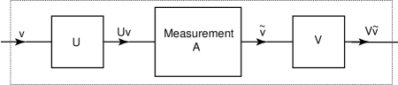
Figure 2: A representation of a measurement of $\mathbf{A}^{\prime}$. A unitary transformation, U, transforms the input state, v, into Uv. Measurement $\mathbf{A}$ is performed on this state, and the output state, $\tilde{\textsf{v}}$, of the measurement is transformed by the unitary transformation V into $\textsf{V}\tilde{\textsf{v}}$.

First, from Postulate 1.1 and the assumption of repetition consistency, there exist $N$ states $\textsf{v}_{1}^{\prime},\textsf{v}_{2}^{\prime},\ldots,\textsf{v}_{N}^{\prime}$ such that measurement $\mathbf{A}^{\prime}$ performed on a system in state $\textsf{v}_{i}^{\prime}$ yields outcome $i$ with certainty. Hence, the arrangement in Fig. 2 must be such that $\mathbf{A}$ yields outcome $i$ with certainty when the input state to the arrangement is $\textsf{v}_{i}^{\prime}$. For this to be the case, U must transform $\textsf{v}_{i}^{\prime}$ to a state of the form $\textsf{v}_{i}e^{i\xi_{i}}$, where $\xi_{i}$ is arbitrary. That is, the matrix U must satisfy the relations

$$\textsf{U}\textsf{v}_{i}^{\prime}=\textsf{v}_{i}e^{i\xi_{i}},\quad i=1,2,\dots,N$$ (85)

Second, if outcome $i$ is obtained from the arrangement, the output state of the arrangement must be of the form $\textsf{v}_{i}^{\prime}e^{i\xi_{i}^{\prime}}$, where $\xi_{i}^{\prime}$ is arbitrary. But, immediately after measurement $\mathbf{A}$, the system is in state $\textsf{v}_{i}$ up to an overall phase. Hence, the matrix V must satisfy the relations

$$\textsf{V}\textsf{v}_{i}=\textsf{v}_{i}^{\prime}e^{i\xi_{i}^{\prime}}\quad i=1,2,\dots,N$$ (86)

From Eq. (84), the $\textsf{v}_{i}$ form an orthonormal basis for $\mathbb{C}^{N}$, and, from Eq. (85), $\textsf{v}_{i}^{\prime}=\textsf{U}^{\dagger}\textsf{v}_{i}e^{i\xi_{i}}$, which, since U is unitary, implies that the $\textsf{v}_{i}^{\prime}$ also form an orthonormal basis. Therefore, any state, v, can be expanded as $\sum_{i}c_{i}^{\prime}\textsf{v}_{i}^{\prime}$, with $c_{i}^{\prime}\in\mathbb{C}$, and the matrices U and V are determined by the relations in Eqs. (85) and (86) up to the $\xi_{i}$ and the $\xi_{i}^{\prime}$.

It is now possible to determine the outcome probabilities if a system in state v undergoes measurement $\mathbf{A}^{\prime}$. Using Eq. (85) and the expansion $\textsf{v}=\sum_{i}c_{i}^{\prime}\textsf{v}_{i}^{\prime}$, the first interaction of the arrangement transforms v into

$$\textsf{U}\left(\sum_{i}c_{i}^{\prime}\textsf{v}_{i}^{\prime}\right)=\sum_{i}c_{i}^{\prime}\textsf{v}_{i}e^{i\xi_{i}}.$$ (87)

The probability that measurement $\mathbf{A}$ in the arrangement yields outcome $i$ is therefore $|c_{i}^{\prime}|^{2}$. Hence, measurement $\mathbf{A}^{\prime}$ performed on the state v yields outcome $i$ with probability $|c_{i}^{\prime}|^{2}$.

In summary, every measurement, $\mathbf{A}^{\prime}\in\mathcal{A}$, has an associated orthonormal basis, $\{\textsf{v}_{1}^{\prime},\textsf{v}_{2}^{\prime},\dots,\textsf{v}_{N}^{\prime}\}$. Such a measurement can be implemented by a measurement $\mathbf{A}$ followed immediately before and after by interactions represented by U and V defined in Eqs. (85) and (86) in terms of these basis vectors. If measurement $\mathbf{A}^{\prime}$ is performed upon a system in state v, the probability, $P_{i}^{\prime}$, of obtaining outcome $i$ is $|c_{i}^{\prime}|^{2}$, where $c_{i}^{\prime}$ is determined by the relation $\textsf{v}=\sum_{i}c_{i}^{\prime}\textsf{v}_{i}^{\prime}$.

Expected Values

If the $i$th outcome of measurement $\mathbf{A}^{\prime}$ has an associated real value $a_{i}^{\prime}$, the expected value obtained in an experiment in which a system in state v undergoes measurement $\mathbf{A}^{\prime}$ is defined as

$$\langle\textsf{A}^{\prime}\rangle=\sum_{i}a_{i}^{\prime}P_{i}^{\prime}.$$ (88)

Since $P_{i}^{\prime}=|c_{i}^{\prime}|^{2}$ and $c_{i}^{\prime}=\textsf{v}_{i}^{\prime{\dagger}}\textsf{v}$, this expression can be also written as

$$\begin{split}\langle\textsf{A}^{\prime}\rangle&=\sum_{i}\textsf{v}^{\dagger}\left(\textsf{v}_{i}^{\prime}a_{i}^{\prime}\textsf{v}_{i}^{\prime{\dagger}}\right)\textsf{v}\\ &=\textsf{v}^{\dagger}\left(\sum_{i}\textsf{v}_{i}^{\prime}a_{i}^{\prime}\textsf{v}_{i}^{\prime{\dagger}}\right)\textsf{v}\\ &=\textsf{v}^{\dagger}\textsf{A}^{\prime}\textsf{v},\end{split}$$ (89)

where the matrix $\textsf{A}^{\prime}\equiv\sum_{i}\textsf{v}_{i}^{\prime}a_{i}^{\prime}\textsf{v}_{i}^{\prime{\dagger}}$ is Hermitian since the $a_{i}^{\prime}$ are real, and is non-degenerate since the $a_{i}^{\prime}$ have been assumed to be distinct (Sec. II.1).

Since the $\textsf{v}_{i}^{\prime}$ are eigenvectors of $\textsf{A}^{\prime}$, with the $a_{i}^{\prime}$ being the corresponding eigenvalues, the matrix $\textsf{A}^{\prime}$ provides a compact mathematical way of representing all the relevant details about measurement $\mathbf{A}^{\prime}$.

IV.4 Composite Systems

It is often the case that a given physical system can be subject to examination in distinct experimental set-ups, where, loosely speaking, the measurements in each set-up probe distinct properties of the system. Formally, we can express this as follows.

Consider a system which admits abstract quantum model, $\mathbf{q}(N^{(1)})$, with respect to measurement set $\mathcal{A}^{(1)}$, and which admits abstract quantum model, $\mathbf{q}(N^{(2)})$, with respect to measurement set $\mathcal{A}^{(2)}$, where the set-ups defined by measurement sets $\mathcal{A}^{(1)}$ and $\mathcal{A}^{(2)}$ are disjoint (in the sense defined in Sec. II). The system can also be modeled as a whole. That is, we can construct the measurement set $\mathcal{A}=\mathcal{A}^{(1)}\times\mathcal{A}^{(2)}$, and construct abstract quantum model $\mathbf{q}(N)$, where $N=N^{(1)}N^{(2)}$. We shall accordingly speak of the system as a composite system consisting of two sub-systems. More generally, if a system admits $d$ ($d>1$) abstract quantum models with respect to $d$ disjoint measurement sets, we shall speak of it as a composite system consisting of $d$ sub-systems.

One often prepares a state of a composite system by first preparing each of its subsystems, and then allowing these subsystems to interact with one another. In order to formally describe such a procedure, one needs a rule, the composite system rule, which we shall now derive, that enables the state of the system to be written down in terms of the states of its sub-systems.

The Composite System Rule

In order to derive the composite system rule, we shall apply Postulate 5 to the case of a composite system with two sub-systems with abstract models $\mathbf{q}(N^{(1)})$ and $\mathbf{q}(N^{(2)})$, respectively, where the composite system has the abstract model $\mathbf{q}(N)$.

Suppose that the sub-systems are in states represented as $(P_{i}^{(1)};\chi_{i}^{(1)})$ and $(P_{j}^{(2)};\chi_{j}^{(2)})$, respectively. Then, by Postulate 5, the state of the composite system can be represented as $(P_{ij};\chi_{ij})$, where

$$P_{ij}=P_{i}^{(1)}P_{j}^{(2)}$$ (90)

$$\chi_{ij}=\chi_{i}^{(1)}+\chi_{j}^{(2)}.$$ (91)

If we write the states of the sub-systems in complex form,

$$\textsf{v}^{(1)}=\left(\sqrt{P_{1}^{(1)}}e^{i\chi_{1}^{(1)}},\sqrt{P_{2}^{(1)}}e^{i\chi_{2}^{(1)}},\dots,\sqrt{P_{N^{(1)}}^{(1)}}e^{i\chi_{N^{(1)}}^{(1)}}\right)^{\text{{T}}}$$

and

$$\textsf{v}^{(2)}=\left(\sqrt{P_{1}^{(2)}}e^{i\chi_{1}^{(2)}},\sqrt{P_{2}^{(2)}}e^{i\chi_{2}^{(2)}},\cdots,\sqrt{P_{N^{(2)}}^{(1)}}e^{i\chi_{N^{(2)}}^{(2)}}\right)^{\text{{T}}},$$

respectively, and, similarly, write the state of the composite system as

$$\textsf{v}=\left(\sqrt{P_{11}}e^{i\chi_{11}},\cdots,\sqrt{P_{N^{(1)},N^{(2)}}}e^{i\chi_{N^{(1)},N^{(2)}}}\right)^{\text{{T}}},$$

then it follows from Eqs. (90) and (91) that v can simply be written as $\textsf{v}^{(1)}\otimes\textsf{v}^{(2)}$.

More generally, consider a composite system with $d$ sub-systems, numbered $1,2,\dots,d$, in states $\textsf{v}^{(1)},\textsf{v}^{(2)},\dots,\textsf{v}^{(d)}$, respectively. We can regard sub-systems $1$ and $2$ as comprising a bipartite composite system, system $1^{\prime}$, which, according to the above result, is in state $\textsf{v}^{(1)}\otimes\textsf{v}^{(2)}$. Next, we can regard system $1^{\prime}$ and sub-system $3$ as comprising a bipartite composite system, system $2^{\prime}$, which is therefore in state $(\textsf{v}^{(1)}\otimes\textsf{v}^{(2)})\otimes\textsf{v}^{(3)}$. Continuing in this way, we can see the state of the composite system with $d$ sub-systems has the state $\textsf{v}=\textsf{v}^{(1)}\otimes\textsf{v}^{(2)}\otimes\dots\otimes\textsf{v}^{(d)}$.

IV.5 Some Generalizations

Representation of sub-system measurements

Suppose that measurement $\mathbf{A}^{(1)}\in\mathcal{A}^{(1)}$, represented by $N^{(1)}$-dimensional Hermitian operator $\textsf{A}^{(1)}$, with eigenstates $\textsf{v}_{i}^{(1)}$ and eigenvalues $a_{i}$, respectively, is performed on sub-system 1 of a bipartite composite system. With respect to the abstract quantum model $\mathbf{q}(N)$ of the composite system, measurement $\mathbf{A}^{(1)}$ is not in the measurement set $\mathcal{A}$ of the composite system since the measurement has only $N^{(1)}$ distinct outcomes whereas a measurement in $\mathcal{A}$ has $N=N^{(1)}N^{(2)}>N^{(1)}$ possible outcomes. However, it is convenient to be able to describe measurement $\mathbf{A}^{(1)}$, which we shall describe as a sub-system measurement, as an $N$-dimensional operator A, in the framework of $\mathbf{q}(N)$.

To determine the form of A, it is sufficient to consider the effect of A on product states of the form $\textsf{v}_{i}^{(1)}\otimes\textsf{v}^{(2)}$ of the composite system, where $\textsf{A}^{(1)}\textsf{v}_{i}^{(1)}=a_{i}\textsf{v}_{i}^{(1)}$. If the composite system is in such a state, then sub-system 1 is in state $\textsf{v}_{i}^{(1)}$. Therefore, when measurement $\mathbf{A}^{(1)}$ is performed, outcome $a_{i}$ is obtained with certainty, and the state of sub-system 1 is unchanged (up to an irrelevant overall phase). Therefore, the state of the composite system remains unchanged. If we require that A has eigenvectors $\textsf{v}_{i}^{(1)}\otimes\textsf{v}^{(2)}$, with respective eigenvalues $a_{i}$, it follows that A can be taken to be $\textsf{A}^{(1)}\otimes\textsf{I}^{(2)}$, where $\textsf{I}^{(2)}$ is the identity matrix in the model of sub-system 2, with the only freedom being a physically irrelevant overall phase in each of the eigenstates of $\textsf{A}^{(1)}$.

The above result trivially generalizes to the case of a measurement performed on one sub-system of a composite system consisting of $d$ sub-systems.

Degenerate measurements

The model $\mathbf{q}(N)$, whose explicit mathematical form has been derived above, applies to an abstract set-up where the measurements, chosen from the set $\mathcal{A}$, have $N$ possible outcomes and therefore, by the distinctness assumption of Sec. II.1, necessarily have $N$ distinct outcome values. From the above discussions, it follows that each measurement $\mathbf{A}\in\mathcal{A}$ is represented by a non-degenerate Hermitian operator of dimension $N$.

Now, it is useful to be able to describe measurements within the context of model $\mathbf{q}(N)$ which have fewer than $N$ outcomes. An example of such measurements that we have discussed above are sub-system measurements. We shall now broaden the discussion to allow for measurements with $N^{\prime}<N$ possible outcomes where $N^{\prime}$ is not a multiple of $N$ and which therefore cannot be regarded as sub-system measurements.

Consider an abstract set-up where a preparation implemented using a measurement from $\mathcal{A}$ is followed by measurement $\mathbf{A}$, whose observable outcome probabilities are denoted $P_{1},\dots,P_{N}$. Suppose that, if measurement $\mathbf{B}$ (with $N^{\prime}<N$) possible outcomes) replaces measurement $\mathbf{A}$, the outcome probabilities, $P_{1}^{\prime},\dots,P_{N^{\prime}}^{\prime}$ of measurement $\mathbf{B}$ can be determined from the $P_{i}$ by a many-to-one map of the outcomes of $\mathbf{A}$ to the outcomes of $\mathbf{B}$. For example, in the case where $N=3$ and $N^{\prime}=2$, the map from the outcomes of $\mathbf{A}$ to the outcomes of $\mathbf{B}$ might consist in $1\rightarrow 1^{\prime}$, $2\rightarrow 2^{\prime}$ and $3\rightarrow 2^{\prime}$, in which case $P_{1}^{\prime}=P_{1}$ and $P_{2}^{\prime}=P_{2}+P_{3}$. In such a case, we shall say that measurement $\mathbf{B}$ is a degenerate form of measurement $\mathbf{A}$; or, more simply, that measurement $\mathbf{B}$ is a degenerate measurement.

Now, measurement $\mathbf{B}$ can formally be treated as if it has $N$ possible outcomes, but where some of these outcomes have the same value. In this mode of description, in the above example, one can maintain a one-to-one map between the outcomes of $\mathbf{A}$ and of $\mathbf{B}$ (so that $1\rightarrow 1^{\prime}$, $2\rightarrow 2^{\prime}$ and so on), but label the outcomes of $\mathbf{B}$ with their outcome values, and, when computing the outcome probabilities of $\mathbf{B}$, group together the outcomes with the same outcome value. In the above example, one would respectively label the three outcomes with outcome values $b_{1},b_{2}$ and $b_{3}$, and but have $b_{2}=b_{3}$.

Since measurement $\mathbf{B}$ is a degenerate form of measurement $\mathbf{A}$, it can be represented by the $N$-dimensional degenerate Hermitian operator $\textsf{B}=\sum_{i}b_{i}\textsf{v}_{i}\textsf{v}_{i}^{\dagger}$, where $\textsf{A}\textsf{v}_{i}=a_{i}\textsf{v}_{i}$. The outcome probabilities for measurement $\mathbf{B}$ can then be computed in the usual way, on the understanding that those outcomes with the same outcome values must not be regarded as physically distinguishable, but must be grouped as just described.

Conversely, in an abstract set-up where $\mathcal{A}$ contains measurements represented by all possible non-degenerate Hermitian operators, a degenerate Hermitian operator can be regarded as representing a measurement which is a degenerate form of some measurement in $\mathcal{A}$.

V Discussion

V.1 General discussion of the Formulation

Above, we have formulated a set of background assumptions (partitioning, time, and states), an abstract experimental set up, and a set of postulates, from which we have shown that it is possible to derive the finite-dimensional abstract quantum formalism (apart from the explicit form of the temporal evolution operator, which will be derived in Paper II).

As described earlier, the background assumptions and the postulates have been formulated as far as possible so that they possess the properties of transparency and traceability. The background assumptions and a number of the postulates (Postulates 3, 3.1, 3.3) are drawn unchanged from the framework of classical physics, and most of the remaining postulates are drawn from the framework of classical physics but modified in light of experimental facts (Postulate 1.1), or are based on a classical-quantum correspondence argument (Postulates 2.1, 2.4, 3.2, 3.4, 5). Hence, the majority of the background assumptions and postulates can be traced to facts or principles that are, or can be, well grounded or reasonably well grounded in experimental facts or in our theoretical intuition.

Of the remaining, novel postulates (Postulates 1.2, 2.2, 2.3, 4), Postulate 1.2 is a direct generalization of experimental facts, and Postulate 4 is a reasonable consistency principle. Postulates 2.2 and 2.3 are both transparent in that they can be clearly understood as assertions about the physical world, and Postulate 2.3 is traceable to a plausible theoretical principle. Furthermore, since Postulates 2.2 and 2.3, in conjunction with the above-mentioned postulates, give rise to the abstract quantum formalism, there is good reason to believe that they are valid. Nevertheless, these two postulates, particularly Postulate 2.2, are less well grounded in our theoretical intuition than the others, and since they play such a key role in the emergence of the quantum formalism, they shall be discussed further below.

We mention briefly that it is also possible to understand some of the postulates using concepts that have not been mentioned thus far. For example, Postulate 2.1 implies that, when a measurement is performed on a system, there are degrees of freedom in the state of a system about which no information is gained. Hence, Postulate 2.1 can be regarded as a concrete expression of Bohr’s principle of complementarity. Consequently, it is possible for different measurements in the measurement set, $\mathcal{A}$, to be inequivalent in that they yield inequivalent information about the state of the system. If one accordingly regards measurements in $\mathcal{A}$ as providing distinct, inequivalent points of view of a physical system, then two questions arise which do not arise in classical physics, namely (a) how should one theoretically represent these different measurements, and (b) whether some measurements yield more information about the state of a system than other measurements. Postulate 1.2 answers the first question by asserting that it is possible to represent all measurements in $\mathcal{A}$ in terms of any given measurement in $\mathcal{A}$ and appropriately chosen interactions in the interaction set, $\mathcal{I}$. Postulate 2.3 answers the second question with the assertion that none of these points of view are privileged insofar as the amount of information they yield about the system, which can be regarded as a kind of principle of relativity applied to the perspectives provided by the different measurements in $\mathcal{A}$.

The derivation itself is noteworthy in several respects. First, it gives rise to a mathematical structure that is neither more nor less general than the finite-dimensional abstract quantum formalism. Therefore, any change to the formalism would require a modification of the postulates or background assumptions. Consequently, as we shall illustrate below, the derivation provides an excellent ‘laboratory’ for investigating proposed modifications of the quantum formalism.

Second, the derivation yields the conclusion that physical transformations are represented either by unitary or antiunitary transformations. This is a rather remarkable, unanticipated feature of the derivation since antiunitary transformations are not generally regarded as an integral part of the abstract quantum formalism (as formalized, for instance, by Dirac or von Neumann), but are instead usually introduced by reference to the theorem of Wigner Wigner-group-theory mentioned in the Introduction. In addition, we note that antiunitary transformations have not been obtained in any of the recent attempts to derive the quantum formalism in which a significant fraction of the quantum formalism is obtained Caticha98b ; Caticha99b ; Hardy01a ; Hardy01b ; Clifton-Bub-Halvorson03 ; Grinbaum03 ; Grinbaum04 . Furthermore, since unitary and antiunitary transformations emerge simultaneously in the above derivation, the derivation suggests that antiunitary transformations are, in fact, an integral part of the quantum formalism.

Third, the derivation shows that the use of complex numbers in the quantum formalism is directly connected with the fact that the set of possible physical transformations can be represented by the set of all unitary or antiunitary transformations of a suitably defined complex vector space. Specifically, the complex form of the quantum state and the (anti)unitarity of physical transformations arise simultaneously as a result of imposing Postulate 3.2 which, in turn, is based on the simple idea that a change in the overall value of the $S_{i}$ in the Hamilton-Jacobi model has no physically observable consequences. Hence, the derivation significantly elucidates the use of complex numbers in the quantum formalism.

Fourth, it is apparent from the derivation that the concept of information plays a substantial role in giving rise to the quantum formalism. The information gain condition directly leads to $Q$-space, which introduces square-roots of probability, or real amplitudes and, via Postulate 2.3, leads to a $2N$-dimensional $Q$-space. Furthermore, in conjunction with Postulate 2.4, Postulate 2.3 leads to the function $f(\chi_{i})=\pm\cos(a\chi_{i}+b)$. Hence, the sinusoidal functions into which the phases in a quantum state enter can be directly traced to the concept of information. Finally, the prior over the unit hypersphere in $Q^{2N}$-space induced by the imposition of Postulate 2.3 leads, via Postulate 4, to the strong constraint that physical transformations can only be represented by orthogonal transformations of the unit hypersphere.

Fifth, the formulation highlights the physical importance of the notion of a prior over a continuous parameter. The notion plays a key role in the derivation, entering through the definition of the Shannon-Jaynes entropy and through Postulate 2.4. This is noteworthy since the notion of prior appears to be underappreciated, occurring rather infrequently in discussions of the probabilistic aspects of quantum theory, and not occurring in most of the aforementioned deductive approaches to quantum theory (the approach due to Caticha Caticha98b ; Caticha99b being the only exception).

Sixth, from the perspective provided by the derivation, one can see rather clearly which assumptions quantum theory shares with classical physics, which assumptions are modifications of classical ideas in light of experimental facts, which assumptions are drawn from classical physics using a correspondence argument, and which are novel insofar as they have no classical counterparts. In particular, one can see that the new ideas that need to be introduced beyond those familiar from classical physics in order to obtain the quantum formalism all arise from the concepts of probability, information, or from classical-quantum correspondence arguments. Since ideas concerning probability and correspondence played an important role in the historical development of quantum theory and in its interpretation in the years immediately following its formulation, the concept of information is the obvious new addition.

Discussion of Postulate 2.2.

Postulate 2.2 introduces the assumption that, when a measurement is performed on a physical system, there are outcomes (which we have labeled $a$ and $b$, and $+$ and $-$) that are objectively realized, but go unobserved by the experimenter.

The apparently successful derivation of the quantum formalism lends support to the plausibility of the assumption that a measurement generates unobserved outcomes. As mentioned above, the assumption also has the benefit of transparency. Nevertheless, it raises two natural questions, namely (i) to what physical property or properties should the outcomes $a$ and $b$, and $+$ and $-$ be attributed, (ii) why are these outcomes not observed in standard experiments. A preliminary response to these questions is as follows.

First, by examining the quantum model of a structureless particle in the classical limit (as $m$ tends to macroscopic values), we have seen that, for a system in an eigenstate of energy, the variable $\chi_{i}$ in the quantum model corresponds to $S_{i}$ in the discretized form of the classical Hamilton-Jacobi model. Now, the $S_{i}$ encode the local momenta and total energy of the system. Hence, if a position measurement is performed and yields the observed outcome $i$, then we can associate the outcomes $a,b$ and $+,-$ with the local momenta and the total energy of the system.

More generally, if a measurement $\mathbf{A}$ is performed on a system, it seems reasonable to associate the outcomes $a,b$ and $+,-$ with the property $A^{\prime}$, which is complementary to property $A$, and with the total energy, $E$, of the system. We shall say that property $A^{\prime}$ is complementary to the property $A$ measured by $\mathbf{A}$ in the sense that exact knowledge of the properties $A$ and $A^{\prime}$ suffice to determine the classical state of the system.

Second, the unobservability of the outcomes $a,b$ and $+,-$ may be roughly understood as follows. We shall see in Paper II that, for a system in an eigenstate of energy $E$, the overall phase, $\chi$, of its quantum state (in the complex representation) changes at the rate $-E/\hbar$. A measurement which is able to resolve the outcomes  $a,b$ and $+,-$ must therefore have a temporal resolution $\Delta t<\hbar/E$. Now, according to the energy-time uncertainty relation $\Delta E\Delta t\geq\hbar/2$ , the energy associated with the interaction used to implement the measurement has uncertainty $\Delta E\geq\frac{1}{2}\hbar/\Delta t$, so that $\Delta E\geq E/2$. From $E=mc^{2}$, it then follows that $\Delta E$ must be of the order of the rest energy of the system. A measurement of such energy would therefore probably not preserve the identity of the system, thereby violating the assumption that interactions preserve the identity of the system (see Sec. II.1). Hence, a measurement with the requisite temporal resolution cannot be consistently described within the quantum formalism. Conversely, a measurement that, with high probability, preserves the identity of the system, will have insufficient temporal resolution to resolve the outcomes $a,b$ and $+,-$.

Discussion of Postulate 2.3

The information gain condition plays a key role in the above derivation via Postulate 2.3. In order to obtain a clearer understanding of the condition, it is helpful to ask whether it resembles, or is equivalent to, other informational principles, or has other consequences which coincide with well-known results. Below, we shall outline two of the consequences which are in agreement with results that are well-known in probability theory and statistics, and shall outline the connections to two other informational principles that have been proposed in the context of recent informational approaches to quantum theory.

First, we have shown elsewhere Goyal05a that the assumption that the information gain condition applies to a probabilistic source is equivalent to Jeffreys’ rule Jeffreys39 , a general rule for the assignment of prior probabilities which was first suggested in the context of probability theory. This rule is widely used in some areas (in econometrics, for example), and yields priors for parameterized probability distributions (such as for the mean and standard deviation of a Gaussian distribution) that are in agreement with the results of other, independent lines of argument (see Jaynes68 , for example).

We also note that the metric $ds^{2}=\sum_{i}dQ_{i}^{2}$, introduced in Sec. IV.1, provides a natural measure of the distance between probability distributions, and is equivalent, up to an irrelevant multiplicative constant, to the Fisher metric, $ds_{F}^{2}=\sum_{i}dP_{i}^{2}/P_{i}$, which measures the distance between the probability distributions $\vec{P}$ and $\vec{P}+\delta\vec{P}$.

Second, we note that the Fisher metric was obtained in Wootters-statistical-distance as a natural measure of the distance between probability distributions, where it was connected with the Hilbert space distance between pure states. The Fisher metric also gives rise to the so-called Fisher information of a continuous probability distribution, which is central to the Fisher information approach to understanding quantum theory Frieden-Schroedinger-derivation ; Reginatto-Schroedinger-derivation .

Finally, we note that, if the information gain condition applies to a probabilistic source with some probability n-tuple, $\vec{P}$, it follows that, in $n$ interrogations of the source, the amount of Shannon-Jaynes information provided by the data about $\vec{P}$ is an increasing function of $n$ in the limit as $n\rightarrow\infty$. This condition, which we shall call the condition of information increase, accords with the rather simple and intuitively plausible idea that, as one gathers more data from a probabilistic source, one’s information about $\vec{P}$ strictly increases. This condition was first proposed, in a slightly different form, in Summhammer99 , where it forms the basis for an attempt to derive a part of the quantum formalism.

Hence, it appears that the information gain condition has a number of interesting and important connections to results in probability theory and to principles in various informational approaches to quantum theory.

V.2 Some Implications of the Deduction

Information in Quantum Theory

One of the major objectives of the programme of deriving quantum theory using the concept of information is to determine whether the concept of information is indispensable to our understanding of the quantum formalism, and, if so, to illuminate the precise relationship between the concept of information and the quantum formalism.

On the first issue, although many recent approaches to derive the quantum formalism involve the concept of information, the conclusion that information is indispensable to our understanding of the quantum formalism cannot be drawn, either because the approaches are unable to obtain the quantum formalism (even though they are able to derive specific results, such as Malus’ law), or because, in those approaches that are able to obtain a significant fraction of the quantum formalism, the abstract nature of some of the assumptions that are employed obscures the role played by information in determining the formalism. Indeed, further doubt on the need for information is cast by other recent approaches, most notably due to Hardy Hardy01a ; Hardy01b , that are successful in deriving a significant fraction of the quantum formalism without invoking the concept of information in any way.

On the second issue, it is remarkable that the manner in which the concept of information is formalized differs considerably amongst the various informational approaches. Consequently, as we shall elaborate upon below, the question of precisely how one should formalize the concept of information in the quantum setting has received a wide range of often incompatible answers. However, it is difficult to evaluate the relative merits of these answers, for the same reasons just given above, namely either because the approaches are too incomplete or because they use abstract assumptions that obscure the role played by information.

The formulation presented here provides significant new insight into both of these issues. First, the formulation rests on assumptions that are transparent and that are, to a large extent, traceable to familiar or well-established experimental facts or theoretical ideas. For example, abstract assumptions that directly introduce complex numbers are avoided. As a result, the role played by information in the derivation can be clearly seen, and its role is sufficiently widespread that it seems very likely that the concept of information could indeed have a fundamental role to play in our understanding of the origin of the quantum formalism.

In order to discuss the second issue, it is convenient to classify the above-mentioned differences in the formalization of the concept of information with respect to (a) what the information is about, (b) whether or not information is quantified in some way, (c) which information measure is chosen, and (d) when the Shannon-Jaynes measure is used, whether there is a naturally preferred prior, and, if so, what is the form of the prior.

In particular, with respect to (a), in Wootters80 , information gain is, as in our approach, regarded as the gain of information about the state of the system due to the receipt of data obtained through performing a measurement on the system. In contrast, in Brukner02b , information gain is taken to be the removal of the uncertainty of the experimenter about the outcome of a measurement as a result of the measurement being performed. In respect to (b), one finds that, for example, in Popescu-Rohrlich97 ; Clifton-Bub-Halvorson03 , information is not subject to quantification, whereas in Brukner02b ; Wootters80 , a particular quantification measure is employed.

With respect to (c), the Shannon-Jaynes entropy is used in Wootters80 , whereas Brukner02b employs a measure that differs from the Shannon entropy, it being argued that the Shannon entropy is inapplicable in the quantum setting Brukner02a . Finally, with respect to (d), some authors Fuchs02 appear to hold the view that there is no natural basis for determining a prior for the Shannon-Jaynes entropy, while, in the field of probability theory, authors who have sought plausible general principles for the assignment of priors have obtained different priors over probability n-tuples (for example, see Jeffreys39 ; Jaynes68 ) on the basis of their arguments.

The approach described here supports the view that information is primarily to be regarded as information gained about the state of a system by an experimenter as a result of performing measurements on the system. In addition, the approach demonstrates the importance of information quantification, and provides significant support for the view that the Shannon-Jaynes entropy is the appropriate information measure in a quantum setting.

Finally, we have shown that, for an experimenter who receives a system prepared in a pure but unknown state, it is possible to formalism an intuitively plausible principle (Postulate 2.3) which determines the prior for the probabilistic source that models a measurement performed on the system by the experimenter. As described in Sec. II.1, one can see that the experimenter’s state of knowledge in this case is not arbitrarily chosen, but precisely reflects the knowledge that a system has been prepared in such a way that its pre-preparation history is irrelevant insofar as the outcomes of subsequent measurements in the set-up are concerned (a preparation which is analogous to an idealized complete preparation in classical physics) and therefore has fundamental physical significance.

Interpretation and Modification of Quantum Theory

The deductive formulation has several implications for some issues of concern in the interpretation of quantum theory, and for some of the proposed modifications of quantum theory. We shall briefly outline one example.

Modification of the Quantum Formalism.

Since the development of the quantum formalism, there has been some uncertainty as to whether the formalism is the most general formalism for the description of quantum phenomena. Various possibilities have been suggested for the generalization of the formalism which, from a purely mathematical point of view, seem to be plausible, and which may have interesting physical consequences. For example, the possibility of non-unitary temporal evolution has been considered by several authors Weinberg89a ; Weinberg89b ; Herbert82 .

In some cases, it is possible to devise experimental tests to rule out certain types of modification on physical grounds. However, it is not always possible to devise such tests or to implement them. The deductive formulation described here provides another way in which the physical plausibility of a proposed modification may be assessed.

The deductive formulation shows that a set of postulates implies the existing quantum formalism. Hence, if any proposed modification of the formalism is to be valid, one or more of these postulates must be changed in some way. By tracing the dependency of the features of the quantum formalism that are at issue to specific postulates, and assessing the consequences of modifying one or more of these postulates, one can potentially use the deductive formulation to obtain another indication as to whether a proposed modification is physically plausible. Furthermore, the formulation has the potential to allow one to explicitly work out the effect that specific changes to particular postulates would have upon the quantum formalism.

For example, for the purpose of illustrating how the deductive formulation can help guide modifications to quantum formalism, suppose that one wishes to modify the quantum formalism so as to allow continuous transformations to be represented by non-unitary transformations. Now, in the deductive formulation, unitarity depends most directly upon Postulate 3.2 (Invariance), and additionally depends upon several supporting postulates which are based on classical physics, on probabilistic ideas, or on novel assumptions. The proposed modification implies that one or more of these postulates needs to be modified.

Amongst the supporting postulates, all but Postulate 2.2 have a reasonably high degree of certainty. However, it does not appear to be possible to modify Postulate 2.2 in any plausible manner so as to give rise to non-unitary transformations. The most likely candidate for modification therefore appears to be Postulates 3.2.

Consider the extreme case where the constraint imposed by Postulate 3.2 is entirely removed. Then, the set of possible transformations consists of the set of orthogonal transformations of the unit hypersphere in $Q^{2N}$. When expressed in complex form, this set of transformations contains transformations that are neither unitary nor antiunitary. Thus, a simple modification of the postulates readily yields a set of non-unitary transformations which can then be subjected to further examination to assess their physical significance and plausibility.

VI Conclusion

In this paper, we have shown that majority of the finite-dimensional abstract quantum formalism can be derived from a set of physically comprehensible assumptions. The derivation illuminates the physical origin of the quantum formalism and the role played by information in quantum theory, makes clearer the commonalities and differences in the assumptions underlying quantum physics and classical physics, and potentially has significant implications for the interpretation and proposed modifications of quantum theory.

Appendix A Implementation of the Information Gain Condition

In this appendix, we shall more formally implement the information gain condition (Sec. IV.1) in the general case of an $M$-outcome probabilistic source.

First, we parameterize the n-tuple $\vec{P}$ by the $(M-1)$–dimensional parameter n-tuple $\underline{\lambda}=(\lambda_{1},\lambda_{2},\dots,\lambda_{M-1})$, so that $\vec{P}=\vec{P}(\underline{\lambda})$, where the parametrization is invertible and differentiable, and then set the prior probability, $\Pr(\underline{\lambda}|\text{I})$, equal to a constant.

Next, we determine $\Pr(\underline{\lambda}|\vec{f},n,\text{I})$. From Bayes’ theorem, the posterior probability is given by

$$\begin{split}\Pr(\underline{\lambda}|\vec{f},n,\text{I})&=\frac{\Pr(\vec{f}|\underline{\lambda},n,I)\Pr(\underline{\lambda}|n,\text{I})}{\idotsint\Pr(\vec{f}|\underline{\lambda},n,I)\Pr(\underline{\lambda}|n,\text{I})\,d\lambda_{1}\dots\,d\lambda_{M-1}}\\ &=\frac{\Pr(\vec{f}|\underline{\lambda},n,\text{I})}{\idotsint\Pr(\vec{f}|\underline{\lambda},n,\text{I})\,d\lambda_{1}\dots\,d\lambda_{M-1}}.\\ \end{split}$$ (92)

Here, we have used the fact that $\Pr(\underline{\lambda}|n,\text{I})=\Pr(\underline{\lambda}|\text{I})$. This follows from an application of Bayes’ theorem, $\Pr(\underline{\lambda}|n,\text{I})\Pr(n|\text{I})=\Pr(n|\underline{\lambda},\text{I})\Pr(\underline{\lambda}|\text{I})$, and the fact that $n$ is chosen freely by the experimenter and therefore cannot depend upon $\underline{\lambda}$. Hence, the posterior probability is proportional to the likelihood, $\Pr(\vec{f}|\underline{\lambda},n,\text{I})$.

When $n$ is large, using Stirling’s approximation, $n!=n^{n}(2\pi n)^{1/2}e^{-n}+\text{O}(1/n)$, the likelihood (Eq. (9)) becomes

$$\begin{split}\Pr(\vec{f}|\underline{\lambda},n,\text{I})&=\frac{(2\pi n)^{1/2}}{(2\pi n)^{M/2}}\frac{1}{\sqrt{f_{1}f_{2}\dots f_{M}}}\prod_{i}\left(\frac{P_{i}(\underline{\lambda})}{f_{i}}\right)^{nf_{i}}\\ &=\frac{(2\pi n)^{1/2}}{(2\pi n)^{M/2}}\frac{1}{\sqrt{f_{1}f_{2}\dots f_{M}}}\\ &\quad\quad\quad\quad\quad\times\exp\left(-n\sum_{i}f_{i}\ln\frac{f_{i}}{P_{i}(\underline{\lambda})}\right).\\ \end{split}$$ (93)

In the limit of large $n$, the posterior, $\Pr(\underline{\lambda}|\vec{f},n,\text{I})$ is sharply peaked about $\underline{\lambda}^{(0)}$, defined by $\vec{f}=\vec{P}(\underline{\lambda}^{(0)})$. To find the form of the posterior about $\underline{\lambda}^{(0)}$, we expand the likelihood about $\underline{\lambda}^{(0)}$. We write

$$P_{i}(\underline{\lambda})=P_{i}(\underline{\lambda}^{(0)})+\sum_{l=1}^{M-1}\frac{\partial P_{i}}{\partial\lambda_{l}}\Bigg{|}_{\underline{\lambda}^{(0)}}(\lambda_{l}-\lambda_{l}^{(0)})+\dots,$$ (94)

and note that

$$\begin{split}\sum_{i}f_{i}\ln\left(\frac{P_{i}(\underline{\lambda})}{f_{i}}\right)&=\sum_{i}f_{i}\ln\left(1+\frac{1}{f_{i}}\sum_{l}\frac{\partial P_{i}}{d\lambda_{l}}(\lambda_{l}-\lambda_{l}^{(0)})+\frac{1}{2f_{i}}\sum_{l,l^{\prime}}\frac{\partial^{2}P_{i}}{d\lambda_{l}d\lambda_{l^{\prime}}}(\lambda_{l}-\lambda_{l}^{(0)})(\lambda_{l^{\prime}}-\lambda_{l^{\prime}}^{(0)})+\dots\right)\\ &=\sum_{i}f_{i}\left(\frac{1}{f_{i}}\sum_{l}\frac{\partial P_{i}}{d\lambda_{l}}(\lambda_{l}-\lambda_{l}^{(0)})+\frac{1}{2f_{i}}\sum_{l,l^{\prime}}\frac{\partial^{2}P_{i}}{d\lambda_{l}d\lambda_{l^{\prime}}}(\lambda_{l}-\lambda_{l}^{(0)})(\lambda_{l^{\prime}}-\lambda_{l^{\prime}}^{(0)})+\dots\right)\\ &-\sum_{i}\frac{f_{i}}{2}\left(\frac{1}{f_{i}}\sum_{l}\frac{\partial P_{i}}{d\lambda_{l}}(\lambda_{l}-\lambda_{l}^{(0)})+\frac{1}{2f_{i}}\sum_{l,l^{\prime}}\frac{\partial^{2}P_{i}}{d\lambda_{l}d\lambda_{l^{\prime}}}(\lambda_{l}-\lambda_{l}^{(0)})(\lambda_{l^{\prime}}-\lambda_{l^{\prime}}^{(0)})+\dots\right)^{2}+\dots\\ &=\left[P_{i}(\underline{\lambda})-P_{i}(\underline{\lambda}^{(0)})\right]\\ &\quad-\frac{1}{2}\sum_{l}\sum_{l^{\prime}}\sum_{i}\frac{1}{f_{i}}\frac{\partial P_{i}}{d\lambda_{l}}\frac{\partial P_{i}}{d\lambda_{l^{\prime}}}(\lambda_{l}-\lambda_{l}^{(0)})(\lambda_{l^{\prime}}-\lambda_{l^{\prime}}^{(0)})+O\left((\lambda_{l}-\lambda_{l}^{(0)})^{3}\right)\\ &=-\frac{1}{2}\sum_{l}\sum_{l^{\prime}}\sum_{i}\frac{1}{f_{i}}\frac{\partial P_{i}}{d\lambda_{l}}\frac{\partial P_{i}}{d\lambda_{l^{\prime}}}(\lambda_{l}-\lambda_{l}^{(0)})(\lambda_{l^{\prime}}-\lambda_{l^{\prime}}^{(0)})+O\left((\lambda_{l}-\lambda_{l}^{(0)})^{3}\right),\end{split}$$ (95)

where the $\ln$ term has been expanded out and we have used the fact that $\sum_{i}P_{i}=1$. Retaining only the leading order terms in the $\lambda_{l}$, the likelihood becomes

$$\begin{split}\Pr(\vec{f}|\underline{\lambda},n,\text{I})&=\frac{(2\pi n)^{1/2}}{(2\pi n)^{M/2}}\frac{1}{\sqrt{f_{1}f_{2}\dots f_{M}}}\\ &\prod_{l=1}^{M-1}\prod_{l^{\prime}=1}^{M-1}\exp\left(-\frac{(\lambda_{l}-\lambda_{l}^{(0)})(\lambda_{l^{\prime}}-\lambda_{l^{\prime}}^{(0)})}{2\sigma_{ll^{\prime}}^{2}}\right),\end{split}$$ (96)

where

$$\frac{1}{\sigma_{ll^{\prime}}^{2}}=n\sum_{i=1}^{M}\frac{1}{P_{i}(\underline{\lambda}^{(0)})}\frac{\partial P_{i}}{\partial\lambda_{l}}\Bigg{|}_{\underline{\lambda}^{(0)}}\frac{\partial P_{i}}{\partial\lambda_{l^{\prime}}}\Bigg{|}_{\underline{\lambda}^{(0)}}.$$ (97)

The posterior can then be obtained from Eq. (92). For example, in the case where $M=2$,

$$\begin{split}\Pr(\lambda_{1}|\vec{f},n,\text{I})&=\frac{\Pr(\vec{f}|\lambda_{1},n,I)}{\int\Pr(\vec{f}|\lambda_{1},n,I)\,d\lambda_{1}}\\ &=\frac{1}{\sigma_{11}\sqrt{2\pi}}\exp\left(-\frac{(\lambda_{1}-\lambda_{1}^{(0)})^{2}}{2\sigma_{11}^{2}}\right),\end{split}$$ (98)

and, more generally,

$$\begin{split}\Pr(\underline{\lambda}|\vec{f},n,\text{I})&=\frac{(\det B)^{1/2}}{(2\pi)^{(M-1)/2}}\\ &\times\prod_{l=1}^{M-1}\prod_{l^{\prime}=1}^{M-1}\exp\left(-\frac{(\lambda_{l}-\lambda_{l}^{(0)})(\lambda_{l^{\prime}}-\lambda_{l^{\prime}}^{(0)})}{2\sigma_{ll^{\prime}}^{2}}\right),\end{split}$$ (99)

where $B_{ll^{\prime}}=1/\sigma_{ll^{\prime}}^{2}$.

Now, consider an $M$-dimensional real Euclidean space, $Q^{M}$, with axes $Q_{1},Q_{2},\dots,Q_{M}$. If we define the vector $\vec{Q}=(Q_{1},Q_{2},\dots,Q_{M})$ such that $Q_{i}=\sqrt{P_{i}}$ ($0\leq Q_{i}\leq 1$), then every $\vec{Q}$ that represents a probability n-tuple lies on the positive orthant, $\mathit{S}^{M-1}_{+}$, of the unit hypersphere, $\mathit{S}^{M-1}$. Eq. (97) can be then rewritten as

$$\begin{split}\frac{1}{\sigma_{ll^{\prime}}^{2}}&=4n\sum_{i=1}^{M}\frac{\partial Q_{i}}{\partial\lambda_{l}}\Bigg{|}_{\underline{\lambda}^{(0)}}\frac{\partial Q_{i}}{\partial\lambda_{l^{\prime}}}\Bigg{|}_{\underline{\lambda}^{(0)}}.\\ \end{split}$$ (100)

For example, in the case where $M=2$,

$$\begin{split}\frac{1}{\sigma_{11}^{2}}&=4n\left[{\left(\frac{dQ_{1}}{d\lambda_{1}}\right)}^{2}\Bigg{|}_{\lambda_{1}^{(0)}}+{\left(\frac{dQ_{2}}{d\lambda_{1}}\right)}^{2}\Bigg{|}_{\lambda_{1}^{(0)}}\right]\\ &=4n{\left(\frac{ds}{d\lambda_{1}}\right)}^{2}\Bigg{|}_{\lambda_{1}^{(0)}},\\ \end{split}$$ (101)

where $ds^{2}=dQ_{1}^{2}+dQ_{2}^{2}$ is the metric in $Q^{2}$. The posterior, $\Pr(\lambda_{1}|\vec{f},n,I)$, is therefore a Gaussian with standard deviation,

$$\sigma=\frac{1}{2\sqrt{n}}{\left(\frac{ds}{d\lambda_{1}}\right)}^{-1}\Bigg{|}_{\lambda_{1}^{(0)}},$$ (102)

where $s$ is the distance along the positive quadrant of the unit circle. Since $\Pr(\lambda_{1}|\text{I})$ is constant,

$$\begin{split}\Delta K&=\frac{1}{2}\ln\left(\frac{2n}{\pi e}\right)+\ln{\left|\frac{ds}{d\lambda_{1}}\right|}\Bigg{|}_{\lambda_{1}^{(0)}}-\ln\left[\Pr(\lambda_{1}|\text{I})\right]\\ &=\frac{1}{2}\ln\left(\frac{2n}{\pi e}\right)-\ln\left[\Pr\right(s(\lambda_{1}^{(0)})|\text{I}\left)\right]\end{split}$$ (103)

where the relation $\Pr(\lambda_{1}|\text{I})|d\lambda_{1}|=\Pr(s|\text{I})|ds|$ has been used to arrive at the second line. Independence of $\Delta K$ from $f_{1}$ can be ensured if and only if $\Pr(s|\text{I})$ at $\lambda_{1}^{(0)}$ is a constant on $\mathit{S}^{M-1}_{+}$, where the constant is non-zero in order to ensure that the parametrization of $\vec{P}$ is invertible. In this case,

$$\Delta K=\frac{1}{2}\ln\left(\frac{2n}{\pi e}\right)+\text{const.}$$ (104)

Since we assumed at the outset that $\Pr(\lambda_{1}|\text{I})$ is a constant on $\mathit{S}^{M-1}_{+}$, it follows from the relation

$$\Pr(\lambda_{1}|\text{I})|d\lambda_{1}|=\Pr(s|\text{I})|ds|$$ (105)

that $s(\lambda_{1})=a\lambda_{1}+b$, where $a,b$ are arbitrary real constants. From Eq. (102), it then follows that $\sigma=1/2a\sqrt{n}$, and, from Eq. (105), it then follows that the posterior over the positive quadrant of the unit circle is a Gaussian whose standard deviation is $1/2\sqrt{n}$, which is independent of $\vec{Q}$.

The treatment for general $M$ runs parallel to the above. Suppose that the $\lambda_{l}$ are chosen such that infinitesimal changes in the $\lambda_{l}$ generate orthogonal displacements in $Q^{N}$–space. This can be done by using hyperspherical co-ordinates, $(r,\theta_{1},\theta_{2},\dots,\theta_{M-1})$, with $r=1$ and, for $l=1,\dots,M-1$, with $\theta_{l}$ being a function of $\lambda_{l}$ only. In that case, one finds that

$$\sigma_{ll^{\prime}}=\frac{1}{2\sqrt{n}}{\left(\frac{\partial s}{\partial\lambda_{l}}\right)^{-1}}\bigg{|}_{\underline{\lambda}^{(0)}}\,\,\delta_{l,l^{\prime}}.$$ (106)

Consequently, the posterior probability (Eq. (99)) reduces to a product of Gaussian functions,

$$\Pr(\underline{\lambda}|\vec{f},n,\text{I})=\prod_{l=1}^{M-1}\frac{1}{\sigma_{ll}\sqrt{2\pi}}\exp\left(-\frac{(\lambda_{l}-\lambda_{l}^{(0)})^{2}}{2\sigma_{ll}^{2}}\right),$$ (107)

and the information gain becomes

$$\begin{split}\Delta K&=-\sum_{l=1}^{M-1}\ln\bigl{(}\sigma_{ll}\sqrt{2\pi e}\bigr{)}\\ &=\frac{N-1}{2}\ln\left(\frac{2n}{\pi e}\right)+\sum_{l=1}^{M-1}\ln\frac{\partial s}{\partial\lambda_{l}}\Bigg{|}_{\underline{\lambda}^{(0)}}\\ &\quad\quad\quad\quad-\ln\left[\Pr(\lambda_{1},\lambda_{2},\dots,\lambda_{M-1}|\text{I})\right]\\ &=\frac{M-1}{2}\ln\left(\frac{2n}{\pi e}\right)-\ln\left[\Pr(s_{1},s_{2},\dots,s_{M-1}|\text{I})\right],\end{split}$$ (108)

where $ds^{2}=dQ_{1}^{2}+dQ_{2}^{2}+\dots+dQ_{M}^{2}$ and where $ds_{l}=(\partial s/\partial\lambda_{l})|_{\underline{\lambda}^{(0)}}d\lambda_{l}$.

Since the $\lambda_{l}$ are independent variables, independence of $\Delta K$ from the $\lambda_{l}$ can be ensured if and only if the prior $\Pr(s_{1},s_{2},\dots,s_{M-1}|\text{I})$ is a constant on $\mathit{S}^{M-1}_{+}$ independent of the $\lambda_{l}$, in which case

$$\Delta K=\frac{M-1}{2}\ln\left(\frac{2n}{\pi e}\right)+\text{const.}$$ (109)

Therefore, any area element, $dA=\prod_{l=1}^{M-1}d\,s_{l}$, on $\mathit{S}^{M-1}_{+}$ is weighted proportionally to its area independent of its location on the unit hypersphere. Hence, the information gain condition is equivalent to the condition that the prior over $\mathit{S}^{M-1}_{+}$ is uniform.

From the constancy of $\Pr(s_{1},s_{2},\dots,s_{M-1}|\text{I})$ derived above, it follows that $\Pr(s_{1}|\text{I}),\Pr(s_{2}|\text{I}),\dots,\Pr(s_{M-1}|\text{I})$ are all constant. Similarly, from the constancy of $\Pr(\lambda_{1},\lambda_{2},\dots,\lambda_{M-1}|\text{I})$, which we assumed at the outset, follows the constancy of the $\Pr(\lambda_{l}|\text{I})$. From the relations $\Pr(\lambda_{l}|\text{I})d\lambda_{l}=\Pr(s_{l}|\text{I})ds_{l}$ ($l=1,2,\dots,M-1$), it then follows that

$$s_{l}=a_{l}\lambda_{l}+b_{l},$$ (110)

where the $a_{l}$ and $b_{l}$ are arbitrary constants. From Eq. (106), we obtain that

$$\sigma_{ll^{\prime}}=\frac{1}{2a_{l}\sqrt{n}}\,\,\delta_{l,l^{\prime}},$$ (111)

which, using Eq. (110), implies that the posterior over $\mathit{S}^{M-1}_{+}$ is a symmetric Gaussian function whose standard deviation is $1/2\sqrt{n}$, independent of $\vec{Q}$.

References

- (1) C. Rovelli. Relational quantum mechanics. Int. J. Theor. Phys., 35:1637–1678, 1996. See quant-ph/9609002v2.
- (2) S. Popescu and D. Rohrlich. Causality and nonlocality as axioms for quantum mechanics. 1997. See quant-ph/9709026v2.
- (3) C. A. Fuchs. Quantum mechanics as quantum information. May 2002. See quant-ph/0205039.
- (4) J. A. Wheeler. It from bit. In Proceedings of the 3rd international symposium on the foundations of quantum mechanics, Tokyo, 1989.
- (5) J. Summhammer. Maximum predictive power and the superposition principle. 1999. See quant-ph/9910039.
- (6) A. Zeilinger. Found. Phys., 29:631, 1999.
- (7) W. K. Wootters. The acquisition of information from quantum measurements. PhD thesis, University of Texas at Austin, 1980.
- (8) Č. Brukner and A. Zeilinger. Operationally invariant information in quantum measurements. Phys. Rev. Lett., 83:3354–3357, 1999.
- (9) Č. Brukner and A. Zeilinger. Conceptual inadequacy of the Shannon information in quantum mechanics. Phys. Rev. A, 63(022113), 2001.
- (10) Č. Brukner and A. Zeilinger. Information and fundamental elements of the structure of quantum theory. 2002. See quant-ph/0212084v1.
- (11) A. Caticha. Consistency, amplitudes and probabilities in quantum theory. Phys. Rev. A, 57:1572, 1998.
- (12) A. Caticha. Insufficient reason and entropy in quantum theory. 1999. See quant-ph/9810074v2.
- (13) R. Clifton, J. Bub, and H. Halvorson. Characterising quantum theory in terms of information-theoretic constraints. 2003. See quant-ph/0211089v2.
- (14) A. Grinbaum. Elements of information-theoretic derivation of the formalism of quantum theory. Int. J. Quant. Inf., 1(3):289–300, 2003. See also quant-ph/0306079.
- (15) A. Grinbaum. The Significance of Information in Quantum Theory. PhD thesis, Ecole Polytechnique, Paris, 2004. See quant-ph/0410071.
- (16) R. P. Feynman. Space-time approach to non-relativistic quantum mechanics. Rev. Mod. Phys., 20, 1948.
- (17) P. Goyal. An information-theoretic approach to quantum theory, II: The formal rules of quantum theory. 2007.
- (18) E. Wigner. Group Theory. 1959.
- (19) A. Rényi. On the foundations of information theory. Rev. Int. Stat. Inst., 33(1), 1965.
- (20) C. Tsallis. J. Stat. Phys., 52:479, 1988.
- (21) C. E. Shannon. The mathematical theory of communication. Bell Sys. Tech. J., 27:379–423, 1948.
- (22) A. I. Khinchen. The entropy concept in probability theory. In Mathematical foundations of information theory. Dover publications, 1957.
- (23) D. Faddeev. In H. Grell, editor, Arbeiten zum Informationstheorie I, pages 88–91. Deutscher Verlag der Wissenschaften, 1957.
- (24) E. T. Jaynes. Information theory and statistical mechanics I. Phys. Rev., 106:620–630, 1957. Reprinted in Jaynes83 .
- (25) E. T. Jaynes. Information theory and statistical mechanics II. Phys. Rev., 108:171–190, 1957. Reprinted in Jaynes83 .
- (26) E.T. Jaynes. Brandeis lectures. 1963. See section 4b. Reprinted in Jaynes83 .
- (27) L. Hardy. Quantum theory from five reasonable axioms. 2001. See quant-ph/0101012.
- (28) L. Hardy. Why quantum theory? 2001. See quant-ph/0111068v1.
- (29) P. Goyal. Prior probabilities: An information-theoretic approach. In K. Knuth et al., editors, Bayesian Inference and Maximum Entropy Methods, 2005.
- (30) H. Jeffreys. Theory of Probability. Oxford University Press, 1939.
- (31) E.T. Jaynes. Prior probabilities. IEEE Trans. Sys. Sci Cyb., SSC-4:227–241, September 1968. Reprinted in Jaynes83 .
- (32) W. K. Wootters. Statistical distance and Hilbert space. Phys. Rev. D, 23(2), 1981.
- (33) B. R. Frieden and Soffer. Lagrangians of physics and the game of Fisher-information transfer. Phys. Rev. E, 52:2274–2286, 1995.
- (34) M. Reginatto. Derivations of the equations of nonrelativistic mechanics using the principle of minimum Fisher information. Phys. Rev. A, 58:1775–8, 1998.
- (35) S. Weinberg. Phys. Rev. Lett., 62:485, 1989.
- (36) S. Weinberg. Ann. Phys. (N.Y.), 194:336, 1989.
- (37) N. Herbert. Found. Phys., 12:1171, 1982.
- (38) R. D. Rosenkrantz, editor. E.T. Jaynes: Papers on Probability, Statistics, and Statistical Physics. Kluwer, 1983.
- (39) D. S. Sivia. Data Analysis: A Bayesian Tutorial. Oxford Science Publications, 1996.
- (40) E.T. Jaynes. Probability Theory: The logic of science. Cambridge University Press, 2003.
- (41) A. Peres. Quantum Theory: Concepts and Methods. Kluwer, 1995.
- (42) Oppenheim J. Quantum Time. PhD thesis, University of Toronto, 1999.