Fundamentals of universality in one-way quantum computation

Abstract

In this article, we build a framework allowing for a systematic investigation of the fundamental issue: “Which quantum states serve as universal resources for measurement-based (one-way) quantum computation?” We start our study by re-examining what is exactly meant by “universality” in quantum computation, and what the implications are for universal one-way quantum computation. Given the framework of a measurement-based quantum computer, where quantum information is processed by local operations only, we find that the most general universal one-way quantum computer is one which is capable of accepting arbitrary classical inputs and producing arbitrary quantum outputs—we refer to this property as CQ-universality. We then show that a systematic study of CQ-universality in one-way quantum computation is possible by identifying entanglement features that are required to be present in every universal resource. In particular, we find that a large class of entanglement measures must reach its supremum on every universal resource. These insights are used to identify several families of states as being not universal, such as 1D cluster states, GHZ states, W states, and ground states of non-critical 1D spin systems. Our criteria are strengthened by considering the efficiency of a quantum computation, and we find that entanglement measures must obey a certain scaling law with the system size for all efficient universal resources. This again leads to examples of non-universal resources, such as, e.g., ground states of critical 1D spin systems. On the other hand, we provide several examples of efficient universal resources, namely graph states corresponding to hexagonal, triangular and Kagome lattices. Finally, we consider the more general notion of encoded CQ-universality, where quantum outputs are allowed to be produced in an encoded form. Again we provide entanglement-based criteria for encoded universality. Moreover, we present a general procedure to construct encoded universal resources.

1 Introduction

1.1 Role of MQC in fundamental investigations

Quantum computers offer a promising new way of information processing, in which the distinguished features of quantum mechanics can fruitfully be exploited. The discovery of quantum algorithms, most notably Shor’s factoring algorithm [1] and Grover’s search algorithm [2], demonstrate that quantum computation can achieve a (possibly exponential) speed-up over classical devices. This has put quantum computation at the focus of contemporary research, and, indeed, significant progress in the theoretical understanding of quantum information processing, as well as promising steps toward an experimental realization of large-scale quantum computation, have recently been reported. In spite of these exciting developments, the basic question: ’Which features of quantum mechanics are responsible for the speed-up of quantum computation over classical devices?’ remains to date largely unanswered.

An indication that there might not be a straightforward answer to this fundamental but difficult question, is given by the fact that there exist various models for quantum computation, such the quantum Turing machine [3], the quantum circuit (or network) model [4], measurement-based models [5, 6, 7, 8, 9, 10, 11, 12], as well as adiabatic quantum computation [13]. Although these models have been shown to be equivalent in a certain complexity-theoretic sense (colloquially speaking, any problem which can be solved efficiently in one of the above models, can also be solved efficiently by the others), the elementary concepts underlying these schemes may differ significantly.

Therefore, certain computational schemes may lend themselves more than others to understand fundamental issues regarding the power of quantum as compared to classical computation. The new paradigm of measurement-based quantum computation (MQC), with the one-way quantum computer [5, 6] and the teleportation-based model [7, 8] as the most prominent examples, has lead to fresh perspectives in these respects. While in, e.g., the circuit model quantum information is processed by coherent unitary evolutions, in MQC the processing of quantum information takes place by performing sequences of adaptive measurements. Teleportation-based models use joint (i.e., entangling) measurements on two or more qubits and thereby perform sequences of teleportation-based gates. In contrast, the one-way model uses a highly entangled state, the cluster state [14], as a universal resource which is processed by single-qubit measurements only.

The latter property provides the model of one-way quantum computation—which is the focus of this article—with a very distinct feature, namely that the entire resource of the computation is provided by the entangled state in which the system is initialized. In particular, any computational speed-up of such a model w.r.t. classical computation can be traced back entirely to the properties of the resource state.

What is more, in the one-way model the resource character of entanglement is particularly highlighted, as it is clearly separated from the processing of quantum information by local, single-qubit measurements. As the latter cannot increase any entanglement in the system, all entanglement required for quantum computation needs to be initially present in the system. The introductory question of this article can therefore be rephrased in a more concise form, namely ’What are the essential entanglement features of a resource state for (one-way) MQC that are required to obtain a speed-up over classical computation?’ The present article will be centered around this question.

We emphasize that, in the following, we will exclusively consider MQC in the sense of the one-way quantum computer, i.e., considering only local measurements; teleportation-based models will not be considered.

For proposed implementations of measurement-based computation see e.g. Refs. [6, 15, 16, 17, 18, 19, 20, 21, 22] (further references can be found in Ref. [23]); for recent experimental developments see Refs. [24].

1.2 Universality in MQC—aim and contribution of this paper

In this paper, we will be interested in those resource states for MQC which possess the strongest computational power possible, namely those which enable universal quantum computation, as do the 2D cluster states . It is our aim to gain insight under which conditions resource states, other than the 2D cluster states, are universal, and what the role of entanglement plays in this issue.

In order to study universality in MQC in detail, it is necessary to have a clearcut definition of this notion. We will hence start our study (Sec. 2) by re-examining what is exactly meant by “universal quantum computation”, and what the implications are for universality in MQC (Sec. 3). We will find that the notion of universality strongly depends on whether the in- and outputs of a quantum computer are allowed to be either classical or quantum. Furthermore, we will argue that the most general universal one-way quantum computer is a device which accepts arbitrary classical (C) inputs and produces arbitrary quantum (Q) outputs—we will call such a device a CQ-universal one-way quantum computer. The property that a one-way quantum computer is restricted to accept classical information only, is essentially due to the fact that, after the resource state of the device has been prepared, the only allowed quantum operations are local operations, which do not allow one to couple in quantum input states. One the other hand, the generation of arbitrary quantum output states poses no problem (as is the case in the 2D cluster state model)—hence the notion of CQ-universality in MQC. As a standard example, the 2D cluster state model is CQ-universal.

After giving a formal definition of what constitutes a (CQ-)universal resource state for MQC, we develop a framework which allows a systematic investigation of the criteria which need to be met by every universal resource (Sec. 5). Our approach, which has been initiated in Ref. [27], is centered around considerations regarding entanglement. In particular, we find that every universal resource needs to be maximally entangled, in the sense that every entanglement measure (belonging to a well-defined class) must reach its supremum on every universal resource. This result subsequently leads to several criteria for universality, by applying the result to specific measures. We consider several examples and show that entropic entanglement width [27], Schmidt rank width [26], Schmidt measure [28], geometric measure of entanglement [29, 30] as well as measures describing the capability to generate Bell pairs, must grow unboundedly on every universal resource—thus, every resource which does not exhibit a divergence of the above measures, cannot be universal. This leads to several examples of states which are not universal, such as large families of graph states, the GHZ states, W states and ground states of non-critical strongly interacting 1D systems.

Along the way, we also take efficiency into account (Sec. 6). In this case, we find that a necessary condition for efficient universality is that the growth of above mentioned entanglement measures must be sufficiently fast with the system size—in most cases faster-than-logarithmic. These results are again used to provide further examples of states which are not efficiently universal. Furthermore, we also construct examples of efficient universal resource states, namely graph states corresponding to 2D hexagonal, triangular and Kagome lattices (Sec. 7). Here our proof consists of showing explicitly that all these resources can be transformed into each other (with a certain moderate overhead) by local operations and classical communication (LOCC)—and are therefore equally maximally entangled.

In Sec. 8, we consider a weaker (i.e., more general) form of CQ-universality, namely encoded universality, where it is sufficient that the desired output states be generated in an encoded form (here the notion of “encoding” is similar to e.g. schemes in fault-tolerance and quantum error-correction). After discussing encodings and providing a definition for encoded universality, we investigate to which extent entanglement-based criteria can be used to assess encoded non-universality. Most importantly, we show that the Schmidt measure and geometric measure, as well as all measures which are non-increasing under coarsening of partitions of the system, give rise to criteria for encoded universality. Furthermore, relying on an “indirect” argument of classical simulatability of quantum computation, we also argue that the Schmidt rank width provides a criterion for encoded universality. We then also give general constructive results; most importantly, extending results put forward in Ref. [12], we find that any universal resource which is itself subsequently encoded in an arbitrary way, is an encoded universal resource—which is a nontrivial statement. This implies in particular that for any kind of encoding, an encoded 2D-cluster state is an encoded universal resource (up to logical Pauli operations). We provide extensions to encoded universality and discuss some examples of encoded universal resources presented in the literature.

Finally, a summary of our results and an outlook toward further investigations are formulated in Sec. 9 and 10.

Remark 1.

The main text is supplemented with a number of remarks. Although these remarks provide information which is relevant to obtain a detailed understanding of the current investigation, they may be skipped in a first reading. $\diamond$

2 General considerations on universality

In this section, we discuss what a universal quantum computer should be capable of. Somewhat unexpectedly, this is not so trivial as one might think at first sight. In particular, we will argue that there are several possible definitions, all of which are of natural interest depending on which application one might have in mind.

We will start our discussion by reviewing, in section 2.1, some important conceptual notions regarding the universality of the circuit model. In investigations of universality for general computational models, the circuit model will serve as a natural reference. This then leads us, in section 2.2, to consider four natural but distinct notions of universality of a quantum computer, namely CC-, CQ-, QC, and QQ-universality. In each of those notions of universality it is specified whether the computer should accept quantum (Q) or classical (C) inputs, and produce quantum or classical outputs.

2.1 Circuit model

In the circuit model for quantum computation, quantum information is processed by applying sequences of unitary gates on quantum states. These gates are typically chosen from an elementary set. Universality in the circuit model is defined with respect to the possibility of generating arbitrary unitary operations by composition of such elementary gates. Namely, a gate set ${\cal S}$ is called universal if any $n$-qubit unitary operation $U\in SU(2^{n})$, for every $n$, can be realized as a sequence of elementary gates taken from ${\cal S}$.

Notice that in principle the number of gates required to produce a given unitary may be unbounded. In practice, however, the number of gates that can be applied is limited, and one often considers only $n$-qubit unitary operations $U$ that can be generated efficiently, i.e., with poly$(n)$ elementary gates. An example of a universal gate set ${\cal S}_{1}$ is given by the two-qubit CNOT gate together with the group $SU(2)$ of arbitrary single-qubit gates [31], and this specific gate set usually serves as a reference set to distinguish between efficient and non-efficient gate sets. In particular, one says that a set of gates ${\cal S}$ is efficiently universal if any $U\in SU(2^{n})$ that can be efficiently generated—i.e., with poly($n$) gates—using the gate set ${\cal S}_{1}$, can also be efficiently generated using the gate set ${\cal S}$. This implies that efficient universal gate sets can simulate the set ${\cal S}_{1}$ with polynomial overhead.

For many practical applications, the exact generation of a unitary operator is not required, and an approximate application of $U$ with a certain accuracy $\epsilon$ is sufficient. Such a finite accuracy shows up very naturally when considering discrete sets of elementary gates, such as the CNOT gate plus a finite set of single-qubit gates with certain rotational angles [31]. In fact, it turns out that an approximate generation of all unitary operations with arbitrary accuracy is possible for many discrete sets of elementary gates. The best known examples is the set consisting of single- and two-qubit Clifford gates [32] together with a single-qubit $\pi/8$ rotation along the $z$-axis [31]. As established in the Solovay-Kitaev theorem, the overhead to approximate a sequence of $m$ elementary gates from the set ${\cal S}_{1}$ with accuracy $\epsilon$ by gates from the discrete gate set specified above, scales as $O(m\log^{c}(m/\epsilon))$, i.e., poly-logarithmically in $1/\epsilon$ (where $1\leq c\leq 2$) [31, 33].

It is evident from above discussion that universality in the circuit model is concerned with the possibility of implementing arbitrary unitary operations. However, regarding the nature of a quantum computation in the circuit model, often additional (implicit) assumptions are made concerning both the input and output of a computation. Namely, it is often assumed that both the input and the output of a quantum computation are classical. This manifests itself in the fact that, first, the input state of a computation is typically a standard quantum state $|0\rangle^{\otimes n}$ and, second, the last step of the computation—after the unitary operation has been implemented—typically consists of a sequence of single–qubit measurements in the standard basis, destroying the final quantum state (i.e., transforming it to a simple product state) and yielding the classical output. We emphasize that it is not necessary to restrict a quantum computation in the circuit model to this classical input–output scenario. In particular, arbitrary quantum inputs in the form of $n$-qubit quantum states $|\psi\rangle$ can naturally be processed by a (universal) circuit model quantum computer. In addition, it is not necessary to perform a final measurement. Without such final measurements, the quantum computation produces a quantum state as output, which might be used for other purposes. In this general scenario, a circuit model quantum computer might be considered as a device which accepts a quantum state as an input, processes it by applying a unitary operation (representing the program and possible classical input data), and finally produces an output quantum state (together with classical information resulting from possible measurements).

Thus, a (universal) circuit model quantum computer can be regarded as a device which accepts either a classical or quantum input, and which produces either a classical or quantum output. As we will discuss in more detail in section 2.2, the different choices one can make regarding the types of in- and outputs of a quantum computation have a significant impact on the definition(s) of universality one may consider. This will be a crucial point in defining and studying universality in measurement-based quantum computation.

2.2 Different types of universality

As we have briefly reviewed in the previous section, universality in the circuit model is concerned with the possibility of implementing arbitrary unitary operations—be it exactly or with a certain precision.

When considering a quantum computational model other than the circuit model—such as the measurement-based model considered here—one can ask in which sense it may be called universal. In order to define universality, one typically takes the circuit model as a reference, and this is also the strategy which will be adopted here . Colloquially speaking, a model is called universal if it can perform the same tasks as a circuit model quantum computer. In this section, we make this statement more precise (although we will stay at a qualitative level). In particular, we will argue that possible definitions of what a universal quantum computer is supposed to be capable of, depend on the allowed input and output, which may either be of classical or quantum nature.

Regarding in- and outputs of a quantum computation, we have the following possibilities:

• Both input and output are classical;

• The input is quantum and the output is classical;

• The input is classical and the output is a quantum;

• Both input and output are quantum.

The notion of “universal quantum computation” has different meanings depending on which of the above cases is considered. In each of these situations, a natural definition of universality can be formulated where the circuit model is used as a reference. Moreover, we emphasize that we will make a clear separation between universality of a quantum computer and the efficiency with which computations can be executed—i.e., we will regard universality and efficient universality as distinct notions (this point will be discussed further in section 2.3).

We now consider the cases CC, CQ, QC and QQ one by one.

CC.— Here it is assumed that both input and output of the computation are classical, i.e., a quantum computer is considered to be a device that solves classical problems and provides the solution in the form of classical data. Only at an intermediate stage the additional power of quantum mechanics is used to achieve an enhanced processing of information. The final step of such a quantum computation is usually given by a sequence of (local) measurements performed on the output state, which ensures the transition from quantum information to classical information. An important example of this kind is given by Shor’s factoring algorithm. One may call a quantum computer CC-universal if it can perform the same tasks as a circuit model quantum computer which accepts classical inputs and produces classical outputs. That is, for every unitary $U$, a CC-universal quantum computer must be capable of reproducing the statistics of local measurements performed on the state $U|0\rangle^{\otimes n}$. Note that, as we do not take efficiency into account yet, a CC-universal quantum computer is simply one which can perform universal classical computation (and is therefore not different from a classical computer). In order to distinguish a CC-universal quantum computer from classical computers, one needs to take efficiency into account and demand that the classical data is obtained in polynomial time for any unitary operations $U$ that can be generated with a polynomial sized quantum circuit. We refer to remark 2 for further details regarding this issue.

QC.— In this case, the output is still classical, i.e., the final step of the computation is given by a sequence of measurements. However, now the input can be an arbitrary quantum state $|\phi_{\rm in}\rangle$ that is processed by the quantum computer. The input state may be the output state of a previous QQ-quantum computer (see the case QQ below), or the state of some physical system which one would like to study with the help of a (QC) quantum computer, e.g., the ground state of some spin system. For instance, one may wish to learn the value of some observable or entanglement measure, or the fact whether a state (or density operator) has positive partial transposition [34]. Note that the input state may be known or unknown to the device. Finally, also in studies of quantum complexity classes such as QMA, situations are considered where devices can accept quantum states as inputs (”certificates”) [35].

A quantum computer is then called QC-universal if it can perform the same tasks as a circuit model quantum computer which accepts quantum inputs and produces classical outputs. That is, for every (possibly unknown) input state $|\phi_{\rm in}\rangle$ and for every unitary operation $U$, a QC-universal quantum computer can reproduce the statistics of local measurements performed on the quantum state $|\phi_{\rm out}\rangle=U|\phi_{\rm in}\rangle$. One may in addition take efficiency into account, in the same way as in the case of CC, demanding that the overhead with respect to the circuit model is polynomial .

CQ.— Here the input is classical but the output of a quantum computation can now be a quantum state. Compared to a CC quantum computer, this device has the advantage that one can decide at a later stage whether one wishes to obtain classical information by performing measurements, or whether one wants to use the produced state as the input of a following quantum computation, or whether one wants to use this state for another quantum information task—the goal of a quantum computation might e.g. be to produce a quantum state which is subsequently distributed over several parties, and then used to establish a secret key, for secret sharing, or to perform (non-local) two-qubit gates.

Analogous to the previous cases, we will call a quantum computer CQ-universal if it can perform the same tasks as a circuit model quantum computer which accepts classical inputs and which produces quantum outputs. That is, for every unitary operation $U$, a CQ-universal quantum computer is able to produce the quantum state $|\phi_{\rm out}\rangle=U|0\rangle^{\otimes n}$. This definition is equivalent to stating that that a CQ-universal quantum computer is capable of preparing an arbitrary quantum state. One may again add the requirement of efficiency here, calling a quantum computer efficiently CQ-universal if the overhead in the above state preparation compared to the circuit model is polynomial.

QQ.— This is the most powerful device, as it can accept quantum states as input and can produce quantum states as output. Apart from the applications mentioned in (ii) and (iii), such a quantum computer is composable, i.e., the output of a previous quantum computation can be used as the input of a subsequent quantum computation. In particular this allows one to use distributed quantum processors. We will call a quantum computer QQ-universal if it can produce the quantum state $|\phi_{\rm out}\rangle=U|\phi_{\rm in}\rangle$ for any given input state $|\phi_{\rm in}\rangle$ and for any unitary operation $U$. Equivalently, one can say that any unitary operation $U$ can be performed on an arbitrary input state. As before, the notion of efficiency can naturally be considered.

2.3 Some remarks

In this section, we give a number of remarks regarding the above types of universality.

Remark 2.

Separating universality and efficiency.— In the definitions of CC-, CQ-, QC- and QQ-universality we have deliberately separated the issue of universality from the issue of efficiency. The reason for this is that, in the present study of MQC, we will be interested in computational models having a quantum output. In such situations, we will argue that a lot can be learned by studying, say, CQ-universality, without considering efficiency. This will be in particular the case for the study of necessary conditions for CQ-universality: we will present systematic procedures for identifying large classes of resource states for MQC which are not CQ-universal, even though no considerations of efficiency are included. Finally, we note that in the case of CC-universality it is meaningless to separate universality from efficiency; as pointed out above, every classical computer is (inefficiently) CC-universal, such that nothing can be learned about the differences between classical and quantum computation by considering CC-universality without efficiency. $\diamond$

Remark 3.

Qubits, qudits and encodings.— In the above definitions of the different types of universalities, and in the discussion of the circuit model, we have always assumed that the physical systems involved are qubit systems (and qubit systems only). This does not represent a restriction if one considers classical inputs and outputs, as only the information is important in this case; the type and dimension of systems that carry the information is irrelevant . The situation is different when considering also quantum inputs and/or outputs—i.e., in the CQ, QC, and QQ case. There, any computational model typically works with physical systems where the individual constituents are associated to a Hilbert space of fixed dimension, such that the states which can be accepted and/or produced can only be multi-party $d$-dimensional systems, for some fixed $d$. For example, it is clear that, when local measurements are performed on a cluster state in the one-way model, only qubit states can be produced, and not e.g. qutrit states.

Notice, however, that in many cases it is sufficient to generate or provide quantum states in an encoded form. That is, the Hilbert space of a $d$-dimensional system can be embedded into the Hilbert space of $\lceil\log_{2}(d)\rceil$ qubits and in this sense any state of $n$ $d$-dimensional systems can be generated in an encoded form with $n^{\prime}=n\cdot\lceil\log_{2}(d)\rceil$ qubits. We will discuss the issue of encodings in more detail in Sec. 8. Until then we will restrict our considerations to qubits, keeping in mind that higher dimensional systems can be produced in an encoded form. $\diamond$

Remark 4.

Known versus unknown quantum input.— A QC- or QQ-universal quantum computer must be capable of processing unknown inputs. Furthermore, although a CQ-universal computer can only accept classical inputs, it can simulate processes where a QC or QQ computer accepts a known quantum input: namely, suppose that a QQ-universal computer accepts a known input state $|\phi_{\rm in}\rangle$ and performs a unitary operation $U$, producing the state $|\phi_{\rm out}\rangle=U|\phi_{\rm in}\rangle$. Then a CQ-universal computer can simulate this process by simply classically computing what the state $|\phi_{\rm out}\rangle$ is, and by then preparing this state, which is possible from its CQ-universality. When efficiency is taken into account, an efficient CQ-universal computer can efficiently simulate any process $|\phi_{\rm in}\rangle\to|\phi_{\rm out}\rangle$ where (i) $U$ is a poly-sized circuit, (ii) $|\phi_{\rm in}\rangle$ can be prepared by a poly-sized circuit and (iii) this last circuit is known; for, in this case $|\phi_{\rm out}\rangle$ is simply a state which can be prepared by a known poly-sized circuit, which any efficiently CQ-universal resource should be able to generate efficiently. $\diamond$

Remark 5.

Exact versus approximate universality.— In the qualitative treatment in section 2.2, we have considered an ideal situation and not talked about approximate universality. This is of course an important issue—cf. e.g. the circuit model, where finite sets of elementary gates can only be approximately universal. Nevertheless, when considering MQC models, it is known that e.g. the 2D cluster states are exactly (CQ-)universal, and we will consider only this ideal situation in this paper. Approximate universality will be taken into account in upcoming work [36]. $\diamond$

3 Universality in MQC

In this section, we move to our topic of interest, namely (one-way) measurement-based models of quantum computation. In section 3.1, we will consider the one-way model with a 2D cluster state as a resource state, and we will review in which ways it is universal. In fact, we will see that the 2D cluster state model is (efficiently) CQ-universal, and that this is the most powerful type of universality any MQC model can have (if we only consider local measurements and do not allow for additional resources). This leads us to introduce, in section 3.2, the definition of “universal resource for measurement-based quantum computation”, which refers to CQ-universality. Afterward we discuss the notion of efficiency in universal MQC.

3.1 One-way model

In this section, we first briefly discuss the distinct features of the one-way model for MQC having a 2D cluster state as an entangled resource, and then consider in which way(s) it is universal.

The one-way quantum computer was introduced in Ref. [5, 6]. This computational model is in striking contrast to the circuit model, as the processing of quantum information is not realized by applying unitary gates (i.e., via physical interactions between the qubits), but it takes place solely by performing single-qubit measurements. The general procedure of a one-way quantum computation is the following:

• a classical input is provided which specifies the data and the program;

• A 2D cluster state $|C_{d_{1}\times d_{2}}\rangle$ of size $d_{1}\times d_{2}$ is prepared, where $d_{1}$ and $d_{2}$ depend on the classical input data, the size of output and the length of the computation. A cluster state is a particular instance of a graph state. A graph state on $m$ qubits is the joint eigenstate of $m$ commuting correlation operators

  $$K_{a}:=\sigma_{x}^{(a)}\bigotimes_{b\in N(a)}\sigma_{z}^{(b)},$$ (1)

  where $N(a)$ denotes the set of neighbors of qubit $a$ in the graph [23]; a 2D cluster state is obtained if the underlying graph is a $d_{1}\times d_{2}$ rectangular lattice (thus $m=d_{1}d_{2}$). The cluster state serves as the resource for the computation.

• A sequence of adaptive one-qubit measurements is implemented on certain subsets of qubits in the cluster. In each step of the computation, the measurement bases depend on the program and on outcomes of previous measurements. A simple classical computer is used to compute which measurement directions have to be chosen in every step of the computation.

• After the measurements have been implemented, the state of the system has the form $|\xi^{\alpha}\rangle|\psi^{\alpha}_{\mbox{\scriptsize out}}\rangle$, where $\alpha$ indexes the collection of measurement outcomes of the different branches of the computation. The states $|\psi^{\alpha}_{\mbox{\scriptsize out}}\rangle$ in all branches are equal up to a (local) discrete Pauli unitary operation, i.e., there exists a state $|\phi_{\mbox{\scriptsize out}}\rangle$ such that $|\psi^{\alpha}_{\mbox{\scriptsize out}}\rangle=\Sigma^{\alpha}|\phi_{\mbox{\scriptsize out}}\rangle$ for all $\alpha$, where $\Sigma^{\alpha}$ is a multi-qubit Pauli operator, the so–called byproduct operator; the measured qubits are in a product state $|\xi^{\alpha}\rangle$ which also depends on the measurement outcomes.

Thus, in the one-way model every desired state $|\phi_{\mbox{\scriptsize out}}\rangle$ can be prepared deterministically up to a Pauli operator—even though the results of the measurements are random. Only the correction operations (i.e., the local Pauli operations) depend on the measurement outcomes, and can be determined via side-processing with a classical computer.

Let us now discuss the different types of universality for the one-way model.

QC, QQ.— First, note that the one-way quantum computer in its above form cannot be QC- or QQ-universal by definition. This is because, in this scheme, one is given a 2D cluster state as a resource and the only allowed quantum operations are single-qubit measurements corresponding to the classical program. Such local operations do not allow the device to accept and process a quantum state.

CC.— On the other hand, the one-way model is known to be efficiently CC-universal, as was it was proven in Ref. [5, 6] that a one-way quantum computer can efficiently simulate any CC-computation in the circuit model. By “efficiently” is meant here that the number of measurements as well as the number of additional qubits and the temporal overhead required to simulate the transformation $|0\rangle^{\otimes n}\to U|0\rangle^{\otimes n}$ scale polynomially with the number of gates required to generate the unitary $U$ (we refer the reader to section 3.3 for a deeper treatment of efficiency in MQC). Note also that the fact that, in the one-way model, output states can be prepared up to local Pauli operators does not cause any restriction, as these Pauli corrections can be incorporated by accordingly changing the final measurement bases in the algorithm.

CQ.— Even stronger, with a slight modification the one-way model can be made to be CQ-universal and even efficiently CQ-universal. This is achieved by allowing as basic operations, next to the local measurements, also (local) Pauli operations. If such local unitaries are allowed, then it follows from the above that any multi-qubit state can deterministically be prepared by performing local measurements on a sufficiently large 2D cluster state, making the model CQ-universal. Efficient CQ-universality is obtained by again noting that the transformation $|0\rangle^{\otimes n}\to U|0\rangle^{\otimes n}$ can be simulated with polynomial overhead w.r.t. the circuit model.

Remark 6.

Making the one-way model QQ-universal.— As pointed out in remark 4, it follows from the efficient CQ-universality of the one-way model that it can efficiently simulate certain processes where a known input state is transformed by poly-sized unitary operation. Here we further remark that the one-way model can be made fully QQ-universal by allowing an additional resource, an “input coupler“, which allows one to couple in unknown quantum states . When $|\phi_{\rm in}\rangle$ is a (possibly unknown) input state on $n$ qubits, this additional resource simply consists of $n$ controlled phase gates $U_{\rm PG}=diag(1,1,1,-1)$ which are applied—initially, and only once—pairwise between every qubit of $|\phi_{\rm in}\rangle$ and every second qubit on the “left side” of a $2n\times m$ cluster state (for some $m=$ poly$(n)$). It was shown in Ref. [5, 6] that for every unitary operation $U$ there exists a sequence of local measurements, implemented on the resulting state, which can generate the state $U|\phi_{\rm in}\rangle$ on some subset of the cluster with polynomial overhead—making the model efficiently QQ-universal. Note that a particularly nice feature of this result is that the measurement protocol is independent of the input state and only depends on the unitary operation $U$. Finally, we emphasize that this scheme goes somewhat beyond the present investigation, as the controlled phase gates introduce additional entanglement in the system, going away from the LOCC-only scenario in which we are interested here (see, however, observation 3 in section 4.2) $\diamond$

3.2 General definition

We conclude from the above discussion that the most general universality exhibited by the one-way model is (efficient) CQ-universality. This is the situation we will have in mind when studying general universality in MQC—i.e., we will be interested in CQ-universality of general resource states. The main motivation for this is that CQ-universality is the most general and powerful type of universality any LOCC-based MQC model can have. In particular, any resource which is (efficiently) CQ-universal is also (efficiently) CC-universal, and, as we shall see in observation 3, it is efficiently QQ universal if supplemented with an input coupler. Furthermore, we will show in section 5 that a systematic study of the properties which make a resource CQ-universal, is possible, whereas systematic treatments of e.g. CC-universality in MQC are presently far less within reach. Henceforth, when referring to “universality” we will always mean “CQ-universality”.

We now have a computational model in mind where quantum algorithms are implemented by performing local measurements (or, more generally, LOCC—see remark 8) on a resource state, as in the cluster state model, and we will give a qualitative definition of a universal resource.

If one wants to avoid talking about infinitely large states, universality is to be regarded as a property that is attributed, not to a single state, but to a family of infinitely many states

$$\Psi=\{|\psi_{1}\rangle,|\psi_{2}\rangle,\dots\},\quad|\Psi|=\infty.$$ (2)

When considering the 2D cluster state model, it is indeed clear that it is not one cluster state which forms a universal resource, but rather the family of all 2D cluster states; this is most evident in step (ii) in section 3.1, where the size of the cluster state depends on which output state is to be prepared, or which quantum algorithm is to be executed.

Before stating the definition of universal resource, we will need the following notation. Let $|\psi\rangle$ be a multi-qubit state defined on a set of qubits $\{1,\dots,N\}$, and let $|\phi\rangle$ be an $n$-qubit state, where $n\leq N$. We will use the expression $|\psi\rangle\geq_{\mbox{\tiny LOCC}}|\phi\rangle$ to denote that there exists a subset of qubits $A\subseteq\{1,\dots,N\}$, where $|A|=n$, such that the transformation

$$|\psi\rangle\rightarrow|\phi\rangle^{A}|0\rangle^{\bar{A}}$$ (3)

(where $\bar{A}:=\{1,\dots,N\}\setminus A$) is possible by means of LOCC with unit probability.

We can now state the following definition of universal resource, first put forward in Ref. [27].

Definition 1.

(Universal resource): A family of states $\Psi=\{|\psi_{1}\rangle,|\psi_{2}\rangle,\dots\}$ is called a universal resource for MQC if, for every $n$, and for every $n$-qubit quantum state $|\phi_{\mbox{\scriptsize out}}\rangle$, there exists a resource state $|\psi_{i}\rangle\in\Psi$ such that $|\psi_{i}\rangle\geq_{\mbox{\tiny LOCC}}|\phi_{\mbox{\scriptsize out}}\rangle$.

Thus, we will e.g. say that the family of 2D cluster states

$$\Psi_{\mbox{\scriptsize{2D}}}:=\{|C_{1\times 1}\rangle,|C_{2\times 2}\rangle,|C_{3\times 3}\rangle,\dots\},$$ (4)

is a universal resource for MQC, as any multi-qubit state can be prepared (deterministically and exactly) by performing LOCC on 2D cluster state of appropriate size.

The above definition essentially expresses that a universal resource needs to be capable of preparing any quantum state. Note that we can associate the output quantum state $|\phi_{\mbox{\scriptsize out}}\rangle$ with a unitary operation $U$ via

$$|\phi_{\mbox{\scriptsize out}}\rangle:=U|0\rangle^{\otimes n}.$$ (5)

This association makes evident that above definition is concerned with (CQ-)universal quantum computation, in the sense that a universal resource can simulate any unitary operation $U$ acting on a fixed input state $|0\rangle^{\otimes n}$.

We now make several remarks regarding the above definition.

Remark 7.

Ignoring efficiency (see also Remark 2).— In definition 1 the issue of efficiency is deliberately omitted; for example, in this definition we do not put any restrictions on how large a resource state is allowed to be in order to prepare a desired output state. The reason for this is, as we will show in section 5, that several interesting aspects of universality can already be understood without taking the additional difficulty of efficiency into account. In particular, this approach will show its merit when considering necessary conditions for universality. In section 5 we will present a systematic approach to obtaining many examples of non-universal resources—which a fortiori cannot be efficient universal resources either—without having to consider efficiency issues. Needless to say that efficiency is of course an important aspect of the investigation; we will treat this issue—separately—in the next section, where we provide a definition for an efficient universal resource. $\diamond$

Remark 8.

LOCC versus measurements only.— In definition 1 we slightly extend the framework of one-way quantum computation and allow for sequences of arbitrary local operations and classical communication, rather than only local measurements and local Pauli operations. In this way, the main feature of the one-way model is maintained, namely that resource states are processed by local operations. The resource character of entanglement is particularly highlighted, as LOCC operations are the most general operations which cannot increase entanglement. Hence the resource state includes all the necessary entanglement which is used up (in part) during the computation. Of course, it is clear that in realistic situations one would favor resources which are universal by local measurements (and some additional local corrections) only. Note that the examples of universal resources we will present in section 7, are all of this form. $\diamond$

Remark 9.

Exact deterministic universality.— Definition 1 represents an ideal situation, where we demand that states can be prepared exactly and with unit probability, i.e., it is a definition of exact, deterministic universality. In realistic conditions, it often suffices that output states can be prepared with an arbitrary high accuracy, and with a probability which is arbitrarily close to one. This realistic scenario (called approximate, quasi-deterministic universality) will not be treated in the present paper, where we stay with the ideal case in order to outline the main methods of this study. The reader is referred to a subsequent article, Ref. [36], for a treatment of approximate, quasi-deterministic universality. $\diamond$

Remark 10.

Fixed vs. random output particles.— In the above definition for universality, it is assumed (as implicitly also done in Ref. [27]) that in all possible branches of the LOCC protocol, the output state $|\phi_{\mbox{\scriptsize out}}\rangle$ is prepared on the same output particles—see the discussion preceding definition 1. These output systems may in principle be unknown at the beginning of the LOCC protocol, but need to be the same for all branches of the protocol. Such a requirement is natural in the context of CQ-universality, where a quantum output can be further processed and used as a resource for some tasks that are specified at a later stage. One would like to know (favorably already in advance) on which particles the desired state is going to be prepared. A situation where this is necessary is e.g. given by the on-demand preparation of a certain resource state for distributed security applications that can be specified by the involved parties at some stage. In this case, every party holds one of the output particles, and the preparation of the desired state takes place by LOCC at some point.

The requirement of fixed output systems can in principle also be dropped. In this case, one demands instead that the output state can be generated between some, not previously specified, subset of particles. The subset of particles may even be random, depending e.g. on outcomes of measurements in the LOCC protocol. Note that in the context of CC-universality it is in fact natural that one does allow for random output systems (in fact, the classical output of a “CC” cluster state quantum computation is derived by classical post-processing on the outcomes of measurements on all measured particles, so it is not clear that this output is localized on the qubits in a strict sense). In the following, we will not consider the possibility of random output systems. We remark, however, that some of the results we obtain in the next sections crucially depend on the assumption of a fixed output systems. We will again comment in remark 16 on the possibility of random output systems. $\diamond$

3.3 Efficient universality

In classical computation and quantum computation, efficiency is a central issue. Although the above definition of universality does not take efficiency issues into account, it is nevertheless useful. As we have argued to some extent in the previous section, and as will become more evident in the next one, it is not necessarily required to consider efficiency. Even when allowing for (exponential) overheads in temporal and spatial resources, and for unlimited classical computational power, one can still rule out large families of states to be not universal. Clearly, if one also considers efficiency, one obtains stronger criteria for non–universality, and from a practical perspective only resources which are (in the sense specified below) efficiently universal are useful.

3.3.1 Various efficiency issues

In MQC, the generation of a $n$-qubit state $|\phi_{\rm out}\rangle$ takes place by performing sequences of single-qubit measurements, or, more generally, LOCC, on a resource state of $N\geq n$ qubits. In such a process, there are several efficiency issues that one needs to consider:

• Spatial overhead.— This refers to the required size $N$ of the resource state, since at most $N-n$ qubits need to be measured in order to generate $|\phi_{\rm out}\rangle$. We will say that the preparation of $|\phi_{\rm out}\rangle$ by performing LOCC on a resource state is efficient with respect to spatial overhead if $N={\rm poly}(n)$, i.e., only polynomially many resource qubits are required.

• Temporal overhead.— This refers to the required time steps to implement the sequence of LOCC. If one is restricted to projective measurements, then the number of time steps is at most $N-n$. As shown in Ref. [5, 6], many measurements can be performed simultaneously; e.g., all measurements devoted to implement Clifford operations in the corresponding quantum circuit can be done in a single time step. For general LOCC, the situation is different. While it might still be possible to operate on several qubits simultaneously, sequences of adaptive local operations of arbitrary length are conceivable. We will say that the preparation of $|\phi_{\rm out}\rangle$ by performing LOCC on a resource state is efficient with respect to temporal overhead, if the number of steps in the LOCC protocol that cannot be performed in parallel is ${\rm poly}(n)$, i.e., only polynomially many time steps are needed.

• Classical side-processing.— This is an essential part of the one-way model, where one needs to keep track of basis changes, and where one has to decide how measurements (or, more generally, local operations) are adapted depending on outcomes of previous measurements. Classical processing may also be required for other purposes (e.g., when considering error correction). We will say that the preparation of $|\phi_{\rm out}\rangle$ by performing LOCC on a resource state is efficient with respect to classical side-processing if the overhead for classical computation is polynomially bounded in space and time. Notice that in the 2D cluster state model, the time complexity of classical side-processing only scales as $\log(n)$.

• Description- and preparation complexity of resource states.— Throughout this paper, we will only be interested in whether (families of) resource states are universal for MQC or not, and we will not be concerned with potential difficulties to describe the resource states efficiently, or whether they can be prepared efficiently [37]. We will rather assume that the resource states are provided.

Remark 11.

Description and preparation complexity.— For practical purposes, it may, however, be important to take the issue (iv) into account. In particular, the possible efficient preparation of resource states might be crucial to determine whether MQC could be realized in practice with a given (family of) resource state(s). By efficient preparation is meant that a resource state of $N$ qubits can be prepared with help of a quantum circuit with poly($N$) elementary gates. Notice, however, that other ways of preparing resource states are conceivable. For instance, states that occur naturally as ground states of certain physical systems may be universal resource states. If one could find such universal resource states, then the problem of efficient generation by a quantum circuit becomes irrelevant.     $\diamond$

Remark 12.

We (implicitly) assume that the label $k$ in a family of resource states $\Psi=\{|\psi_{k}\rangle\}_{k}$ only serves as some index to a set of quantum states (most of the times we will have some regular structure in mind and $k$ is simply related to the size of the structure), and is not used to provide additional computational power. $\diamond$

3.3.2 Definition of efficient universality

Having the above efficiency issues in mind, the following question arises: which states should be efficiently preparable from an efficient universal resource? Evidently, there are many quantum states $|\phi_{\rm out}\rangle$ that cannot be generated efficiently even in the circuit model. As already mentioned in section 2.2, in the definition of efficient universality for MQC, we will refer to the circuit model and demand that all states that can be efficiently prepared in the circuit model should also be preparable efficiently in an MQC model. Efficient generation of an $n$-qubit state $|\phi_{\rm out}\rangle$ with $n$ arbitrary in the the circuit model means that there exists a polynomial-size quantum circuit, i.e., consisting of poly($n$) elementary gates, which generates the family of these states with $n$ increasing from a product state. Efficiency in the MQC model refers to efficiency with respect to spatial and temporal overhead and classical side-processing, all of which need to be poly($n$). This is made precise in the following definition.

Definition 2.

(Efficient universal resource) A family of states $\Psi$ is called an efficient universal resource for MQC if the following is true: for every family of states $\{|\phi_{\rm out}^{(n)}\rangle\}_{n=1}^{\infty}$ which can be obtained by a poly($n$)-sized family of quantum circuits, and where $|\phi_{\rm out}^{(n)}\rangle$ is a state on $n$ qubits, there exists a subfamily

$$\{|\psi_{i_{n}}\rangle\}_{n=1}^{\infty}\subseteq\Psi,$$ (6)

where $|\psi_{i_{n}}\rangle$ is a state on at most $N=$ poly($n$) qubits, such that the transformation

$$|\psi_{i_{n}}\rangle\rightarrow|\phi_{\rm out}^{(n)}\rangle|0\rangle^{\otimes(N-n)}$$ (7)

is possible by means of LOCC in poly($n$) time, using classical side processing that is polynomially bounded in space and time.

Thus, as already stated in section 3.1, the set $\Psi_{\rm 2D}$ of $d\times d$ cluster states is an efficient universal resource. Indeed, as pointed out earlier, every state which can be prepared by a poly-sized network, can also be prepared efficiently in the one-way model [to be precise, one can only meaningfully say that a family of states is generated by a poly-sized network, rather than a single state. Henceforth, whenever we refer to “a state” which can be prepared by a poly-sized circuit”, we will mean “family of states”].

Remark 13.

Equivalently to the above definition, one may define that an efficient universal resource is capable of efficiently preparing any state which can be efficiently prepared in the one-way model. In this way, one would obtain a definition of efficient universal resources for MQC which is stated entirely in terms of measurement-based schemes. $\diamond$

Remark 14.

Note that the 2D cluster states can be described and, more importantly, prepared efficiently (as is the case for all graph states) [23, 38]. In particular, the preparation of an $N$-qubit 2D cluster state requires only $O(N)$ (more precisely: $2N$) phase gates, most of which can be performed in parallel. The 2D cluster state can hence be prepared in linear time in the circuit model. $\diamond$

4 Observations

In this section, we will present a number of straightforward observations which will turn out to be crucial to establish both necessary and sufficient criteria for (efficient) universality.

4.1 Universality and the 2D cluster states

We start with a key observation regarding universal resources which has already been presented in Ref. [27].

Observation 1.

A set of states $\Psi$ is a universal resource if and only if all 2D cluster states $|C_{d\times d}\rangle$ (for all $d$) can be prepared (deterministically and exactly) from the set $\Psi$ by LOCC.

Necessity of the condition follows from the fact that a universal resource should be capable of preparing any quantum state, in particular an arbitrary 2D cluster state. Sufficiency follows from the fact that once a 2D cluster state of arbitrary size can be created, one can use the one-way model for quantum computation to generate any quantum state by LOCC [5, 6].

Note that a direct consequence of this observation is that every CQ-universal resource can immediately be made QQ-universal by reducing it to the 2D cluster state model. This can be seen as follows. Due to the fact that from any universal resource a 2D cluster state can be generated, a possible way to perform an arbitrary (CQ) quantum computation (i.e., to generate an $n$-qubit state $|\phi_{\rm out}\rangle=U|0\rangle$) is to first generate a sufficiently large 2D cluster state, and then continue with the same LOCC protocol as in the one-way model. In particular, this allows one to use the same methods and techniques as in the one-way model for MQC to process classical inputs. What is more, in this way any CQ-universal resource $\Psi$ can immediately be made QQ-universal by supplying $\Psi$ with the same input coupler (i.e., an additional resource in the form of a simple round of $n$ Bell measurements or controlled phase gates) as in the one-way model.

Observation 2.

Every CQ-universal resource can be made QQ-universal by allowing quantum inputs to be coupled in to the resource by the same input coupler as in the one-way model, provided e.g. by $n$ Bell measurements or phase gates.

This observation illustrates in particular that there is no severe restriction in the fact that MQC schemes (within the framework “resource state plus LOCC”) can only be CQ-universal, since only a small step is required to go from CQ-universality to the most general notion of QQ-universality.

4.2 Efficient universality and the 2D cluster states

An observation for efficient universality is the following.

Observation 3.

A set of states $\Psi$ is an efficient universal resource if and only if all 2D cluster states $|C_{d\times d}\rangle$ (for all $d$) can be efficiently prepared from the set $\Psi$ by LOCC, i.e., with polynomial spatial and temporal overhead, and with polynomial classical side-processing.

Necessity of the condition follows from the fact that an efficient universal resource must be capable of preparing the 2D cluster states efficiently, since these states can be prepared efficiently in the circuit model. Sufficiency follows from the fact that, once a 2D cluster state of arbitrary size can be created efficiently, one can use the one-way model to efficiently generate any quantum state that can be efficiently generated in the circuit model (as discussed in the previous section).

Again, this observation leads to one possible way of performing the computation by generating first a 2D cluster state and then using the corresponding LOCC protocol of the one-way model. Similar as in the case where efficiency was not considered, it follows that any efficient CQ-universal resource is also efficiently QQ-universal when allowing for same supplementary resource (“input coupler”) as in the one-way model for MQC.

4.3 Equivalence of universal graph states

The next observation is concerned with a particular family of potential resource states, the graph states [23]. Consider a family $\Psi$ where all members are graph states, and consider the case where we are interested only in preparing a specific quantum state. In principle it is conceivable that such a specific task can be performed more efficiently for certain graph resource states than for the 2D cluster state. The following observation, however, shows that this is not the case.

Observation 4.

Any quantum state that can be prepared from a graph state resource with polynomial temporal and spatial overhead by means of LOCC, can also be prepared from a 2D cluster state with polynomial temporal and spatial overhead.

This observation implies that one cannot hope for an (exponential) speedup, even to prepare certain specific states $|\phi_{\rm out}\rangle$ (or, equivalently, to perform some specific unitary operation, i.e., algorithm) within the measurement-based model if the resource states are general graph states. The one-way model based on the 2D cluster state is already optimal in this respect. The observation immediately follows from the fact that any graph state of $n$ qubits can be prepared efficiently in the circuit model with at most $n(n-1)/2$ two-qubit phase gates [23]. This implies that any graph state can also be prepared efficiently, i.e. with polynomial overhead in spatial and temporal resources, and in classical side–processing, from a 2D cluster state.

Note that the reverse of this observation is not necessarily true. One can imagine families of graph states that are designed in such a way that they include a useful part (e.g., some form of 2D cluster state of restricted size), but in addition there are a large number of useless “dummy”-particles. If for a fixed number of qubits $N$ the number of dummy-particles is exponentially larger than the useful part of size $n$, then one will always have an exponential overhead in spatial resources, e.g., to prepare a $n$-qubit cluster state.

Nevertheless, if we restrict ourselves to efficient universal graph state resources, one finds that all such resources are equivalent, as they can be obtained from each other with polynomial spatial and temporal overhead.

Observation 5.

All efficient universal graph state resources can efficiently be obtained from each other by means of LOCC.

This property follows from the fact that all graph states can be prepared efficiently in the circuit model.

5 Criteria for universality and no-go results

In this section, we formulate several requirements which every universal resource must meet. These necessary conditions are all formulated in terms of entanglement—as measured by certain appropriate entanglement measures—which needs to be present in every universal resource, hence emphasizing the role of entanglement as a resource for MQC.

In section 5.1, we give an outline of the general strategy which will be used to formulate criteria for universality. After this, in sections 5.2 through 5.5, we apply this approach. We formulate several necessary conditions for universality, and give numerous examples of resources which do not comply with these criteria, and which hence cannot be universal.

5.1 Type II entanglement monotones

In this section, the general strategy to obtain necessary conditions for universality is outlined. We emphasize that, at this point, we are only concerned with universality, and not with efficient universality. The additional aspect of efficiency will be treated in section 6.

First we need some definitions and notation. Let $E(|\psi\rangle)$ be a functional defined for all $n$-qubit states $|\psi\rangle$, for all natural numbers $n$. We denote by $E^{*}$ the supremal value of $E$, when the supremum is taken over all possible $n$-qubit states, for all $n$ (the case $E^{*}=\infty$ is allowed):

$$E^{*}:=\sup_{\mbox{\scriptsize{all }}|\psi\rangle}E(|\psi\rangle).$$ (8)

Furthermore, letting $\Psi=\{|\psi_{1}\rangle,|\psi_{2}\rangle,\dots\}$ be an arbitrary resource, we define $E(\Psi)$ to be the supremal value of $E$, when the supremum is taken over all states in the resource $\Psi$, i.e.,

$$E(\Psi):=\sup_{|\psi_{i}\rangle\in\Psi}E(|\psi_{i}\rangle)$$ (9)

We are now interested in functionals $E$ satisfying the following property:

• $E(|\psi\rangle)\geq E(|\psi^{\prime}\rangle)$ whenever $|\psi\rangle\geq_{\mbox{\tiny LOCC}}|\psi^{\prime}\rangle$, for every $N$-qubit state $|\psi\rangle$ and $n$-qubit state $|\psi^{\prime}\rangle$, and for every $N,n$ with $N\geq n$.

Property (P1) states that $E$ is a measure which is non-increasing under deterministic LOCC interconversion between (pure) quantum states. Measures satisfying this property are similar to entanglement monotones [39, 40], which are defined to be non-increasing on average under LOCC. A functional satisfying property (P1) will henceforth be called a type II entanglement monotone in order to distinguish it from the standard notion of an entanglement monotone; the latter will be called a type I monotone. We refer the reader to the end of this section for a more thorough discussion concerning type I and type II monotones.

We can now formulate the following simple result, which will be central to our analysis.

Theorem 1.

Let $\Psi$ be universal resource and let $E$ be a type II entanglement monotone. Then $E(\Psi)=E^{*}.$

Proof: As $\Psi=\{|\psi_{1}\rangle,|\psi_{2}\rangle,\dots\}$ is universal resource, there exists, for every multi-qubit state $|\phi\rangle$, a state $|\psi_{i}\rangle\in\Psi$ (dependent on $|\phi\rangle$) such that $|\psi_{i}\rangle\geq_{\mbox{\tiny LOCC}}|\phi\rangle$. This implies that $E(|\psi_{i}\rangle)\geq E(|\phi\rangle)$, since $E$ is a type II monotone. This immediately implies that

$$E(\Psi)\geq\sup_{|\phi\rangle}E(|\phi\rangle)=E^{*}.$$ (10)

Using the definition of $E^{*}$ as a supremum then implies that $E(\Psi)=E^{*}$, yielding the desired result. $\square$

As an immediate corollary to theorem 1 and the universality of the 2D cluster states, we find the following:

Corollary 1.

Let $E$ be a type II monotone and let $\Psi_{2D}$ be the family of 2D cluster states. Then $E(\Psi_{2D})=E^{*}.$

Theorem 1 states that all universal resources—as e.g. the family of 2D cluster states—are maximally entangled, in the sense that every type II monotone $E$ has to reach its supremum on every universal resource. Note that this implies that all universal resources have many entanglement features in common, namely all features quantified by type II monotones. In order to investigate the entanglement present in general universal resources, it therefore suffices to single out one such resource—say, the family of 2D cluster states—and study its entanglement features as measured by the functionals $E$. In this sense, the entanglement present in the 2D cluster states is representative for the entanglement present in all universal resources. We emphasize that the 2D cluster states a priori do not play a distinguished role in this context, as they can be replaced by any other universal resource. However, they usually form an appropriate test-bed, as many of their properties have already been established (see e.g. Ref. [23]), and since the fact that these states are graph states often allows one to use powerful tools from the stabilizer formalism [32] to investigate their properties.

Evidently, in order to show that a given family of states is not universal, it suffices to find a suitable measure $E$ such that theorem 1 is violated:

Corollary 2.

Let $\Psi$ be a resource, and suppose that there exists a type II monotone $E$, such that $E(\Psi)<E^{*}.$ Then $\Psi$ cannot be a universal resource.

This corollary captures the main strategy which will be adopted in the following in order to obtain necessary conditions for universality. To arrive at a criterion, one simply has to specify a functional $E$, prove that it is a type II monotone, and finally compute its supremum $E^{*}$. Note that, in order to compute $E^{*}$, it suffices to compute the supremal value of $E$ on the 2D cluster states, or any other universal resource. This is sometimes (but not always) more convenient than considering the definition of $E^{*}$ as a supremum over all states, as we will see below.

Note that the definition of a type II monotone is related to, but slightly different from, the definition of a (type I) entanglement monotone as introduced in Ref. [39]. A (type I) entanglement monotone $M$ is a functional defined on the set of $n$-qubit states such that $M$ decreases on average under LOCC (where usually LOCC between states of the same system size are considered). That is, if an LOCC protocol is executed on an $n$-qubit input state $|\psi\rangle$, leading to $n$-qubit output states $\{|\psi_{i}\rangle\}$ in the different branches of the protocol, with probabilities $\{p_{i}\}$, then a monotone $M$ by definition satisfies

$$M(|\psi\rangle)\geq\sum_{i}p_{i}M(|\psi_{i}\rangle).$$ (11)

This is slightly different from the requirement (P1) for two reasons. First, in (P1) deterministic LOCC conversions between two states $|\psi\rangle$ and $|\psi^{\prime}\rangle$ are considered, rather than protocols with different output states occurring with certain probabilities—hence, in (P1) there is no averaging as in (11). Second, in (P1) states of possibly different system sizes ($N$ and $n$) are compared.

Despite of these differences, it is clear that there exists a large overlap between type I and type II monotones. In particular, note that, for every $n$-qubit type I monotone $M$, one has $M(|\psi\rangle)\geq M(|\psi^{\prime}\rangle)$ for any pair of $n$-qubit states such that $|\psi\rangle$ can deterministically be transformed into $|\psi^{\prime}\rangle$ by means of LOCC (note again that here states of the same system size are considered). Therefore, it comes a no surprise that several type I monotones are also type II monotones. The following result is easily verified.

Theorem 2.

Let $E(|\psi\rangle)$ be a functional defined for all $n$-qubit states $|\psi\rangle$, for all natural numbers $n$. Suppose that the following statements hold:

• $E$ is a type I entanglement monotone—i.e., $E$ is non-increasing on average under LOCC, when states of the same system size are considered;

• $E(|\psi\rangle|0\rangle)=E(|\psi\rangle)$ for every multi-qubit state $|\psi\rangle$—i.e., $E$ is invariant under the addition of an uncorrelated one-qubit state (constituting an extra party).

Then $E$ is a type II monotone.

Thus, all type I entanglement monotones which are invariant under the adding of uncorrelated single-qubit states, are also type II monotones, and thus are suitable measures to obtain necessary conditions for universality. We will encounter examples of this below.

On the other hand, we emphasize that several type I entanglement monotones do not meet requirement (ii) in theorem 2, and are therefore not useful to obtain necessary conditions for universality. Examples of such measures can straightforwardly be obtained as follows. Consider any type I monotone $\bar{E}$ which is defined by averaging a bipartite monotone $E$ over all bipartitions of the system. It is clear that $\bar{E}$ then does not satisfy (ii), as appending one-qubit parties which are disentangled from the rest of the system will decrease the average entanglement. Therefore, the class of such ’averaging’ type I monotones $\bar{E}$ do not give rise to suitable necessary conditions for exact deterministic universality. Other examples can easily be given.

Finally, we note that there exist type II entanglement monotones which are not type I monotones. We refer to e.g. the next section, where it is shown that the entropic entanglement width is a type II but not a type I monotone.

In the following sections (i.e., sections 5.2 to 5.5), we will follow the approach formulated after corollary 2 by applying it to several measures $E$. We will in particular consider the entanglement width measures, several measures related to localizable entanglement, the geometric measure of entanglement and the Schmidt measure. Necessary conditions for universality will be obtained by showing that these measures are all type II monotones. Moreover, we will encounter examples of resources $\Psi$ which violate at least one of the resulting criteria, such that these resources cannot be universal.

5.2 Entanglement width

In this section, we discuss two measures, introduced and investigated in Refs. [27, 26], namely the entropic entanglement width and the Schmidt-rank width. We will show that these measures are type II monotones, and hence give rise to criteria for universality. We will subsequently use these criteria to obtain several examples of non-universal resources.

5.2.1 Definitions

The entropic entanglement width $E_{\mbox{\scriptsize wd}}(|\psi\rangle)$ of an multi–party state $|\psi\rangle$ is an entanglement measure introduced in Ref. [27]. This measure computes the minimal bipartite entanglement entropy in the state $|\psi\rangle$, where the minimum is taken over specific classes of bipartitions of the system. The precise definition is the following.

Let $|\psi\rangle$ be an $N$-qubit pure state. A tree is a graph with no cycles. Let $T$ be a subcubic tree, which is a tree such that every vertex has exactly 1 or 3 incident edges. The vertices which are incident with exactly one edge are called the leaves of the tree. We consider trees $T$ with exactly $N$ leaves $V:=\{1,\dots,N\}$, which are identified with the $N$ qubits of the system. Letting $e=\{i,j\}$ be an arbitrary edge of $T$, we denote by $T\setminus e$ the graph obtained by deleting the edge $e$ from $T$. The graph $T\setminus e$ then consists of exactly two connected components (see Fig. 1), which naturally induce a bipartition $(A_{T}^{e},B_{T}^{e})$ of the set of qubits $V$. We denote the bipartite entanglement entropy of $|\psi\rangle$ with respect to the bipartition $(A_{T}^{e},B_{T}^{e})$ by $E_{A_{T}^{e},B_{T}^{e}}(|\psi\rangle)$, where $E_{A,B}(|\psi\rangle)=-\hbox{Tr}(\rho_{A}\log_{2}\rho_{A})$ with $\rho_{A}=\hbox{Tr}_{B}(|\psi\rangle\langle\psi|)$. The entropic entanglement width of the state $|\psi\rangle$ is now defined by

$$E_{\mbox{\scriptsize wd}}(|\psi\rangle):=\min_{T}\ \max_{e\in T}\ E_{A_{T}^{e},B_{T}^{e}}(|\psi\rangle),$$ (12)

where the minimization is taken over all subcubic trees $T$ with $N$ leaves, which are identified with the $N$ parties in the system. Thus, for a given tree $T$ we consider the maximum, over all edges in $T$, of the quantity $\ E_{A_{T}^{e},B_{T}^{e}}(|\psi\rangle)$; then the minimum, over all subcubic trees $T$, of such maxima is computed.

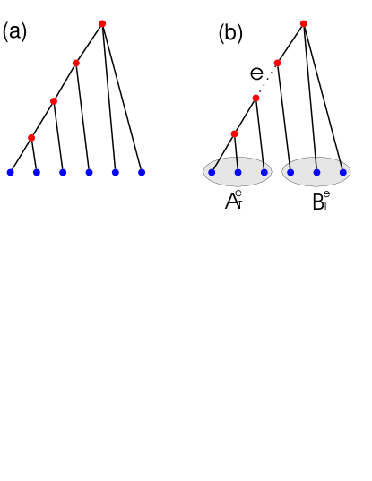
Figure 1: (a) Example of a subcubic tree $T$ with six leaves (indicated in blue). (b) Tree $T\setminus e$ obtained by removing edge $e$ and induced bipartition $(A_{T}^{e},B_{T}^{e})$.

Similarly, one can use the Schmidt rank, i.e., the number of non–zero Schmidt coefficients, instead of the bipartite entropy of entanglement as a basic measure. One then obtains the Schmidt–rank width, or $\chi$–width, denoted by $\chi_{\mbox{\scriptsize{wd}}}(|\psi\rangle)$ [26]. The precise definition is the following. Let $\chi_{A^{e}_{T},B^{e}_{T}}(|\psi\rangle)$ denote the number of non-zero Schmidt coefficients of $|\psi\rangle$ with respect to a bipartition $(A_{T}^{e},B_{T}^{e})$ of $V$ as defined above, i.e. $\chi_{A,B}(|\psi\rangle)={\rm rank}(\rho_{A})$. The $\chi$–width of the state $|\psi\rangle$ is defined by

$$\chi_{\mbox{\scriptsize{wd}}}(|\psi\rangle):=\min_{T}\max_{e\in T}\log_{2}\chi_{A^{e}_{T},B^{e}_{T}}(|\psi\rangle).$$ (13)

Note that, since the inequality

$$\log_{2}\chi_{A,B}(|\psi\rangle)\geq E_{A,B}(|\psi\rangle)$$ (14)

holds for any bipartition $(A,B)$ of the system and for any state $|\psi\rangle$, we have

$$\chi_{\mbox{\scriptsize{wd}}}(|\psi\rangle)\geq E_{\mbox{\scriptsize wd}}(|\psi\rangle).$$ (15)

The entanglement width measures are extensively studied in Refs. [27, 26], to which we refer the interested reader for more details. In particular, it was shown that the Schmidt-rank width can be given a natural interpretation, as this measure quantifies the optimal description of a state in terms of a tree tensor network.

5.2.2 Formulation of the universality criterion

Next we prove that $E_{\mbox{\scriptsize wd}}$ and $\chi_{\mbox{\scriptsize wd}}$ are type II monotones. First we focus on the entropic entanglement width.

Theorem 3.

The entropic entanglement width $E_{\mbox{\scriptsize wd}}(|\psi\rangle)$ is a type II monotone.

Proof: Let $|\phi\rangle$ and $|\phi^{\prime}\rangle$ be two $n$-qubit states, such that $|\phi\rangle$ is (deterministically) convertible by LOCC into $|\phi^{\prime}\rangle$. Let $T_{0}$ be a subcubic tree such that

$$\max_{e\in T_{0}}\ E_{A_{T_{0}}^{e},B_{T_{0}}^{e}}(|\phi\rangle)=E_{\mbox{\scriptsize{wd}}}(|\phi\rangle).$$ (16)

Moreover, let $e_{0}$ be an edge of $T_{0}$ such that

$$E_{A_{T_{0}}^{e_{0}},B_{T_{0}}^{e_{0}}}(|\phi^{\prime}\rangle)=\max_{e\in T_{0}}\ E_{A_{T_{0}}^{e},B_{T_{0}}^{e}}(|\phi^{\prime}\rangle).$$ (17)

We then have:

$$E_{\mbox{\scriptsize{wd}}}(|\phi\rangle) = \max_{e\in T_{0}}\ E_{A_{T_{0}}^{e},B_{T_{0}}^{e}}(|\phi\rangle)$$ (18)

$$\geq E_{A_{T_{0}}^{e_{0}},B_{T_{0}}^{e_{0}}}(|\phi\rangle)$$

$$\geq E_{A_{T_{0}}^{e_{0}},B_{T_{0}}^{e_{0}}}(|\phi^{\prime}\rangle)$$ (19)

$$= \max_{e\in T_{0}}\ E_{A_{T_{0}}^{e},B_{T_{0}}^{e}}(|\phi^{\prime}\rangle)$$ (20)

$$\geq E_{\mbox{\scriptsize{wd}}}(|\phi^{\prime}\rangle).$$ (21)

Further, suppose that $|\psi\rangle$ and $|\psi^{\prime}\rangle$ be $N$-qubit and $n$-qubit states, respectively, such that $|\psi\rangle\geq_{\mbox{\tiny LOCC}}|\psi^{\prime}\rangle$. Then the above implies that

$$E_{\mbox{\scriptsize{wd}}}(|\psi\rangle)\geq E_{\mbox{\scriptsize{wd}}}(|\psi^{\prime}\rangle|0\rangle^{N-n}).$$ (22)

The result is obtained if $E_{\mbox{\scriptsize{wd}}}(|\psi\rangle|0\rangle)=E_{\mbox{\scriptsize{wd}}}(|\psi\rangle)$ for all states $|\psi\rangle$. This is essentially implied by the following property. Suppose that $|\psi\rangle$ is an $N$-qubit state defined on a set of qubits $V:=\{1,\dots,N\}$, and suppose that $|\psi\rangle|0\rangle$ is defined on the set $V^{\prime}:=\{1,\dots,N,N+1\}=V\cup\{N+1\}$. Letting $(A,B)$ be an arbitrary bipartition of $V$ and writing $A^{\prime}:=A\cup\{N+1\}$, we have $E_{A,B}(|\psi\rangle)=E_{A^{\prime},B}(|\psi\rangle|0\rangle).$ This property can straightforwardly be used to show that the entropic entanglement width is the same for the states $|\psi\rangle$ and $|\psi\rangle|0\rangle$. $\square$

Notice, however, that the entropic entanglement width is not a type I entanglement monotone. Despite the fact that (P1) is satisfied, this measure can increase on average under LOCC. This is most easily verified by considering the example of a three-qubit W state [42], from which maximally entangled pairs shared between random pairs of parties can be generated with probability arbitrarily close to one [41]. While the entropic entanglement width of the W state is smaller than one, the entanglement width of the output Bell pairs is equal to one.

An argument similar to the proof of theorem 3 can be used to prove that the Schmidt-rank width also satisfies (P1), i.e., this measure is a type II monotone. In fact, as is e.g. shown in Ref. [43], the Schmidt rank is non-increasing under stochastic local operations and classical communication (SLOCC). It follows that in contrast to the entropic entanglement width, the Schmidt rank width is a type I entanglement monotone, and even satisfies a stronger condition:

Theorem 4.

Consider and $N$-qubit state $|\psi\rangle$ and an $n$-qubit state $|\psi^{\prime}\rangle$ with $N\geq n$, such that $|\psi\rangle$ can be transformed into $|\psi^{\prime}\rangle|0\rangle^{N-n}$ by SLOCC with some non-zero probability. Then $\chi_{\mbox{\scriptsize{wd}}}(|\psi\rangle)\geq\chi_{\mbox{\scriptsize{wd}}}(|\psi^{\prime}\rangle)$. As a corollary, the Schmidt-rank width is a type I and type II monotone.

In order to formulate the criteria for universality associated to the entanglement width measures, we now compute the supremal values of these measures. We will prove that both of these suprema are unbounded, i.e., $E_{\mbox{\scriptsize wd}}^{*}=\chi_{\mbox{\scriptsize wd}}^{*}=\infty$. To obtain these results, it will suffice to show that the entropic entanglement width of the 2D cluster states is unbounded . Notice that the infinity of $E_{\mbox{\scriptsize wd}}$ on the 2D cluster states implies the infinity of $E_{\mbox{\scriptsize wd}}^{*}$. Moreover, the latter implies infinity of $\chi_{\mbox{\scriptsize wd}}^{*}$ via equation (15).

In order to prove that 2D cluster states have an unbounded entropic entanglement width, we need to evaluate this measure on graph states. Here we use a result established in Refs. [27, 26], stating that the entropic entanglement width of a graph state is equal to the rank width of the underlying graph. The rank width is a graph invariant defined in Ref. [45]. One then uses the property that the rank width of the $(2l+1)\times(2l+1)$ grid graph is lower bounded by $l-1$ [46], showing that this measure is indeed unbounded in the limit of infinitely many qubits. This shows that $E_{\mbox{\scriptsize wd}}^{*}=\chi_{\mbox{\scriptsize wd}}^{*}=\infty$.

Combining the above argument with theorems 1, 3 and 4 we arrive at the following criterion for universality.

Theorem 5.

Let $\Psi$ be a universal resource. Then $E_{\mbox{\scriptsize wd}}(\Psi)=\chi_{\mbox{\scriptsize wd}}(\Psi)=\infty.$ Hence, any resource with a bounded $E_{\mbox{\scriptsize wd}}$ or $\chi_{\mbox{\scriptsize wd}}$ cannot be universal.

Although the definitions of the entanglement width measures involve highly nontrivial combinatorial optimization problems, these measures can efficiently be evaluated (or approximated) on several families of states—and hence the corresponding criteria for universality can be employed. In particular, the entanglement width criteria prove to be very powerful to investigate the universality of graph state resources. This is illustrated in the following example.

Example.— It was shown in Refs. [27, 26] that both the entropic entanglement width and the Schmidt-rank width of an arbitrary graph state coincide with the rank width of the underlying graph. Together with theorem 5, this implies that every graph state resource where the rank width of the underlying graphs is bounded, cannot be a universal resource. This criterion leads to many examples of graph state resources which are not universal, as several examples of families of graphs are known where the rank width measure is bounded—in fact, efficient algorithms exists to compute (or approximate) the rank width of any graph [45]. Examples of graphs of bounded rank width, giving rise to non-universal resources, have been given in previous work, see Refs. [27, 26]. These examples include

• tree graphs

• cycle graphs,

• co-graphs,

• graphs locally equivalent to trees,

• distance-hereditary graphs,

• graphs of bounded tree width,

• graphs of bounded clique width,

• …

We refer to the graph theory literature for definitions. Note that two interesting examples of non-universal resources are the linear cluster states (which are instances of tree graphs) and the GHZ states (corresponding to complete graphs), or any family of $k\times l$ lattices where $k$ is constant (and $l$ grows with the system size). $\diamond$

A second application of theorem 5 is obtained by considering ground states of strongly correlated spin systems associated to a one-dimensional geometry.

Example.— Consider ground states of strongly correlated spin systems with nearest-neighbor interaction associated to a one-dimensional geometry. When such systems are in the non-critical phase, one typically finds that the bipartite entropy of entanglement between a subchain of spins and the rest of the chain, is bounded from above by a constant. See e.g. Ref. [47]. For all ground states where this property holds, one can easily show that the entropic entanglement width is bounded. To do so, let $|\psi_{N}\rangle$ be such a ground state of a system of $N$ particles, and consider the subcubic tree $T$ depicted in Fig. 1, where the leaves $1$ to $N$ correspond to the natural linear ordering of the system. As all bipartitions $(A_{T}^{e},B_{T}^{e})$ are such that some connected subchain of particles $\{a,a+1,\dots,a+k\}$ is separated from the rest of the system, one finds that the quantity

$$\max_{e\in T}E_{A_{T}^{e},B_{T}^{e}}(|\psi\rangle)$$ (23)

is bounded from above by a constant (independent of $N$). As (23) is by definition an upper bound to the entropic entanglement width, one finds that this measure is bounded on the resource $\Psi:=\{|\psi_{N}\rangle\}_{N}$. This implies that $\Psi$ cannot be universal. We have therefore found that any resource of ground states of (non-critical) 1D spin systems where the block-wise entanglement entropy is bounded, cannot be a universal resource.

Below (see section 6) we will see that a similar result typically holds for ground states of critical 1D systems, and we will prove that such ground states cannot be efficient universal resources. $\diamond$

5.3 Localizable entanglement

Next we discuss a second class of measures which gives rise to criteria for universality. These measures will be centered around the possibility or impossibility of preparing Bell states by performing LOCC on resource states.

Consider the following simple measure $E_{\mbox{\scriptsize{Bell}}}$: for an arbitrary $N$-qubit state $|\psi\rangle$, define $E_{\mbox{\scriptsize{Bell}}}(|\psi\rangle):=1$ if

$$|\psi\rangle\geq_{\mbox{\tiny LOCC}}\frac{1}{\sqrt{2}}(|00\rangle+|11\rangle),$$ (24)

i.e., if it is possible to deterministically create a Bell pair between a predefined pair of qubits in the system, and $E_{\mbox{\scriptsize{Bell}}}(|\psi\rangle):=0$ if this is not possible. Clearly, one has $E_{\mbox{\scriptsize{Bell}}}^{*}=1$, and $E_{\mbox{\scriptsize{Bell}}}$ is a type II monotone. Therefore, every universal resource $\Psi$ must satisfy $E_{\mbox{\scriptsize{Bell}}}(\Psi)=1$. This is nothing but stating that a universal resource—i.e., a resource capable of preparing arbitrary states—must be able to prepare Bell states, which is a trivial observation. Nevertheless, this this simple criterion allows one to conclude that many resources are not universal. For instance, one can consider the following example.

Example.— The family of W states $\{|W_{N}\rangle\}_{N}$ is not universal, as it has been shown that Bell state cannot be prepared deterministically by performing LOCC on W states [41]. Here we have used the definition

$$|W_{N}\rangle:=\frac{1}{\sqrt{N}}\sum_{i=1}^{N}|e_{N,i}\rangle,$$ (25)

where $|e_{N,i}\rangle$ is defined to be the $N$-qubit computational basis state with a $|1\rangle$-state on the $i$th position in the tensor product, and $|0\rangle$ everywhere else (for example $|e_{3,1}\rangle=|100\rangle$, $|e_{3,2}\rangle=|010\rangle$, …). $\diamond$

Using this idea, a slightly more involved but substantially more powerful criterion can be obtained as follows. Let $|\psi\rangle$ be a state on $N$ qubits $V:=\{1,\dots,N\}$ and let $\alpha$ and $\beta$ be two qubits in the system. Define

$$E^{\alpha,\beta}_{\mbox{\scriptsize{Bell}}}(|\psi\rangle):=1$$ (26)

if it is possible to deterministically create a Bell pair on the qubits $\alpha$ and $\beta$ by performing LOCC on $|\psi\rangle$, and this measure is zero otherwise. Then define the measure ${\cal N}_{\mbox{\scriptsize{LE}}}(|\psi\rangle)$ to be the maximal size $|A|$ of a subset of qubits $A\subseteq V$ such that $E^{\alpha,\beta}_{\mbox{\scriptsize{Bell}}}(|\psi\rangle)=1\mbox{ for all }\alpha\mbox{ and }\beta\mbox{ in }A\mbox{ where }\alpha\neq\beta$. Thus, ${\cal N}_{\mbox{\scriptsize{LE}}}(|\psi\rangle)$ is the largest size of a subset of qubits, such that a Bell state can be created deterministically between any two qubits in this subset, by performing LOCC on $|\psi\rangle$.

It is again clear from the definition that the measure ${\cal N}_{\mbox{\scriptsize{LE}}}$ is a type II monotone. To compute the supremum ${\cal N}_{\mbox{\scriptsize{LE}}}^{*}$, we again consider the 2D cluster states. It is well known that when a system of qubits is in a 2D cluster state, then a Bell pair can be created between any pair of qubits by LOCC [14, 23]. Therefore, ${\cal N}_{\mbox{\scriptsize{LE}}}(|C_{d\times d}\rangle)=d^{2}$, which shows that ${\cal N}_{\mbox{\scriptsize{LE}}}^{*}=\infty$. This leads to the following result.

Theorem 6.

Let $\Psi$ be a universal resource. Then ${\cal N}_{\mbox{\scriptsize{LE}}}(\Psi)=\infty$.

In order to obtain examples of no-go results, we again turn to ground states of strongly correlated spin systems.

Example.— In the context of spin systems, the entanglement measure localizable entanglement, introduced in Ref. [48], is often considered. This measure, which will be connected to ${\cal N}_{\mbox{\scriptsize{LE}}}$, is defined as follows. Let $|\psi\rangle$ be an $N$-qubit state, and let $\alpha$ and $\beta$ denote two arbitrary qubits in the system. The localizable entanglement between these qubits, denoted by $L^{\alpha\beta}(|\psi\rangle)$, is defined to be maximal entanglement (measured by the concurrence) of the subsystem of qubits $\{\alpha,\beta\}$, which can be created on average by performing LOCC on the other qubits in the system. This quantity is an entanglement monotone for $2\times 2\times l$ systems [49] and also fulfills property (P1). Note that $L^{\alpha\beta}$ is maximal (i.e., equal to one) if and only if a Bell pair can deterministically be created between the qubits $\alpha$ and $\beta$ by LOCC—in other words, $L^{\alpha\beta}(|\psi\rangle)=1$ if and only if $E^{\alpha,\beta}_{\mbox{\scriptsize{Bell}}}(|\psi\rangle)=1$. In ground states of strongly correlated spin systems which are organized according to some geometry (such as a $d$-dimensional lattice), $L^{\alpha\beta}$ is typically a decreasing function of the distance between the spins $\alpha$ and $\beta$ [48, 50]. Note that, whenever such a decay law of the localizable entanglement exists, that the measure ${\cal N}_{\mbox{\scriptsize{LE}}}$ must be bounded. This implies that, if the ground state of a spin system exhibits a decay of the localizable entanglement with the distance between spins, then this resource cannot be universal. $\diamond$

Remark 15.

Extension to approximate quasi-deterministic universality.— We note that, contrary to the results obtained for the entanglement width measures, one cannot extend theorem 6 to the case of approximate and/or quasi-deterministic universality (see our upcoming work [36]). Hence, it will be restricted to the case of exact deterministic universality as studied in the present paper. $\diamond$

Remark 16.

Fixed versus random output particles.— Notice that the above arguments are based on the assumption (as already discussed earlier) that the output particles belong to a fixed set $A$ in all branches of the LOCC protocol. If one would allow to generate the desired output state between some, not previously specified, subset of qubits, which might be different for different output branches, the situation changes. As shown in Ref. [41], in this case maximally entangled pairs can be created from the W state quasi-deterministically and one finds that above criteria can no longer be applied. This is true for any “local” measure (such as the localizable entanglement), while “global” measures (e.g., Entropic entanglement width, Schmidt rank width, Schmidt number, Geometric measure of entanglement) can still be used. $\diamond$

5.4 Geometric measure of entanglement

As a third measure we consider the geometric measure of entanglement $E_{g}$, a multipartite entanglement (type I) monotone introduced in Ref. [29], and show that also $E_{g}$ can be used to obtain a criterion for universality. This measure is defined as follows. Let $|\psi\rangle$ be an $N$-qubit state, and let $\pi(|\psi\rangle)$ denote the maximal modulus squared of the overlap between $|\psi\rangle$ and a complete product state on $N$ qubits,

$$\pi(|\psi\rangle)=\max_{|\varphi\rangle=|\varphi_{1}\rangle\otimes\ldots\otimes|\varphi_{N}\rangle}|\langle\psi|\varphi\rangle|^{2}.$$ (27)

Then the geometric measure is defined by

$$E_{g}(|\psi\rangle):=-\log_{2}\pi(|\psi\rangle).$$ (28)

It was proven in Ref. [29] that $E_{g}$ is a type I entanglement monotone. Moreover, this measure trivially satisfies property (ii) stated in theorem 2, i.e., one has $E_{g}(|\psi\rangle|0\rangle)=E_{g}(|\psi\rangle)$. Therefore, one finds that $E_{g}$ is also a type II monotone. In order to compute the supremum $E_{g}^{*}$, we use that the geometric measure of the $d\times d$ cluster states grows as $O(d^{2})$ [51], which implies that $E_{g}^{*}=\infty$. This leads to the following criterion.

Theorem 7.

Let $\Psi$ be a universal resource. Then $E_{g}(\Psi)=\infty$.

Thus, any resource with a bounded geometric measure, cannot be universal.

Example.— The geometric measure of the $N$-qubit W state is equal to [30]

$$E_{g}(|W_{N}\rangle)=(N-1)\log_{2}\frac{N}{N-1},$$ (29)

which, for large $N$, tends to $(\ln 2)^{-1}\sim 1.44$. This shows that $E_{g}$ is bounded for the $W$-states, such that these states can not form a universal resource. $\diamond$

5.5 Schmidt measure

Finally, as a fourth measure we consider the Schmidt measure, a (type I) entanglement monotone introduced in Ref. [28]. The Schmidt measure $E_{s}(|\psi\rangle)$ of an $N$-qubit state $|\psi\rangle$ is defined as the logarithm to base two of the minimal number $K$ of $N$-qubit complete product states $\{|\alpha_{1}\rangle,\dots,|\alpha_{K}\rangle\}$, such that $|\psi\rangle$ can be written as a linear combination

$$|\psi\rangle=\sum_{i=1}^{K}a_{i}|\alpha_{i}\rangle,$$ (30)

for some complex coefficients $a_{i}$. As it can easily be shown that $E_{s}(|\psi\rangle|0\rangle)=E_{s}(|\psi\rangle)$ and as $E_{s}$ is a genuine (type I) entanglement monotone, it follows that the Schmidt measure is a type II monotone. Moreover, one has calculated the Schmidt measure of the 2D cluster states in Ref. [52], yielding $E_{s}(|C_{d\times d}\rangle)=O(d^{2})$, which shows that $E_{s}^{*}=\infty$. We can therefore conclude the following:

Theorem 8.

Let $\Psi$ be a universal resource. Then $E_{s}(\Psi)=\infty$.

Example.— Consider the GHZ states

$$|\psi_{\mbox{\scriptsize{GHZ}}}\rangle:=\frac{1}{\sqrt{2}}\left(|0\rangle^{\otimes n}+|1\rangle^{\otimes n}\right).$$ (31)

By definition, these states have a constant Schmidt measure (equal to $\log_{2}(2)=1$), showing that also by this criterion (see also section 5.2) these states cannot yield universal resource. $\diamond$

6 Efficient universality and scaling of entanglement

In order to obtain criteria for universality, so far we have not considered efficient universality, as defined in section 3.3.2. Evidently, every efficient universal resource must also satisfy theorem 1, and, conversely, any resource which is identified by corollary 2 as not being a universal resource, a fortiori cannot be efficiently universal. However, when efficient universality is taken into account, the criterion in corollary 2 can considerably be strengthened, as we will show in this section.

6.1 General strategy

Our approach will be illustrated by the following example, where we focus on the entropic entanglement width. Consider an efficient universal resource

$$\Psi:=\{|\psi_{1}\rangle,|\psi_{2}\rangle,\dots\},$$ (32)

where $|\psi_{i}\rangle$ is a state on $N_{i}$ qubits, for every $i=1,2,\dots$. For every $d\times d$ cluster state on $n=d^{2}$ qubits, there exists a state $|\psi_{f(n)}\rangle\in\Psi$ in the resource $\Psi$ (where $f(n)\in\{1,2,\dots\}$), such that $|\psi_{f(n)}\rangle\geq_{\mbox{\tiny LOCC}}|C_{d\times d}\rangle$, thus showing that

$$E_{\mbox{\scriptsize wd}}(|\psi_{f(n)}\rangle)\geq E_{\mbox{\scriptsize wd}}(|C_{d\times d}\rangle)\geq O(\sqrt{n}).$$ (33)

In the last equality we have used that the rank width of the $(2l+1)\times(2l+1)$ grid graph is larger then $l-1$, as proven by Oum [46]. This implies that the entropic entanglement width of the $d\times d$ cluster states scale (at least) as $O(d)=O(\sqrt{n})$. As $\Psi$ is an efficient universal resource, the number of qubits $N_{f(n)}$ on which $|\psi_{f(n)}\rangle$ is defined, only grows polynomially with the size $n$ of the 2D cluster states (see observation 3 in section 4.2). Thus, there exists a polynomial $p(n)$ such that $N_{f(n)}\leq p(n)$. Conversely, for large $n$ (where we only consider the leading order, denoted by $k$, of the polynomial $p(n)$), one has $n\geq O((N_{f(n)})^{1/k})$, thus showing that

$$E_{\mbox{\scriptsize wd}}(|\psi_{f(n)}\rangle)\geq O((N_{f(n)})^{1/(2k)}).$$ (34)

We therefore find a necessary condition on the scaling behavior of the entanglement measure $E_{\mbox{\scriptsize wd}}$ on any efficient universal resource $\Psi$: equation (34) shows that $E_{\mbox{\scriptsize wd}}(|\psi_{i}\rangle)$ must grow as $O((N_{i})^{1/(2k)})$ for some $k$, which is essentially equivalent to stating that this measure must grow faster-than-logarithmically with the system size on $\Psi$. Hence, resources where the entropic entanglement width grows at most as the logarithm of the system size, cannot be efficient universal resources (in particular, resources with bounded entanglement width are covered by this result).

The argument of the above example can be repeated for all type II monotones $E$. In every case, a necessary condition on the scaling behavior of $E$ for efficient universal resources is obtained. More formally, one has the following.

Theorem 9.

Let $\Psi:=\{|\psi_{1}\rangle,|\psi_{2}\rangle,\dots\},$ be a resource, where $|\psi_{i}\rangle$ is a state on $N_{i}$ qubits, for every $i$. Let $E$ be a type II monotone, and let $\varphi$ be a function such that, for every 2D cluster state $|C_{d\times d}\rangle$ on $n=d^{2}$ qubits, one has

$$E(|C_{d\times d}\rangle)\geq\varphi(n).$$ (35)

If $E(|\psi_{i}\rangle)$ scales as $\log\varphi(N_{i})$, then $\Psi$ cannot be an efficient universal resource.

This result should be regarded as a strengthening of theorem 1. We emphasize again that the 2D cluster states in principle do not play a distinguished role in theorem 9, in the sense that they can be replaced—without weakening or strengthening the result—by arbitrary efficient universal resources or, in fact, any family of states which themselves also can efficiently be prepared. However, as pointed out before, being graph states, the 2D cluster states usually form a suitable test-bed also in this case.

Specializing these considerations to entanglement width, localizable entanglement, geometric measure and Schmidt measure, one finds:

Theorem 10.

Let $\Psi$ be a resource. If one of the measures $E_{\mbox{\scriptsize wd}}$, $\chi_{\mbox{\scriptsize wd}}$, ${\cal N}_{\mbox{\scriptsize{LE}}}$, $E_{g}$ or $E_{s}$ scales at most logarithmically with the system size on $\Psi$, then $\Psi$ cannot be an efficient universal resource.

The proof of this result simply follows from the fact that all these measures scale as $O(n^{1/k})$, for some $k$, for the 2D cluster states on $n$ qubits.

When considering entanglement width, the above criterion allows one to determine new examples of no-go results which were not detected by theorem 1.

Example.— Consider, as at the end of section 5.2.2, a family of ground states $\{|\phi_{N}\rangle\}$ of a 1D spin system, where $|\phi_{N}\rangle$ is a state of $N$ spins. Investigating now the critical phase, one typically has that the block entanglement entropy of a subchain of spins of length $L\leq N$ scales as $\log L$ [47]. Similar to the example in section 5.2.2, one then finds that the entanglement width of such a ground state can at most scale as the logarithm of the system size. This shows that any resource of ground states of 1D (critical) spin systems where the block entanglement of a subchain scales as the logarithm of the length of the subchain, cannot be an efficient universal resource. Thus, together with the example in section 5.2.2, we find that ground states of critical or non-critical 1D spin systems can typically not be efficient universal resources. $\diamond$

Another interesting no-go result is obtained using the Schmidt measure.

Example.— One easily finds that the Schmidt measure can grow at most logarithmically with the system size for the W states (this immediately follows from the definition of these states). This implies that the W states cannot be efficient universal resources. In contrast to the argument based on localizable entanglement (see also section 5.3), the argument presented here is also valid when considering the possibility of random output particles. Note also that by considering the geometric measure, as in section 5.4, one can conclude that the W states do not form an (efficient) universal resource. $\diamond$

6.2 Efficient universality and classical simulation of MQC

It is instructive to point out a relation between efficient (exact deterministic) universality of a resource $\Psi$ and the problem of efficiently (i.e., with polynomial overhead) classically simulating MQC on this resource. When a resource is identified as not being an efficient universal resource, one may wonder whether an efficient classical simulation of MQC on this resource becomes possible. Although one can of course not expect that such a result would hold in general, here we note that such a property is valid if one considers the criteria for efficient universality corresponding to the Schmidt-rank width and the Schmidt measure. In particular, in previous work [26] we showed that MQC can be simulated on every resource where the Schmidt-rank width grows only logarithmically with the system size. This shows that any resource which is ruled out by the Schmidt-rank width criterion in theorem 9 as an efficient universal resource, allows an efficient classical simulation of MQC.

A similar remark can be made regarding the Schmidt measure. Suppose that $\Psi$ is a resource where the Schmidt measure grows at most logarithmically with the system size. Equivalently, every state in the family $\Psi$ can be written as a linear combination of polynomially many (w.r.t. the number of qubits) complete product states. One then easily verifies that any LOCC on such states can be simulated with polynomial overhead by a classical computer. In particular, the expectation value of a local observable $O:=O_{1}\otimes\dots\otimes O_{n}$ can be efficiently computed when an $n$-qubit system is in a state $|\psi\rangle$ with logarithmically scaling Schmidt rank: writing

$$|\psi\rangle=\sum_{i=1}^{K}a_{i}|\alpha_{i}\rangle,$$ (36)

where the $\{|\alpha_{i}\rangle\}$ are $K=$ poly$(n)$ complete product states, the expectation value

$$\langle\psi|O|\psi\rangle=\sum_{i,j=1}^{K}a_{i}\bar{a}_{j}\langle\alpha_{i}|O|\alpha_{j}\rangle$$ (37)

can efficiently be computed, as every term $\langle\alpha_{i}|O|\alpha_{j}\rangle$ can be efficiently computed and as there are only poly$(n)$ such terms in the above sum. Similarly, a state obtained after performing a local projection on $|\psi\rangle$ can efficiently be determined (note that such states can have a Schmidt measure of at most $\log_{2}K$). One can therefore conclude that any resource which fails to pass the Schmidt measure criterion in theorem 9, even allows an efficient classical simulation of MQC.

Thus, it is interesting to find that in the issue of efficient universality, as well as in the context of efficient simulation of MQC, the scaling of entanglement with the system size plays an important role.

7 Examples of efficient universal resources

To provide examples of universal resource states, our strategy is to establish an equivalence, up to a polynomial overhead, among (efficient) universal resources. The proof of efficient universality of the 2D cluster states [5, 6] means an efficient capability to simulate any circuit model by LOCC and, in particular, to prepare any other resource state by LOCC. Thus, all we have to show for other resource states is that the opposite transformation is also efficiently possible.

Theorem 11.

The graph states corresponding to the 2D square, hexagonal, triangular and Kagome lattices are efficient universal resources for MQC.

Proof: According to our strategy, a proof is given in the form of an explicit deterministic LOCC protocol which transforms such other candidate states into the 2D cluster state with a polynomial overhead in resources and operations (see Fig. 2).

As LOCC, we translationally apply $\sigma_{y}$ and $\sigma_{z}$ measurements, which are known to correspond to simple update rules of the graph, namely local complementation (inversion of the neighborhood subgraph) and vertex deletion, respectively [23]. We will get a resulting graph state deterministically after applying local Clifford unitary corrections $u_{y,k}$ and $u_{z,k}$ on neighboring qubits (with help of classical communication), such as

$$u_{y,k} = \sqrt{(-1)^{k}(-i\sigma_{z})}=\frac{1}{\sqrt{2}}\left({\bf 1}-(-1)^{k}i\sigma_{z}\right),$$

$$u_{z,k} = \sigma_{z}^{k},$$

which depend on the measurement outcomes $k=\{0,1\}$.

Let us illustrate such graph transforms to prove the theorem. Our LOCC protocol transforms (a) hexagonal-lattice graph state into (d) the 2D cluster state via (b) the triangular-lattice and (c) the Kagome-lattice graph state sequentially. When we apply the $\sigma_{y}$ measurements on vertices of the hexagonal lattice in Fig. 2  (a), we will have a triangle around the measured qubits by the local complementation. The resulting graph turns out to be a triangular lattice (b). Next, we apply the $\sigma_{z}$ measurements on vertices marked by $\diamond$, which simply deletes the measured qubits along with the attached edges. The graph now becomes a so-called Kagome lattice, which has degree 4 uniformly in a similar manner as the square lattice. The last step is a bit involved, but straightforward by applying $\sigma_{y}$ and $\sigma_{z}$ measurements according to the ordering of Fig. 2. Accordingly, we finally obtain a square lattice, i.e., a 2D cluster state. The total spatial overhead is eight in that a unit square on (d) is obtained from eight hexagons in (a). Since the overhead is constant, all resource states are efficient universal. $\square$

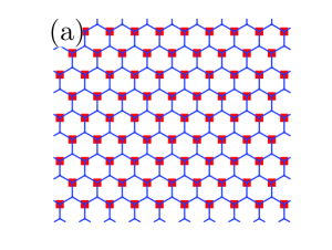
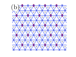
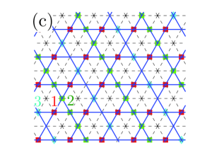
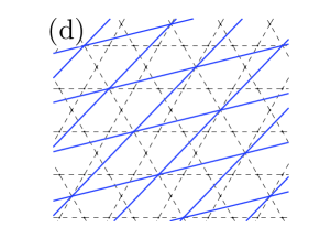
Figure 2: Examples of efficient universal resource for MQC. These are graph states corresponding to (a) hexagonal, (b) triangular and (c) Kagome lattices. Deterministic LOCC transformation from (a) to (d) (2D cluster state) via (b) and (c) is indicated, where simple graph rules can be used sequentially ($\sigma_{y}$ and $\sigma_{z}$ measurements are displayed by $\square$ and $\diamondsuit$, respectively). The spatial overhead for the transformation is constant.

Note that, since these other resource states can be transformed into the 2D cluster state always by adaptive local projective measurements assisted with classical communication, and local (Clifford) operations, they are also universal in the sense of a conventional one-way quantum computation.

It is interesting to observe that the square lattice, together with the hexagonal and triangular lattices are the only possibilities to obtain a regular tiling of the 2D plane. Furthermore, the Kagome lattice is an example of a uniform semiregular 2D tiling with 2 basic tiles (the triangle and the hexagon). The hexagonal lattice has vertex degree 3, which leads to an increased robustness against local noise as compared to the 2D cluster state [53]. Since the 1D cluster state (with uniform vertex degree 2) has been proved not to be universal [27], the vertex degree 3 is minimal for universal resource on uniform lattice structures.

We remark that other universal resource states have been presented [54] based on non-uniform lattice structures (see also [55]), where each gate in a universal set of unitary gates can be implemented by local measurements on an elementary unit and these units are combined (bottom-up approach). Here we took, in contrast, a top–down approach, where we prove universality by explicitly constructing LOCC protocols that yield the 2D cluster state.

Of course, we can simulate directly any circuit model on such new universal resources in practice, without transforming them into the 2D cluster state of the 2D square lattice. Let us illustrate this by a hexagonal lattice (due to its potential advantage for the local decoherence compared with a square lattice). In Fig. 3, we show a direct simulation of the circuit model on the 2D hexagonal lattice, after deleting uncolored qubits by the $\sigma_{z}$ measurements. We consider each snaking horizontal path running from the left to the right as a quantum wire which corresponds to an evolution of a logical single qubit in the circuit model.

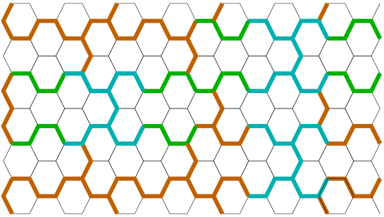
Figure 3: A direct simulation of the circuit model on the hexagonal lattice. After measuring uncolored qubits in the $\sigma_{z}$ direction, the resource state is capable of simulating a set of universal gates between any neighboring two quantum wires (snaking horizontal paths) and to compose them into an arbitrary unitary operation. Here we illustrate an implementation (with the same measurement pattern of Ref. [5, 6]) of CNOT and of arbitrary $SU(2)$ rotation with the Euler decomposition by the 15-qubit 90-degree rotated H part (blue) and the 5-qubit chain part (green), respectively.

Here we give an alternative proof of its efficient exact deterministic universality in a similar manner as the proof of the 2D cluster state [5, 6] (see also Ref. [54] for other resources). Namely, we take a bottom-up approach by showing two (sufficient) conditions are fulfilled for our family of resource states:

• Simulation of a universal set of elementary gates: It is capable of implementing a set of universal gates on logical qubits with at most polynomial overhead.

• Composability: The simulation (i) of elementary gates is composable between any neighboring pair of logical qubits, as well as repeatable.

Here we follow the implementation (measurement pattern) of Ref. [5, 6] of CNOT and of arbitrary $SU(2)$ rotation with the Euler decomposition in terms of the 15-qubit 90-degree rotated H part (blue) and the 5-qubit chain part (green), respectively. The capability of implementing such gates as often as required follows immediately from its periodic structure. The length of an extra one-dimensional path can be adjusted, if necessary, by the $\sigma_{y}$ measurement.

A slightly more economical simulation can also be done by selecting the controlled-phase gate and the set $SU(2)$ of single-qubit rotations as a set of elementary gates for the circuit model. By measuring the middle qubit of the “bridge between quantum wires” (i.e., the center qubit in the blue part) in the $\sigma_{y}$ direction, we can simply implement a logical “remote” controlled-phase gate (cf. Ref. [54]), without additional measurements along the quantum wires.

8 Encoded universality

So far we have restricted our attention to situations where the resource states consist of systems with fixed dimension $d$, and where the desired target states are multipartite states of $d$-dimensional systems. We have concentrated on $d=2$, i.e., qubit systems, and have provided definitions and criteria when such a family of resource states is capable of producing any other quantum state of $n$ qubits. In this section we will show how to extend our results in order to take higher-dimensional systems, generation of systems with different dimensions, and encoded quantum states into account. We will first specify what we mean by encoding, and then put forward a definition for encoded (CQ-)universality in MQC, based on different notions of locality. We will finally discuss the applicability of entanglement criteria developed in the previous sections, and discuss examples of encoded universal resources.

8.1 Encoded quantum states

We start by some general considerations on encoded quantum states.

8.1.1 Qubits and qudits

In the measurement-based model for quantum computation, a resource state constituting of $N$ two-dimensional systems is processed by sequences of LOCC. It is clear that the physical systems remain the same throughout the procedure, and hence the resulting quantum state is also one consisting of qubits. It is impossible to generate a state of $d$-dimensional systems (qudits) from a qubit system. More generally, if the system constituting the resource state are $k$-dimensional, and the states to be generated constitute of $d$-dimensional systems, then one cannot generate any such state whenever $k\not=d$. What is, however, possible, is to generate the desired state in an encoded form. In almost all conceivable cases, the generation of a quantum state in such an encoded form is sufficient.

The most natural kinds of encoding are the following:

• If $k\geq d$, then ideally one encodes $m=\lfloor\log(k)/\log(d)\rfloor$ $d$-level systems into one $k$–level system.

• If $k<d$, then ideally one uses $m=\lceil\log(d)/\log(k)\rceil$ $k$-level system to encode one $d$-level system.

In neither of these two cases additional levels are used. One may also consider more complex encodings, e.g., any encoding that can be generated by a poly-sized quantum circuit. However, in this case quantum information corresponding to a $d$-level system may be distributed among all $k$-level systems. In the following, we will restrict ourselves to the kinds of encodings specified above, where a natural association with physical systems is maintained. This restriction allows us to use entanglement-based criteria for universality also for encoded systems.

8.1.2 General encodings

The treatment of systems of different dimensionality is not the only case where encodings are useful. Even if one is restricted to qubits, it is natural to consider the question whether states can be generated in an encoded way. Encoded states appear naturally in, e.g., quantum computation once error-correction is considered. In particular, any fault-tolerant implementation of quantum computation actually generates states in an encoded form, and performs unitary operations on the encoded states. In this case the (redundant) encoding serves to protect quantum information against the influence of errors. One may consider encodings also for different reasons. For instance, for certain physical set-ups it may be impossible (or very hard) to perform arbitrary single-qubit operations and two-qubit gates. However, for certain encodings the implementation of logical single- and two-qubit gates, i.e., gates acting on the encoded or logical systems, is possible. Such a situation occurs for instance in charge-controlled quantum dots, where despite of difficulties to obtain inhomogeneous single-spin rotations, processing of encoded quantum information is possible [56, 57, 58]. Finally—and this brings us back to the present study of universality—if one is ultimately interested in a CC computational scheme, it is often sufficient that a quantum computer is capable of generating states in an encoded form. In particular, we will see below that any encoded CQ-universal resource for MQC is also CC-universal.

For simplicity, in the following we will restrict ourselves to the case where $k=d=2$. Generalization to $k\not=d\geq 2$ is, however, straightforward.

Next we define what is meant by “encoded qubits” and “encoded quantum states”. First we consider encodings of one-qubit systems and states.

Definition 3.

(Encoded qubit): An $m$-qubit encoding ${\cal E}:=({\cal H},\{|{\bm{0}}\rangle,|{\bm{1}}\rangle\})$ of a one-qubit system is specified by

• a Hilbert space ${\cal H}\cong\mathbb{C}^{2^{m}}$, representing a system of $m$ qubits, and

• two (fixed) orthogonal states $|\psi_{0}\rangle,|\psi_{1}\rangle\in{\cal H}$. We use the shorthand notation $|{\bm{0}}\rangle:=|\psi_{0}\rangle\mbox{ and }|{\bm{1}}\rangle:=|\psi_{1}\rangle.$

Let $|\phi\rangle=a|0\rangle+b|1\rangle$ be an arbitrary one-qubit state. The encoded version of $|\phi\rangle$ with respect to the encoding ${\cal E}$ is the state $|{\bm{\phi}}\rangle:=a|\bm{0}\rangle+b|\bm{1}\rangle\in{\cal H}$.

This definition is now generalized to encompass encodings of many-qubit systems and states.

Definition 4.

(Encoded $n$-qubit system): An $m$-qubit encoding ${\cal E}:=({\cal H}^{E},{\cal P},\{|{\bm{0}}\rangle,|{\bm{1}}\rangle\})$ of an $n$-qubit system is specified by

• a Hilbert space ${\cal H}^{E}\cong\mathbb{C}^{2^{mn}}$, representing a system of $m\cdot n$ qubits labeled by a set $E=\{1,\dots,m\cdot n\}$,

• a partition ${\cal P}:=\{A_{1},\dots,A_{n}\}$ of $E$, where every $A_{k}$ denotes a set of $m$ qubits of $E$, and

• two (fixed) orthogonal $m$-qubit states $\{|{\bm{0}}\rangle,|{\bm{1}}\rangle\}$.

Consider an $n$-qubit state

$$|\phi\rangle=\sum_{i_{1},i_{2},\ldots i_{n}\in\{0,1\}^{n}}c_{i_{1}i_{2}\ldots i_{n}}|i_{1}\rangle|i_{2}\rangle\ldots|i_{n}\rangle.$$ (38)

The encoded version of $|\phi\rangle$ w.r.t. the encoding ${\cal E}$ is the state

$$|{\bm{\phi}}\rangle=\sum_{i_{1},i_{2},\ldots i_{n}\in\{0,1\}^{n}}c_{i_{1}i_{2}\ldots i_{n}}|{\bm{i}_{1}}\rangle_{A_{1}}|{\bm{i}_{2}}\rangle_{A_{2}}\ldots|{\bm{i}_{n}}\rangle_{A_{n}}\in{\cal H}^{E}.$$

Here the subscripts $A_{k}$ denote on which qubits the states $|{\bm{i}}_{k}\rangle$ are defined.

For notational simplicity, in the definition above we have considered the same encoding for every qubit. Generalization to different encodings for different qubits is straightforward.

Similarly, for $k\not=d\geq 2$ an encoded qudit can be defined by a set of $d$ orthogonal states of $m$ $k$-level systems, and the definition of an encoded state follows immediately. The case of generating $d$-level systems using $k$-level systems is also covered, where the encoding corresponds to (i) or (ii) specified in Sec. 8.1.1.

8.2 Local operations on encoded systems

The notion of locality is central in MQC. In particular, entangled quantum states are processed by local operations and classical communication. This allows one to attribute entanglement as a resource to the initial state of the system, and only in this context criteria based on entanglement properties of resource states as presented in section 5 become meaningful. When considering systems with a fixed dimension, e.g., qubits, as we did in the previous sections, the notion of locality is unique and simply corresponds to single-qubit operations. When considering encoded systems as we do here, one may, however, consider two different notions of locality, and the corresponding classes of “local” operations assisted by classical communication.

• Local with respect to physical systems constituting the resource state: LOCC

• Local with respect to the encoded systems: LOCC

It depends on the context at hand which of these two notions of locality is of interest. The first notion, associating locality to the physical systems constituting the quantum state, seems to be the most natural one. However, in some cases one might also naturally consider (ii), i.e., locality with respect to logical or encoded system. Notice that in the case of LOCC, joint operations on certain groups of physical qubits are allowed. Hence, if we consider LOCC in the definition for universality, we obtain a more stringent requirement as when using LOCC. Usage of LOCC will turn out to be useful when considering entanglement-based criteria for encoded universality.

8.3 Definition of encoded universality

In this section, we precisely define what is meant by an “encoded universal resource for MQC”. In order to do so, we first need to specify the notion of a “consistent family of encodings”, which is the following. In the present study, the role of an infinitely large resource is played by a family of states $\Psi=\{|\psi_{1}\rangle,|\psi_{2},\rangle,\dots\}$, where $|\psi_{i}\rangle$ is a state on $N_{i}$ qubits and where $N_{i}\leq N_{i+1}$ for every $i$. More precisely, the state $|\psi_{i}\rangle$ belongs to a Hilbert space ${\cal H}^{E_{i}}$, where $E_{i}$ denotes a set of $N_{i}$ qubits, such that $E_{i}\subseteq E_{i+1}$, for every $i$. We will say that $\{{\cal H}^{E_{1}},{\cal H}^{E_{2}},\dots\}$ is a nested family of Hilbert spaces. Now, suppose that, for every Hilbert space ${\cal H}^{E_{i}}$ an encoding ${\cal E}_{i}=\{{\cal H}^{E_{i}},{\cal P}_{i},\{|\bm{0}\rangle,|\bm{1}\rangle\}\}$ is given. Since a resource $\Psi$ plays the role of an infinitely large state, when considering encodings—together with the corresponding partitions of the systems ${\cal H}^{E_{i}}$ into logical qubits as specified by the encodings ${\cal E}_{i}$—it is natural to impose a certain degree of consistency of these encodings. In particular, we will require that the way in which the Hilbert space ${\cal H}^{E_{i}}$ is partitioned into logical qubits, should be consistent with the way in which ${\cal H}^{E_{i+1}}$ is partitioned, i.e., ${\cal P}_{i}\subseteq{\cal P}_{i+1}$ for every $i$. In such case, we will call ${\cal F}:=\{{\cal E}_{1},{\cal E}_{2},\dots\}$ a consistent family of encodings.

We are now in a position to give a definition of encoded universal resource for MQC.

Definition 5.

(Encoded universality): Consider a nested family of Hilbert spaces $\{{\cal H}^{E_{i}}\}_{i}$, and let $\Psi=\{|\psi_{1}\rangle,|\psi_{2}\rangle,\dots\}$ be a family of states such that $|\psi_{i}\rangle\in{\cal H}^{E_{i}}$, for every $i$. Let ${\cal F}:=\{{\cal E}_{1},{\cal E}_{2},\dots\}$ be a consistent family of $m$-qubit encodings of this family of Hilbert spaces. The family $\Psi$ is called an encoded universal resource for MQC with respect to ${\cal F}$, if for every $n$ and for every $n$-qubit quantum state $|\phi_{\rm out}\rangle$, there exists a state $|\psi_{i}\rangle\in\Psi$ such that $|\psi_{i}\rangle\geq_{\mbox{\tiny LOCC}}|\bm{\phi}_{out}\rangle$, where $|{\bm{\phi}}_{out}\rangle$ is the encoded version of $|\phi_{out}\rangle$ w.r.t. the encoding ${\cal E}_{i}$.

The family $\Psi$ is said to be an encoded universal resource for MQC if there exist a consistent family of encodings with respect to which $\Psi$ is universal.

Remark 17.

General comments regarding definition 5.—

(i) Any resource that is universal is also encoded universal, although the opposite is not necessarily true. We will discuss examples for such cases later in this section.

(ii) Although we allow for an arbitrary one-qubit encoding, the encoding needs to be fixed, i.e., it needs to be the same for all output states.

(iii) As in the case of non-encoded universality, we also assume here that the output state is prepared on the same output particles in all branches of the LOCC protocol (an extension to random output particles is possible in the same way as in the non-encoded case).

(iv) In definition 5 we refer to LOCC, i.e., operations on the individual physical systems (see (i) in the preceding section). One may also consider a weaker form of universality with respect to LOCC.

(v) In the above definition, the same encoding is used for every qubit. This restriction can easily be lifted without changing the results to be presented in the following. We have adopted this version of the definition for notational convenience.

(vi) In this paper we do not consider general encodings by means of arbitrary poly-sized quantum circuits. This is a restriction in the sense that the latter leads to a more general definition of encoded universality (i.e., it is likely that there exist encoded universal resources w.r.t. such general codings which are not covered by the present theory). The reason for this is that it is not clear how criteria stated in terms of entanglement can be formulated for such general encodings, whereas this will be possible for the current definition. However, it is clear that general encodings by poly-sized quantum circuits deserve further attention. $\diamond$

We will sometimes consider a slightly weakened version of encoded universality, in the following sense. Let $\{|\bm{0}\rangle,|\bm{1}\rangle\}$ be an ($m$-qubit) encoding of a one-qubit system, let $|\bm{\phi}\rangle$ be an encoded version of an $n$-qubit state $|\phi\rangle$ with respect to this encoding (see definition 5), and let $U=U_{1}\otimes\dots\otimes U_{n}$ be an $n$-qubit local operation, where

$$U_{k}:=a|0\rangle\langle 0|+b|0\rangle\langle 1|+c|1\rangle\langle 0|+d|1\rangle\langle 1|$$ (39)

(for every $k=1,\dots,n$). Then the encoded version ${\bm{U}}={\bm{U}}_{1}\otimes\dots\otimes{\bm{U}}_{n}$ of this operator is defined by

$${\bm{U}}_{k}:=a|\bm{0}\rangle\langle\bm{0}|+b|\bm{0}\rangle\langle\bm{1}|+c|\bm{1}\rangle\langle\bm{0}|+d|\bm{1}\rangle\langle\bm{1}|,$$ (40)

and naturally acts as

$${\bm{U}}|\bm{\phi}\rangle=\sum_{{i_{1},i_{2},\ldots i_{n}=0}}^{1}c_{i_{1}i_{2}\ldots i_{n}}{\bm{U}}_{1}|{\bm{i}_{1}}\rangle_{A_{1}}\ldots{\bm{U}}_{n}|{\bm{i}_{n}}\rangle_{A_{n}}.$$

For example, given an encoding $\{|\bm{0}\rangle,|\bm{1}\rangle\}$ the logical single-system Pauli operations are defined by

$${\bm{\sigma}_{z}}=|\bm{0}\rangle\langle\bm{0}|-|\bm{1}\rangle\langle\bm{1}|,$$

$${\bm{\sigma}_{x}}=|\bm{0}\rangle\langle\bm{1}|+|\bm{1}\rangle\langle\bm{0}|,$$ (41)

$${\bm{\sigma}_{y}}=-i|\bm{0}\rangle\langle\bm{1}|+i|\bm{1}\rangle\langle\bm{0}|.$$

Note that an operation which is local in the sense of logical qubits need not be local at the level of the physical qubits in the system, i.e., it may act jointly on several physical qubits.

We will sometimes consider resources which are encoded universal in the restricted sense that it is possible to prepare an encoded version of any state up to logical local operations. Notice that a resource which is universal in this (restricted) sense with respect to CQ is, however, fully CC-universal. That is, if we are only interested in obtaining classical outputs, such logical local operations do not play a role as we simply have to adapt the basis of the final measurements. We also note that the 2D cluster states are CQ-universal under projective local measurements up to Pauli operations; this property, together with the above restricted notion of encoded universality, will play a role in the next section.

8.4 Encoded universality and the 2D cluster states

In this section, it is our aim to relate encoded universal resources to (encoded versions of) the “standard” universal resource, the family of 2D cluster states, i.e., this section will contain a result analogous to observation 1 in section 4. Although this result will be highly analogous to observation 1, its proof will not be as straightforward and will require some extra work. The result is the following.

Theorem 12.

A family of states $\Psi$ is an encoded universal resource with respect to a specific encoding (more precisely: w.r.t. a consistent family of encodings) up to logical Pauli operators, if and only if encoded 2D cluster states $|\bm{C}_{d\times d}\rangle$ of arbitrary size $d$ with respect to the same encoding can be generated by means of LOCC, up to logical Pauli operations.

A family of states $\Psi$ is an encoded universal resource up to logical Pauli operators if and only if there exists an encoding (more precisely: a consistent family of encodings) such that encoded 2D cluster states $|\bm{C}_{d\times d}\rangle$ of arbitrary $d$ can be generated by means of LOCC, up to logical Pauli operations.

Proof: Necessity of the condition is obvious, as an encoded universal resource must be capable of producing an encoded version of any state, in particular an encoded 2D cluster state. Sufficiency of the condition is based on the fact that an encoded 2D cluster state is an encoded universal resource under LOCC up to logical Pauli operations for any encoding. The proof of the latter statement is postponed until Theorem 16. $\square$

Note that it is by no means trivial that local operations on physical qubits allow one to process encoded quantum information. E.g., as already indicated above, logical local operations need not act locally on the physical qubits, i.e., one may not be able to realize logical local operations as physical local operations. For example, consider a 3-qubit encoding where $|\bm{0}\rangle:=|000\rangle$ and $|\bm{1}\rangle:=|W_{3}\rangle$, where the latter is the W state on 3 qubits. It is clear that in this case a logical $\sigma_{x}$ operation, i.e.,

$${\bm{\sigma}}_{x}:=|000\rangle\langle W_{3}|+|W_{3}\rangle\langle 000|$$ (42)

acts non-locally on the physical qubits.

However, we will find that it is always possible to realize logical projective two-outcome measurements (which are the basic ingredient of the one-way 2D cluster state model) by physical local operations. We again refer to Theorem 16.

8.5 Criteria for universality

We have discussed entanglement-based criteria for non-encoded universality in Sec. 5 and 6. Here we discuss to which extent these criteria can be applied—either directly or in an adapted form—in the context of encoded universality .

8.5.1 Criteria at the level of encoded systems

The first observation is that one can use exactly the same criteria for universality when considering encoded universality, if one applies them at the level of encoded systems. This is expressed in the following

Theorem 13.

Consider a fixed (consistent family of) encoding(s), which also implies a partition of the system. Any entanglement-based criterion for universality formulated for non-encoded systems using LOCC leads to a criterion for the encoded system by considering the corresponding entanglement measures where locality is defined with respect to the partition of the system, i.e., LOCC.

The proof of this theorem is straightforward, as one can treat any logical qubit as a two–level system if LOCC are allowed.

Remark 18.

Entanglement with respect to partitions.— For a fixed encoding, one considers local operations with respect to this encoding, i.e. LOCC. Entanglement is defined relative to the partitions induced by the encoding. For instance, one says that $E_{\rm Bell}(|\bm{\phi}\rangle)=1$ if an encoded entangled pair $(|{\bm{0}}\rangle|{\bm{0}}\rangle+|{\bm{1}}\rangle|{\bm{1}}\rangle)/\sqrt{2}$ can be created between some pair of encoded systems. In case of entanglement width measures, they are now defined with respect to the fixed partition. That is, entanglement between blocks of qubits is considered, where each block consists of several physical qubits specified by the encoding. Entanglement within each block is irrelevant and absorbed into the encoding. Notice that in this way one still obtains a set of powerful criteria to assess whether a given state is encoded universal with respect to a fixed encoding. In particular, any encoded universal resource still needs to have unbounded entanglement width (defined via LOCC). $\diamond$

Remark 19.

Simultaneous treatment of different encodings.— Notice that above criterion automatically provides a test for all encodings that lead to the same partition of the system, i.e. the same notion of LOCC, independent of the choice of the two orthogonal states constituting the logical qubit. However, it would still be desirable to obtain a more general statement about non-universality with respect to all possible encodings. Although many encodings are treated simultaneously, one still needs to check for all possible partitions of the system and determine the corresponding measures, which is impractical. $\diamond$

In the following, we utilize entanglement-based criteria at the level of physical systems to infer statements about encoded universality. This turns out to be possible, although only under certain circumstances and for certain entanglement measures.

8.5.2 Schmidt measure and geometric measure

In this section, we will show that every encoded universal resource must have an unbounded Schmidt measure and geometric measure, i.e., $E_{s}(\Psi)=\infty=E_{g}(\Psi)$ for every encoded universal resource $\Psi$.

We start by considering the geometric measure. Let $|\psi\rangle$ be a state defined on a set of qubits $S:=\{1,\dots,n\}$, and let ${\cal P}:=\{A_{1},\dots,A_{l}\}$ be any partition of the set $S$ into $l$ subsets $A_{i}$. One can regard $|\psi\rangle$ as an $l$-party state, where every subset $A_{i}$ is associated to a party. At this coarse-grained level one can also define the geometric measure $E_{g}^{\cal P}$ in a natural way, where now locality is defined with respect to these $l$ parties. An important property is now that $E_{g}^{\cal P}(|\psi\rangle)\leq E_{g}(|\psi\rangle)$ for any partition ${\cal P}$, i.e., the geometric measure is non-increasing under coarsening of the partition [28].

This property will be crucial for proving that $E_{g}(\Psi)=\infty$ for every encoded universal resource $\Psi$. Let $\{|{\bm{0}}\rangle,|{\bm{1}}\rangle\}$ be an $m$-qubit encoding with respect to which $\Psi$ is encoded universal, and let $|\phi\rangle=\sum c_{i_{1}\dots i_{n}}|i_{1}\dots i_{n}\rangle$ be an arbitrary $n$-qubit state. By the encoded universality of $\Psi$, there exists a state $|\psi_{i}\rangle\in\Psi$ and an encoded version $|\bm{\phi}\rangle$ of $|\phi\rangle$ such that $|\psi_{i}\rangle\geq_{\mbox{\tiny LOCC}}|\bm{\phi}\rangle$. As $E_{g}$ is a type II entanglement monotone, this implies that $E_{g}(|\psi_{i}\rangle)\geq E_{g}(|\bm{\phi}\rangle)$. Let $S:=\{1,\dots,m\cdot n\}$ be the set of qubits on which $|\bm{\phi}\rangle$ is defined, and ${\cal P}$ be the partition of $S$ which is naturally associated with the encoded state. Using now the property that $E_{g}$ is non-increasing under coarsening, one finds that $E_{g}(|\bm{\phi}\rangle)\geq E_{g}^{\cal P}(|\bm{\phi}\rangle)$. Now, let $U$ be an $m$-qubit unitary operation such that

$$U|{\bm{0}}\rangle=|0\rangle^{\otimes m}\mbox{ and }U|{\bm{1}}\rangle=|1\rangle|0\rangle^{\otimes(m-1)},$$ (43)

implying that $U^{\otimes n}|\bm{\phi}\rangle$ is equal to

$$\sum c_{i_{1}\dots i_{n}}\left\{|i_{1}\rangle|0\rangle^{\otimes(m-1)}\right\}\dots\left\{|i_{n}\rangle|0\rangle^{\otimes(m-1)}\right\}.$$ (44)

This equation should be read in the sense that the state $|\phi\rangle$ is distributed over $n$ single-qubit parties, where every party supplemented with an uncorrelated ancilla of $m-1$ qubits in the state $|0\rangle^{\otimes(m-1)}$. As such ancillas cannot change the value of any type I entanglement monotone [39], one finds that $E_{g}^{\cal P}(U^{\otimes n}|\bm{\phi}\rangle)=E_{g}(|\phi\rangle)$. Moreover, as $U^{\otimes n}$ is a local operation with respect to the partition ${\cal P}$, one has $E_{g}^{\cal P}(U^{\otimes n}|\bm{\phi}\rangle)=E_{g}^{\cal P}(|\bm{\phi}\rangle)$. This proves that $E_{g}(|\psi_{i}\rangle)\geq E_{g}(|\phi\rangle)$. As this result holds for arbitrary $|\phi\rangle$, we find that $E_{g}(\Psi)=\infty$, as desired.

Note that in the proof of the above result we have only used that (i) $E_{g}$ is a type II entanglement monotone, (ii) $E_{g}$ is a type I entanglement monotone, and (iii) $E_{g}$ is non-increasing under coarsening. Therefore, the same arguments hold for the Schmidt measure $E_{s}$, and we can immediately formulate the following general result.

Theorem 14.

Let $E$ be a measure which is a type I and type II entanglement monotone and which is non-increasing under coarsening. Then $E(\Psi)=E^{*}$ for every encoded universal resource $\Psi$. In particular, $E_{s}(\Psi)=E_{g}(\Psi)=\infty$ for every encoded universal resource.

Note that the above result is general in that it is formulated independent of any specific encoding. It allows to rule out e.g. the W states as resources which are certainly not encoded universal (see also section 5.4).

8.5.3 Localizable entanglement

We now turn to the criteria based on the ability of creating Bell pairs between qubits in the system. Recall that we have seen in Sec. 5.3 that for any universal resource it must be possible to create a Bell state between some pair of qubits in the system (recall also that we consider fixed output particles, i.e., the same for all branches of the protocol). The results of Ref. [12] show that this criterion cannot be suitable to assess universality of encoded resources (if one applies it at the level of physical qubits). Although Ref. [12] is only concerned with CC-universality, one can lift their results to the more general level of encoded CQ-universality, as we will see in this section.

The failure of the above measure is already evident when considering the following simple example based on the results of [12]. Suppose one has the encoding

$$|{\bm{0}}\rangle=|0\rangle^{\otimes m},\hskip 28.45274pt|{\bm{1}}\rangle=|W_{m}\rangle,$$ (45)

where $|W_{m}\rangle$ is a W state of $m$ qubits, for some fixed $m$. A state

$$|\phi\rangle=1/\sqrt{2}(|{\bm{0}}\rangle|{\bm{0}}\rangle+|{\bm{1}}\rangle|{\bm{1}}\rangle)$$ (46)

is evidently maximally entangled at the encoded level, although at the level of the physical qubits only a certain (arbitrary small) amount of (entropic) entanglement is present. This can be seen by considering the reduced density operator of a single individual particle $k$, which is given by

$$\rho_{k}=\frac{2m-1}{2m}|0\rangle\langle 0|+\frac{1}{2m}|1\rangle\langle 1|.$$ (47)

Clearly, the entropy of entanglement can go to zero as $m\to\infty$. The entanglement of assistance (and therefore also the localizable entanglement) between any pair of qubits is upper bounded by $S(\rho_{k})$ [41], and hence also goes to zero for $m\to\infty$. However, maximal entanglement between blocks of qubits, i.e., at the encoded level, is naturally present.

As it was proven in Ref. [12] that the 2D cluster states encoded with respect to the encoding specified in Eq. 45 form a CC-universal resource (in fact, we will prove below that this resource is also encoded CQ-universal), one can conclude that measures related to the possibility of creating Bell pairs are not suitable to study encoded universality. In particular, such a resource is not not CQ-universal, even though it is encoded CQ-universal.

8.5.4 Entanglement width

We now turn to the entanglement width measures. We will use the result of Ref. [26] to establish a criterion for encoded universality (at the level of physical qubits). The criterion will be stated independent of any encoding, as is the case with theorem 14.

As discussed earlier, in Ref. [26] it was shown that LOCC protocols on all (families of) states with at most logarithmically growing $\chi$-width can be simulated efficiently on a classical computer. This implies that, for these resource states, measurement-based quantum computation on encoded qubits can be simulated efficiently on a classical computer for any choice of encoding. This result does, strictly speaking, not exclude the possibility that states with logarithmically bounded $\chi$-width constitute a universal encoded resource, as it has to date not been proven that an efficient classical simulation of (CC-)universal quantum computation is impossible. However, under the assumption that one will not be able to efficiently simulate quantum computation, one can conclude the following from the theorem above.

Theorem 15.

Let $\Psi$ be a family of states such that the $\chi$-width grows at most logarithmically with the system size on the set $\Psi$. Then, under the assumption that (CC) quantum computation cannot be simulated efficiently by classical computers, the resource $\Psi$ cannot be encoded universal.

Remark 20.

Direct use of entanglement width.— So far we have not been able to directly prove (or disprove) that every encoded universal resource should have an unbounded entropic entanglement width and/or Schmidt-rank width. This is mainly due to the fact that these measures do not seem to exhibit a ’non-increasing under coarsening’ property. In particular, it seems that these measures can (significantly) increase due to the use of encodings. Therefore, we leave this issue as an interesting open problem. $\diamond$

8.6 Encoded universal resources

In this section, we prove a general result on encoded universality up to logical local operations, which immediately provides a large number of encoded universal resources.

Theorem 16.

Let $\Psi$ be a family of states that is a universal resource under local projective measurements, up to local unitary operations. Then, for any encoding $\{|\bm{0}\rangle,|\bm{1}\rangle\}$, the encoded version of the family, denoted by $\bm{\Psi}$, is an encoded universal resource under LOCC up to logical local unitary operations.

The proof of this theorem is a straightforward generalization of a particular example of an encoded universal resource presented in [12]. We use a result of Walgate et al. [59], stating that any two orthogonal multi-qubit quantum states can be distinguished by LOCC deterministically. As a consequence, for any choice of encoding $\{|\bm{0}\rangle=|\psi_{0}\rangle,|\bm{1}\rangle=|\psi_{1}\rangle\}$, any two-outcome projective measurement within the logical subspace can be performed by means of LOCC, i.e., by operating on the physical qubits independently. To see this, consider a two-outcome projective measurement specified by the projectors onto the two orthogonal states $\{|{\phi}_{0}\rangle,|{\phi}_{1}\rangle\}$. Let $|{\bm{\phi}}_{0}\rangle,|{\bm{\phi}}_{1}\rangle$ be encoded versions of these states (which are therefore also orthogonal). Any encoded version $|\bm{\psi}\rangle$ of a state $|\psi\rangle$ can be written as

$$|\bm{\psi}\rangle=|{\bm{\phi}}_{0}\rangle|{\bm{\chi}}_{0}\rangle+|{\bm{\phi}}_{1}\rangle|{\bm{\chi}}_{1}\rangle,$$ (48)

where $|{\bm{\chi}}_{0}\rangle,|{\bm{\chi}}_{1}\rangle$ are non-normalized, possible non-orthogonal, encoded states of the remaining system. Since one can deterministically distinguish $|{\bm{\phi}}_{0}\rangle$ and $|{\bm{\phi}}_{1}\rangle$ by performing local measurements only on the particles corresponding to these states, the state of the remaining (i.e., unmeasured) particles is given by $|{\bm{\chi}}_{0}\rangle/\sqrt{p_{0}}$ or $|{\bm{\chi}}_{1}\rangle/\sqrt{p_{1}}$, depending on the measurement outcome. The success probabilities for the two branches are given by $p_{0}:=|\langle{\bm{\chi}}_{0}|{\bm{\chi}}_{0}\rangle|^{2}$ and $p_{1}:=|\langle{\bm{\chi}}_{1}|{\bm{\chi}}_{1}\rangle|^{2}$. Note that the unmeasured system is in the same state as if the logical projective measurement had been performed on the logical system, and the corresponding probabilities to obtain the outcomes are also the same. Note also that the measured system is not in an eigenstate of the measured logical observable. However, this is irrelevant as we are no longer interested in states of measured systems but rather in state of the remaining ones. Consider now a sequence of projective measurements that would produce a certain output state $|\phi_{\rm out}\rangle$ up to local (i.e., single qubit) operations from a given resource state. If we perform the encoded versions of this sequence of measurements on the encoded state, i.e., measurements on the logical subspace, we obtain as output state an encoded version of the state $|\bm{\phi}_{\rm out}\rangle$ up to logical single system operations, as desired.

Notice that the result is general in the sense that it covers all possible encodings, and for any encoding it is sufficient to perform only local operations on the physical qubits. As an immediate consequence, we obtain the following.

Theorem 17.

For any encoding, the family of encoded 2D-cluster states $\{|\bm{C}_{d\times d}\rangle\}$ is an encoded universal resource up to single system logical Pauli operations under LOCC. Any family of encoded 2D-cluster states is also $CC$-universal under LOCC.

The proof is again straightforward. We apply the same sequence of single qubit measurements as in the one–way model for MQC on the level of encoded, i.e. logical system. This can be done by using only LOCC as shown above. If the initial state was an encoded 2D–cluster state, the resulting state $|\bm{\phi}_{\rm out}\rangle$ is an encoded version of the desired output state $|\phi_{\rm out}\rangle$ up to logical single system Pauli operations, similar as in the one–way model.

Remark 21.

Performing logical Pauli operations by LOCC.— We remark that it is necessary to consider (logical single system) correction operations at the end of the process, as is, e.g., required in the one-way model. Otherwise it may often not be possible to generate the desired output state deterministically. Notice that it is not always possible to perform the logical Pauli operations, i.e. the final basis change, by means of LOCC. This is also the reason why the above theorems can only be stated up to logical Pauli operations. However, if we are interested in classical output data only (CC-universality), these logical Pauli operations correspond to a known basis change and do not play a role. They simply correspond to an adjustment of the final measurement basis, where again the same techniques to perform projective measurements on logical systems by means of LOCC can be used.

An example of an encoding where logical Pauli operations cannot be performed locally is given by Eq. (45). In this case, $\bm{\sigma}_{x}$ would need to map a product state onto an entangled state, which is clearly impossible by LOCC. For certain encodings, logical Pauli operations can however be implemented by LOCC. For such encodings, the resulting resource is fully CQ-encoded universal. An example for such an encoding is provided by

$$|\bm{0}\rangle=|0\rangle^{\otimes m};\hskip 28.45274pt|\bm{1}\rangle=|1\rangle^{\otimes m}.$$ (49)

Here we have ${\bm{\sigma}_{x}}=\sigma_{x}^{\otimes m}$, ${\bm{\sigma}_{z}}=\sigma_{z}^{(1)}$, ${\bm{\sigma}_{y}}=\sigma_{y}^{(1)}\sigma_{x}^{\otimes(m-1)}$. It might be interesting to look for other encodings where this is the case. Natural candidates are encodings where the logical basis states are obtained from each other by LOCC, i.e. have the same type of entanglement. $\diamond$

8.7 Discussion of encoded universal resources in the literature

Some examples of encoded universal resources, often as proposals for physical implementation of one-way computation, have been discussed previously in the literature. In this subsection we focus on encodings that are naturally covered in our framework. We do not intend to review all potential implementations here; a brief summary is available in Sec. 5 of Ref. [23].

In Ref. [12], Gross and Eisert describe a specific example of an encoded universal resource using the encoding (45). The focus of their investigations lies on CC-universality, and only the classical information of measurement outcomes performed at the end of a one-way computation is considered. These authors use a different terminology to describe measurement-based quantum computation, and methods from many-body physics (such as matrix product states and their generalizations to 2D systems) are used and extended. The abovementioned example the authors propose fits into the general framework described in the present paper. In particular, as one finds (see Theorem 16) for general encodings, the resource is also CQ-universal up to logical Pauli operations. Additional examples of universal resources based on weighted graph states are put forward in Ref. [12]. The example presented in Fig. 1(a) of Ref. [12] fits into the framework we consider as well, and this resource fulfills the entanglement-based criteria for CQ-universality we presented above, even without considering encodings. The relation, if there is any, between the other examples given in Ref. [12] and the current investigation, is at present unclear, and understanding whether there is a connection between the two approaches would be an interesting topic for further research.

The authors of Ref. [12] stress that their resources have radically different entanglement properties than the (unencoded) cluster state. This is, however, only true when considering “local” entanglement features with respect to physical qubits. “Global” entanglement properties (such as entanglement width, geometric measure, Schmidt measure) as well as entanglement width respect to the proper encoding (i.e. LOCC) seem to be in fact the same as of a 2D cluster state, as we have illustrated in this section.

Another example of an encoded universal resources is given in Ref. [60], where Bartlett and Rudolph show how to obtain encoded graph states corresponding to square and hexagonal lattices as the (approximate) ground state of a nearest-neighbor two-body interaction Hamiltonian. The encoding they use is given by Eq. (49), and they show that MQC can proceed on the encoded cluster states under LOCC (i.e., by physical single-qubit measurements). The focus of Ref. [60] lies on the realization of an encoded universal resource state by means of two-body Hamiltonians with a constant gap between the ground state and excited states, regardless of the system size. Note that, in contrast, the generation of a non-encoded graph states as the exact ground state of a two-body Hamiltonian is impossible (see Ref. [61]).

Encodings into quantum error correction codes are naturally utilized for fault-tolerant computation, and the simulation of fault-tolerant circuits (i.e., circuits on the encoded logical qubits by quantum codes) with 2D cluster states has been discussed in Ref. [62]. Recently, in Ref. [63], fault-tolerant quantum computation with an encoded 2D cluster state is discussed. The scheme is based on a high degree of verification in terms of error-detection (and post-selection) using a Calderbank-Shor-Steane code. Hence, the logical qubits are themselves stabilizer states, so that this specific encoding allows implementation of logical ${\bm{\sigma}}_{z}$ measurements by (transversal) single qubit measurements, and logical Clifford gates by (transversal) single–qubit gates. The latter property makes arbitrary logical Clifford measurements possible. The missing gate for universality, a $\pi/8$ gate, is provided by preparing a logical qubit in the corresponding site in a specific state, namely $\cos(\pi/8)|{\bf 0}\rangle+\sin(\pi/8)|{\bf 1}\rangle$, together with (transversal) single-qubit measurements. We remark that our approach (via Theorem 17) in principle provides an alternative way to perform the required logical single-system measurements and hence universal MQC, although it is not clear whether fault-tolerance is guaranteed. In Ref. [64], entirely new schemes for fault-tolerant quantum computation using topologically protected quantum information (surface codes) have been proposed. We remark that such types of global encodings may not be treated in a straightforward manner by the methods developed in this article.

9 Summary

In this paper, we have investigated which states constitute universal resources for measurement-based computation (MQC), and what the role of entanglement is in this issue.

9.1 Considerations regarding universality in QC and MQC

Sections 2 and 3 were dedicated to investigating what is exactly meant by “universal quantum computation”, and, more specifically, “universal one-way quantum computation”. We argued that a distinction needs to be made between several types of universality—called CC-, QC-, CQ- and QQ-universality—depending on whether the input and output of a quantum computer are allowed to be either classical (C) or quantum (Q). In the current investigation of universality in MQC, we focused on CQ-universality, due to the following reasons.

• Among the above four types of universality, CQ-universality is the most general type any (one-way) MQC model can have. In particular, any CQ-universal resource is also CC-universal. The reason that, e.g., QQ-universality is not possible, is essentially due to the fact that in one-way models, where resource states are processed with local operations only, it is not possible to have quantum states as inputs; only classical inputs are possible.

• Although the most general property of QQ-universality is not achievable in any MQC model where resource states can be processed by LOCC only, we have shown that a small modification of the scheme—a supplementary “input coupler” in the form of a sequence of phase gates or Bell measurements, which is used only at the beginning of an algorithm to read in quantum inputs—suffices to make any CQ-universal MQC model also QQ-universal.

• Furthermore, as we have shown here, a systematic treatment of CQ-universality—i.e., formulation of criteria for CQ-universality as well as construction of new universal resource states—is possible. Such an investigation reveals a central role of entanglement.

Nevertheless, it is clear that other types of entanglement also deserve a detailed investigation. In particular, if one is interested in quantum computers as devices which only provide solutions to classical problems (such as, e.g., prime factoring), one is evidently interested in CC-universality in MQC, rather than CQ- or QQ-universality. However, systematic treatments of CC-universality, and the role of entanglement in such issues, seem much less clear.

9.2 Criteria for universality

In sections 4, 5 and 6, we have developed a framework to investigate (CQ$-$)universality in MQC. We have analyzed which entanglement features any (efficient) universal resource must have. We considered type II monotones $E$, which are non-increasing under deterministic LOCC conversion, and found that every universal resource must reach the supremum of any such measure $E$. Thus, universal resources are maximally entangled if entanglement is quantified by such measures $E$. This insight leads to a class of criteria for universality, as any resource which does not exhibit such a maximal entanglement, cannot be universal. We have illustrated this strategy by considering the entanglement width measures, measures related to localizable entanglement, the geometric measure and the Schmidt measure, and have obtained the following criteria for universality (theorems 5, 6, 7, 8).

Criteria for universality. For every universal resource, the following measures must be unbounded:

• entropic entanglement width $E_{\mbox{\scriptsize wd}}$;

• Schmidt-rank width $\chi_{\mbox{\scriptsize wd}}$;

• maximal size ${\cal N}_{\mbox{\scriptsize{LE}}}$ of a set of qubits with pairwise unit localizable entanglement;

• geometric measure $E_{g}$, and

• Schmidt measure $E_{s}$.

Subsequently, several examples of non-universal resources have been given. We name the 1D cluster states, W states, GHZ states and ground states of non-critical 1D spin systems, as most important examples.

When efficiency is additionally required, the above criteria can be strengthened, as one finds that the scaling behavior (with respect to the number of qubits) of all measures $E$ on efficient universal resources must be sufficiently strong:

Criteria for efficient universality. For any efficient universal resource, the measures $E_{\mbox{\scriptsize wd}}$, $\chi_{\mbox{\scriptsize wd}}$, ${\cal N}_{\mbox{\scriptsize{LE}}}$, $E_{g}$ and $E_{s}$ must scale faster than logarithmically with the number of qubits.

We noted that these results agree with recent results stating that MQC can in fact be classically simulated efficiently on all resources where the Schmidt-rank width grows at most logarithmically with the system size.

It is important to make the following comment. When assessing the universality or non-universality of a given resource, the choice of suitable entanglement measures $E$ may strongly depend on the resource which is studied. In other words, every measure has a regime of (families of) states in the Hilbert space, where it is most powerful. This is most distinctly illustrated when assessing the universality of graph state resources. One finds that e.g. the measures related to localizable entanglement are not useful to investigate universality of graph states—since all (fully entangled) graph states have maximal localizable entanglement between every pair of qubits in the system [23], and therefore localizable entanglement does not distinguish between, e.g, the 1D and the 2D cluster states. Similarly, the geometric measure and the Schmidt measure fail to detect the 1D cluster states as being non-universal, as these measures grow unboundedly on these states. This reflects the fact that all graph states are highly entangled in several ways. On the other hand, the entanglement width measures do turn out to be very powerful to classify graph states in the context of universality, and are e.g. able to identify 1D cluster states (and several other examples) as non-universal. Hence, we can conclude that an important aspect of this study is to map out, for a given measure $E$, the regime where this measure is useful to detect non-universal resources. Conversely, it is important, for a given resource or class of resources, to identify those measures $E$ which are useful to asses their universality.

9.3 Examples of universal resources

In section 7, we have presented examples of efficient universal resources (see also Ref. [27]), namely the graph state resources associated to the 2D hexagonal, triangular and Kagome lattices. We have provided explicit LOCC protocols which efficiently transform these states to the 2D cluster states.

9.4 Encoded universality

In section 8, we considered a more general notion of CQ-universality, called encoded CQ-universality, in MQC. A resource is called encoded universal if it is possible to generate arbitrary encoded states by performing LOCC on the resource. There are several reasons for considering encoded universality:

• For many applications (e.g., situations where qudit states are represented by encoded qubit states, as well as in fault tolerant schemes), it is sufficient—and even preferred—that output states are generated in encoded form.

• Encoded universality is a weaker notion of CQ-universality than the one considered above—i.e., every CQ-universal resource is also encoded CQ-universal. In particular, by considering encoded universality in MQC one comes closer to the notion of CC-universality, such that insight in the former might lead to insights in the latter.

• A systematic investigation of encoded CQ-universality using considerations regarding entanglement, leading both to criteria for encoded universality and to new constructions of universal resources, is possible.

We subsequently studied which criteria have to be fulfilled by any encoded universal resource. Most importantly, we found that the Schmidt measure and geometric measure of entanglement must be unbounded on every encoded universal resource.

Finally, we provided a class of constructions of encoded universal resources, by showing that every CQ-universal resource, which is subsequently encoded, is also an encoded universal resource (up to logical Pauli operations). In particular, such resources are also fully CC-universal.

10 Outlook and open problems

In this paper, we have treated “exact and deterministic universality”, i.e., we have considered the case where the desired output states are created with unit probability (i.e. deterministically) and with unit accuracy (i.e. exactly). In the present study, we have not considered the—from a practical perspective—relevant case of approximate and non–deterministic generation of the output states. In a forthcoming paper [36], we will extend the definition of universality to take these weaker requirements into account, and investigate to which extent the entanglement-based criteria established for exact deterministic universality can be transferred to this more general case. While some measures (most notably local measures such as localizable entanglement) can no longer be used, many of the present results carry over to this more general case. In Ref. [36], we will also provide examples of approximate quasi-deterministic universal resources that are not exact deterministic universal, including states different from graph states.

We remark that several questions in the present study remain to date unanswered, most notably the issue whether the entanglement width measures can be used directly to assess encoded universality. Furthermore, additional insights are needed regarding the scaling of entanglement in efficient encoded universal resources. In a broader scope, it would be interesting to understand whether criteria for efficient CC-universality differ from the criteria for efficient (encoded) CQ-universality, i.e., whether there exist efficient CC-universal resources that are not (encoded) CQ-universal.

We are convinced that insights gained in the investigation of the universality of resources for measurement-based quantum computation allow us to deepen our understanding of the nature and the potential of quantum computation.

References

References

- [1] P.W. Shor, Proceedings of 35th Annual Symposium on the Foundation of Computer Science (IEEE Computer Society, Los Alamitos, 1994) 124.
- [2] L.K. Grover, Phys. Rev. Lett. 79, 325 (1997).
- [3] D. Deutsch, Proc. Roy. Soc. Lond. A 400, 97 (1985); E. Bernstein, and U. Vazirani, Proceedings of 25th Annual ACM Symposium on Theory of Computing (ACM, New York, 1993) 11.
- [4] D. Deutsch, Proc. Roy. Soc. Lond. A 425, 73 (1989); A. C.-C. Yao, Proceedings of 34th Annual Symposium on the Foundation of Computer Science (IEEE Computer Society, Los Alamitos, 1993) 352; A. Barenco, C.H. Bennett, R. Cleve, D.P. DiVincenzo, N. Margolus, P.W. Shor, T. Sleator, J.A. Smolin, H. Weinfurter, Phys. Rev. A 52, 3457 (1995).
- [5] R. Raussendorf and H. J. Briegel, Phys. Rev. Lett. 86, 5188 (2001); Quant. Inf. Comp. 2(6), 443 (2002).
- [6] R. Raussendorf, D. E. Browne and H. J. Briegel, Phys. Rev. A 68, 022312 (2003).
- [7] D. Gottesman and I. Chuang, Nature 402, 390 (1999).
- [8] M. A. Nielsen, Phys. Lett. A 308, 96 (2003); D. Leung, Int. J. Quant. Info. 2(1), 33 (2004).
- [9] S. Perdrix and P. Jorrand, quant-ph/0404146.
- [10] V. Danos, E. Kashefi, and P. Panangaden, quant-ph/0412135; N. de Beaudrap, V. Danos, E. Kashefi, quant-ph/0603266.
- [11] F. Verstraete and J.I. Cirac, Phys. Rev. A. 70, 060302(R) (2004); P. Aliferis and D. W. Leung, Phys. Rev. A 70, 062314 (2004); P. Jorrand and S. Perdrix, quant-ph/0404125.
- [12] D. Gross and J. Eisert, quant-ph/0609149.
- [13] E. Farhi, J. Goldstone, S. Gutmann, J. Lapan, A. Lundgren, and D. Preda, Science 292, 472 (2001).
- [14] H. J. Briegel and R. Raussendorf, Phys. Rev. Lett. 86, 910 (2001).
- [15] H. J. Briegel, R. Raussendorf and A. Schenzle, Optical lattices as a playground for studying multiparticle entanglement, in ”Laserphysics at the limit” edited by H. Figger, D. Meschede, and C. Zimmermann (Springer, 2002) 433.
- [16] M. Borhani and D. Loss, Phys. Rev. A 71, 034308 (2005); Y.S. Weinstein, C.S. Hellberg, and J. Levy, Phys. Rev. A 72, 020304(R) (2005).
- [17] R. Clarks, C. Moura Alves and D. Jaksch, New. J. Phys. 7 124 (2005); M. S. Tame, M. Paternostro, M. S. Kim, and V. Vedral, Phys. Rev. A 72, 012319 (2005); A. Kay, J.K. Pachos, and C.S. Adams, Phys. Rev. A 73, 022310 (2006).
- [18] S.D. Barrett and P. Kok, Phys. Rev. A 71, 060310(R) (2005); J. Cho and H.-W. Lee, Phys. Rev. Lett. 95, 160501 (2005); S.C. Benjamin, J. Eisert, and T.M. Stace, New J. Phys. 7, 194 (2005); Y.L. Lim, S.D. Barrett, A. Beige, P. Kok, and L.C. Kwek, Phys. Rev. A 73, 012304 (2006); S.C. Benjamin, D.E. Browne, J. Fitzsimons, and J. Morton, New J. Phys. 8, 141 (2006).
- [19] T. Tanamoto, Y.-X. Liu, S. Fujita, X. Hu, and F. Nori, Phys. Rev. Lett. 97, 230501 (2006).
- [20] N. Yoran, and B. Reznik, Phys. Rev. Lett. 91, 037903 (2003); M.A. Nielsen, Phys. Rev. Lett. 93, 040503 (2004); D.E. Browne, and T. Rudolph, Phys. Rev. Lett. 95, 010501 (2005); S.G.R. Louis, K. Nemoto, W.J. Munro, and T.P. Spiller, quant-ph/0607060.
- [21] N.C. Menicucci, P. van Loock, M. Gu, C. Weedbrook, T.C. Ralph, M.A. Nielsen, Phys. Rev. Lett. 97, 110501 (2006).
- [22] L.-M. Duan, and R. Raussendorf, Phys. Rev. Lett. 95, 080503 (2005); M. Varnava, D.E. Browne, and T. Rudolph, quant-ph/0507036; D. Gross, K. Kieling, and J. Eisert, Phys. Rev. A 74, 042343 (2006); K. Kieling, T. Rudolph, and J. Eisert, quant-ph/0611140; C.M. Dawson, H.L. Haselgrove, and M.A. Nielsen, Phys. Rev. Lett. 96, 020501 (2006); P.P. Rohde, T.C. Ralph, and W.J. Munro, Phys. Rev. A 75, 010302(R) (2007).
- [23] M. Hein, W. Dür, J. Eisert, R. Raussendorf, M. Van den Nest, and H.J. Briegel, ”Quantum Computers, Algorithms and Chaos” edited by G. Casati, D.L. Shepelyansky, P. Zoller, and G. Benenti (Varenna, Italy, July, 2005) 115; quant-ph/0602096.
- [24] O. Mandel, M. Greiner, A. Widera, T. Rom, T.W. Hänsch, and I. Bloch, Nature 425, 937 (2003); P. Walther, K.J. Resch, T. Rudolph, E. Schenck, H. Weinfurter, V. Vedral, M. Aspelmeyer, and A. Zeilinger, Nature 434, 169 (2005); R. Prevedel, P. Walther, F. Tiefenbacher, P. Böhil, R. Kaltenbaek, T. Jennewein and A. Zeilinger, Nature 445, 65-69 (2007); C.-Y. Lu, X.-Q. Zhou, O. Gühne, W.-B. Gao, J. Zhang, Z.-S. Yuan, A. Goebel, T. Yang, and J.-W. Pan, Nature Physics, 3, 91 (2007); M.S. Tame, R. Prevedel, M. Paternostro, P. Bohi, M. S. Kim, and A. Zeilinger, quant-ph/0611186.
- [25] M.A. Nielsen, Rep. Math. Phys. 57, 147 (2006) [quant-ph/0504097]; I. Markov and Y. Shi, quant-ph/0511069; R. Jozsa, quant-ph/0603163; Y. Shi, L. Duan and G. Vidal, quant-ph/0511070; N. Yoran and A. J. Short, Phys. Rev. Lett. 96, 170503 (2006); S. Bravyi and R. Raussendorf, quant-ph/0610162; N. Yoran and A. J. Short, quant-ph/0611241; D. Aharonov, Z. Landau and J. Makowsky, quant-ph/0611156; D. E. Browne, quant-ph/0612021.
- [26] M. Van den Nest, W. Dür, G. Vidal and H. J. Briegel, Phys. Rev. A 75, 012337 (2007).
- [27] M. Van den Nest, A. Miyake, W. Dür and H. J. Briegel, Phys. Rev. Lett. 97, 150504 (2006).
- [28] J. Eisert, and H.J. Briegel, Phys. Rev. A 64, 022306 (2001).
- [29] A. Shimony, Ann. N.Y. Acad. Sci. 755, 675 (1995); H. Barnum, and N. Linden, J. Phys. A 34, 6787 (2001).
- [30] T.-C. Wei, and P.M. Goldbart, Phys. Rev. A 68, 042307 (2003).
- [31] M. A. Nielsen and I. L. Chuang, Quantum computation and quantum information, Cambridge University Press, Cambridge, 2000.
- [32] D. Gottesmann, PhD thesis, Caltech, 1997.
- [33] C.M. Dawson, and M.A. Nielsen, quant-ph/0505030.
- [34] A. Peres, Phys. Rev. Lett. 77, 1413 (1993); M. Horodecki, P. Horodecki, and R. Horodecki, Phys. Lett. A 223, 1 (1996).
- [35] as a review, D. Aharonov, and T. Naveh, quant-ph/0210077.
- [36] C. Mora et al., in preparation.
- [37] C. Mora and H. J. Briegel, Phys. Rev. Lett. 95, 200503 (2005); C. Mora, H. J. Briegel and B. Kraus, quant-ph/0610109.
- [38] M. Mhalla, S. Perdrix, quant-ph/0412071.
- [39] G. Vidal, J. Mod. Opt. 47, 355 (2000).
- [40] M.B. Plenio, and S. Virmani, Quant. Inf. Comp. 7, 1 (2007).
- [41] B. Fortescue and H.-K. Lo, quant-ph/0607126.
- [42] W. Dür , G. Vidal and J. I. Cirac, Phys. Rev. A 62, 062314 (2000).
- [43] A. Miyake, Phys. Rev. A 67, 012108 (2003).
- [44] D.N. Page, Phys. Rev. Lett. 71, 1291 (1993); P. Hayden, D.W. Leung, and A. Winter, Comm. Math. Phys. 265, 95 (2006); J. Calsamiglia, L. Hartmann, W. Dür and H. J. Briegel, Phys. Rev. Lett. 95, 180502 (2005).
- [45] S.-I. Oum, PhD thesis, Princeton University, 2005.
- [46] S.-I. Oum, private communication. See also Ref. [45].
- [47] G. Vidal, J.I. Latorre, E. Rico, A. Kitaev, Phys. Rev. Lett. 90, 227902 (2003); J. I. Latorre, E. Rico and G. Vidal, Quant. Inf. Comp. 4, 48 (2004); F. Verstraete and J.I. Cirac, Phys. Rev. B 73, 094423 (2006); F. Verstraete, M. M. Wolf, D. Perez-Garcia, J. I. Cirac, Phys. Rev. Lett. 96, 220601 (2006); J. Eisert and T. J. Osborne, Phys. Rev. Lett. 97, 150404 (2006); S. Bravyi, M. B. Hastings and F. Verstraete, Phys. Rev. Lett. 97, 050401 (2006); M. Cramer, J. Eisert, M. B. Plenio and J. Dreissig, Phys. Rev. A 73, 012309 (2006); M.B. Plenio, J. Eisert, J. Dreissig, and M. Cramer, Phys. Rev. Lett. 94, 060503 (2005).
- [48] F. Verstraete, M. Popp, and J.I. Cirac, Phys. Rev. Lett. 92, 027901 (2004).
- [49] G. Gour, D. A. Meyer, and B.C. Sanders, Phys. Rev. A 72, 042329 (2005).
- [50] M. Popp, F. Verstraete, M. A. Martin-Delgado and J. I. Cirac, Phys. Rev. A 71, 042306 (2005); F. Verstraete, M. A. Martin-Delgado and J. I. Cirac, Phys. Rev. Lett. 92, 087201 (2004); J. K. Pachos and M. B. Plenio, Phys. Rev. Lett. 93, 056402 (2004).
- [51] D. Markham, A. Miyake, and S. Virmani, quant-ph/0609102.
- [52] M. Hein, J. Eisert, and H.J. Briegel, Phys. Rev. A 69, 062311 (2004).
- [53] W. Dür and H. J. Briegel, Phys. Rev. Lett. 92, 180403 (2004).
- [54] A. M. Childs, D. W. Leung, and M. A. Nielsen, Phys. Rev. A 71, 032318 (2005).
- [55] M. S. Tame, M. Paternostro, M.S. Kim, and V. Vedral, Phys. Rev. A 73, 022309 (2006).
- [56] D. P. DiVincenzo, D. Bacon, J. Kempe, G. Burkard, K. B. Whaley, Nature 408, 339 (2000).
- [57] J. M. Taylor, W. Dür, P. Zoller, A. Yacoby, C. M. Marcus, and M. D. Lukin, Phys. Rev. Lett. 94, 236803 (2005).
- [58] J. M. Taylor, H.-A. Engel, W. Dür , A. Yacoby, C. M. Marcus, P. Zoller, and M. D. Lukin, Nature Physics 1, 177 (2005).
- [59] J. Walgate, A. J. Short, L. Hardy and V. Vedral, Phys. Rev. Lett. 85, 4972 (2000).
- [60] S.D. Bartlett, and T. Rudolph, Phys. Rev. A. 74, 040302(R) (2006).
- [61] M. Van den Nest, K. Luttmer, W. Dür and H.-J. Briegel, quant-ph/0612186.
- [62] R. Raussendorf, Ph.D. thesis, Ludwig-Maximillians University München, 2003; M.A. Nielsen and C.M. Dawson, Phys. Rev. A 71, 042323 (2005); P. Aliferis and D.W. Leung, Phys. Rev. A 73, 032308 (2006).
- [63] K. Fujii and K. Yamamoto, quant-ph/0611160; V. Danos, E. Kashefi, H. Ollivier, and M. Silva, quant-ph/0611273.
- [64] R. Raussendorf, J. Harrington, and K. Goyal, Ann. Phys. 321, 2242 (2006) [quant-ph/0510135]; R. Raussendorf, and J. Harrington, Phys. Rev. Lett. 98, 190504 (2007).