[

Exact ground states for a two parameter family of spin 1/2 ${\rm xyz}$ Heisenberg chains

Abstract

The Heisenberg spin chain (with nearest neighbor interaction) in an external magnetic field, is defined by 3 coupling constants (after we re-scale the energy by a multiplicative constant). We show that on a particular two dimensional hypersurface, the ground state and all the correlation functions can be determined exactly and in compact form. This ground state has a very interesting property: all the pairs of spins are equally entangled with each other. In this last respect the results may be of interest for engineering long-range entanglement in experimentally realizable finite arrays of qubits.

PACS: 03.67.-a, 03.65.Ud, 03.67.Mn, 05.50.+q

] A basic problem in condensed matter physics is to find the ground state of a given Hamiltonian embodying the interactions of a many body system. A prototype of such a system is the Heisenberg spin 1/2 chain, described by the following Hamiltonian

$$H = \sum_{i=1}^{N}J_{x}\sigma_{x,i}\sigma_{x,{i+1}}+J_{y}\sigma_{y,i}\sigma_{y,i+1}$$ (1)

$$+ J_{z}\sigma_{z,i}\sigma_{z,i+1}+B\sigma_{x,i},$$ (2)

where, $\sigma_{a}$’s are the Pauli operators, $J_{a}$’s are the coupling strengths and $B$ is the external magnetic field. There is a long history of attempts for finding exact solutions of this model at some special points or lines in this parameter space [1]. The matrix product formalism, originally introduced and developed in [2, 3], has been recently revived [4, 5] mainly due to the work in quantum information community, where the emphasis is on the properties of many body states, like their entanglement or quantum correlations [6, 7, 8]. In this formalism, one first constructs a many body state and then finds the Hamiltonian for which this state is an exact ground state. As is always the case, when we reverse a difficult problem (in this case finding the ground state of an interacting spin system), the difficulty shows up in some other form in some other place: except for very rare cases, [2] the Hamiltonians which are found are not usually simple and of wide interest to condensed matter physicists [9]. In this letter, we show for the first time that the Heisenberg spin 1/2 chain can be solved exactly and in compact form on a two dimensional surfaces defined by

$$J_{x} = -J+\frac{1+g^{2}}{2},\ \ J_{y}=-\eta J+g,$$ (3)

$$\ J_{z} = -\eta J-g\ \ \ \ ,\ \ \ \ B=\epsilon(g^{2}-1),$$ (4)

in which $(\epsilon,\eta)=\pm(1,\pm 1)$ are two discrete parameters, and $g$ and ($J>0$) are two continuous parameters. Unlike the ${\rm xxx}$ or ${\rm xxz}$ Heisenberg anti-ferromagnetic chains whose solutions are implicitly given via the solution of Bethe ansatz equations, the ground states of these models can be determined quite explicitly and expressed in terms of simple functions. Yet as we will see these ground states are quite rich in their properties. We will calculate the spin correlation functions exactly and show that singularities in the thermodynamic limit develop at $g=0$, a property which has been called MPS-Quantum Phase Transition in [4], to distinguish them from known examples of QPT’s [10].

We will also show that, these ground state have the very interesting property that all the pairs of spins have equal entanglement with each other. This is a very desirable situation for quantum information processing, both theoretically and experimentally, i.e. an array of qubits in which there are long range entanglement, figure (1).

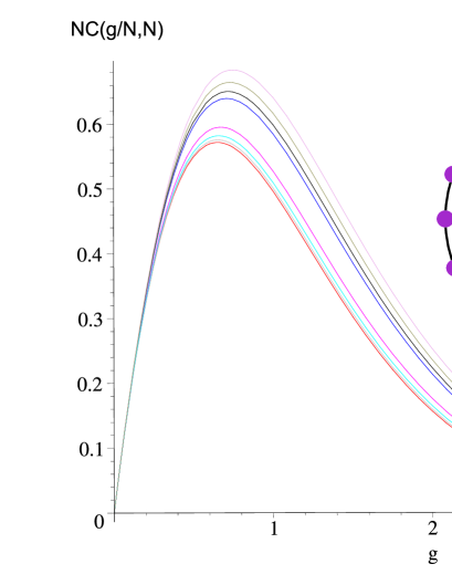
FIG. 1.: In the MPS ground state of (1), all the pairs of spins are equally entangled with each other. The curves show scaled concurrence for rings of size(from top to bottom) 6,7,8,9,10,20,30,40,and 50.

Let us briefly review the MPS formalism. On a ring of $N$ sites of $d-$level particles, a state is called a matrix product state if there exist matrices $A_{i},i=0,\cdots,d-1$ (of dimension $D$) such that

$$\psi_{i_{1},i_{2},\cdots,i_{N}}=\frac{1}{\sqrt{Z}}tr(A_{i_{1}}A_{i_{2}}\cdots A_{i_{N}}),$$ (5)

where $Z$ is a normalization constant given by $Z=tr(E^{N})$ in which $E:=\sum_{i=0}^{d-1}(A_{i}^{*}\otimes A_{i}).$ The state (5) is reflection symmetric if there exists a matrix $\Pi$ such that $A_{i}^{T}=\Pi A_{i}\Pi^{-1}$ (where $T$ means transpose) and time-reversal invariant if there exists a matrix $V$ such that $A_{i}^{*}=VA_{i}V^{-1}$. All the correlation functions can be calculated exactly. For example, for a local observable $O$, one finds

$$\langle\Psi|O(k)|\Psi\rangle=\frac{tr(E^{k-1}E_{O}E^{N-k})}{tr(E^{N})},$$ (6)

where $E_{O}:=\sum_{i,j=0}^{d-1}\langle i|O|j\rangle A_{i}^{*}\otimes A_{j}.$ In the thermodynamic limit ($N\rightarrow\infty$), only the eigenvector(s) corresponding to the eigenvalue $\lambda_{max}$ of $E$ with the largest absolute value matters and any level-crossing in this eigenvalue leads to a discontinuity in correlation functions.
Given a matrix product state, the reduced density matrix of $k$ adjacent sites is given by

$$\rho_{i_{1}\cdots i_{k},j_{1}\cdots j_{k}}=\frac{tr((A_{i_{1}}^{*}\cdots A_{i_{k}}^{*}\otimes A_{j_{1}}\cdots A_{j_{k}})E^{N-k})}{tr(E^{N})}.$$

This density matrix has at least $d^{k}-D^{2}$ zero eigenvalues. To see this, suppose that we can find complex numbers $c_{i_{1}\cdots i_{k}}$ such that

$$\sum_{j_{1},\cdots,j_{k}=0}^{d-1}c_{j_{1}\cdots j_{k}}A_{j_{1}}\cdots A_{j_{k}}=0.$$ (7)

This is a system of $D^{2}$ equations for $d^{k}$ unknowns which has at least $d^{k}-D^{2}$ independent solutions. Any such solution gives a null eigenvector of $\rho$. Thus for the density matrix of $k$ adjacent sites to have a null space, it is sufficient (but not necessary) that $d^{k}\ >\ D^{2}.$ Let the null space of the reduced density matrix be spanned by the orthogonal vectors $|e_{\alpha}\rangle,\alpha=1,\cdots,s$, then we can construct the local Hamiltonian acting on $k$ consecutive sites as

$$h:=\sum_{\alpha=1}^{s}J_{\alpha}|e_{\alpha}\rangle\langle e_{\alpha}|,$$

where $J_{\alpha}$ are positive constants. The total Hamiltonian on the chain will then be given by the positive operator $\ \ H=\sum_{l=1}^{N}h_{l,l+k},\$ where $h_{l,l+k}$ is the embedding of $h$ into sites $l$ to $l+k$ of the chain. The state $|\psi\rangle$ will then be a ground state of $H$. Equation ($d^{k}>D^{2}$) puts a stringent requirement on the dimensions of the matrices used in construction of a matrix product state. When dealing with spin $1/2$ with nearest-neighbor interactions, for which $d=2$ and $k=1$, it appears that the only admissible dimension for the matrices $A_{0}$ and $A_{1}$ is $D=1$, leading to a product state. However, it is crucial to note that the condition $d^{2}>D^{2}$ is only a sufficient and not a necessary condition for the density matrix $\rho$ to have a null space.
To proceed with our construction, we require that the state satisfy some natural symmetries, i.e. spin-flip symmetry which, in the language of matrix product formalism, means that there is a matrix $X$ such that

$$XA_{0}X^{-1}=\epsilon A_{1},\ \ \ XA_{1}X^{-1}=\epsilon A_{0},$$

where $\epsilon^{2}=1$. Working in the basis where $X=\sigma_{z}$, we find the general form of the matrices $A_{0}$ and $A_{1}$:

$$A_{0}=\left(\begin{array}[]{cc}a&b\\ c&d\end{array}\right)\hskip 28.45274ptA_{1}=\epsilon\left(\begin{array}[]{cc}a&-b\\ -c&d\end{array}\right).$$

Although these two matrices are not symmetric, the state constructed from them is symmetric under parity, since there is a matrix $\Pi=\left(\begin{array}[]{cc}b&0\\ 0&c\end{array}\right)$ with the property

$$\Pi A_{0}^{t}\Pi^{-1}=A_{0},\hskip 28.45274pt\Pi A_{1}^{t}\Pi^{-1}=A_{1}.$$

We now consider the matrix equation (7) which in the present case is

$$c_{00}A_{0}^{2}+c_{01}A_{0}A_{1}+c_{10}A_{1}A_{0}+c_{11}A_{1}^{2}=0.$$ (8)

This is a set of linear equations for the four coefficients $c_{ij}$, which can be written as a matrix equation $MC=0$, leading to a non-zero solution when

$$det(M)\equiv 16b^{2}c^{2}(a-d)^{2}(a+d)^{2}=0.$$

Thus we will find non-trivial models, for $a=d$ or $a=-d$. The models with $b=0$ or $c=0$ are not symmetric under parity, since in these cases the matrix $\Pi$ will not be invertible. We can always re-scale the matrices by a constant factor without affecting the matrix product state, so we set $a=1$ and use a subsequent gauge transformation $A_{i}\rightarrow SA_{i}S^{-1}$ with $S=\left(\begin{array}[]{cc}c&0\\ 0&1\end{array}\right)$, to set $c=1$. Therefore we are left with the following four classes of models defined by the matrices

$$A_{0}=\left(\begin{array}[]{cc}1&g\\ 1&\eta\end{array}\right)\hskip 28.45274ptA_{1}=\epsilon\left(\begin{array}[]{cc}1&-g\\ -1&\eta\end{array}\right),$$ (9)

where $g$ is a continuous parameter and $(\epsilon,\eta)=\pm(1,\pm 1)$. The four types of models are distinguished by the values of the pair $(\epsilon,\eta)$. The eigenvalues of the matrix $E=A_{0}\otimes A_{0}+A_{1}\otimes A_{1}$ are $2(\eta\pm g),\ \ 2(1\pm g)\ .$ The correlation functions can be derived from (6). Consider for definiteness, the case $\eta=1$. The magnetization per site is found from (6) to be

$$\langle\sigma_{y}\rangle=\langle\sigma_{z}\rangle=0,\hskip 28.45274pt\langle\sigma_{x}\rangle=\epsilon{u}\frac{1+u^{N-2}}{1+u^{N}},$$

where $u:=\frac{1-g}{1+g}$ and the correlation functions $G_{a}(1,r):=\langle\sigma_{a,1}\sigma_{a,r}\rangle$ are similarly found to be as follows:

$$G_{x}(1,r)=\frac{u^{2}+u^{N-2}}{1+u^{N}},$$ (10)

$$G_{y}(1,r)=\frac{u^{N-2}(u^{2}-1)}{1+u^{N}},\ \ G_{z}(1,r)=\frac{1-u^{2}}{1+u^{N}}.$$ (11)

These correlation functions satisfy the following relations:

$$G_{x}+G_{y}+G_{z}=1\ \ ,\ \ (1-G_{z})(1-G_{y})=\langle\sigma_{x}\rangle^{2}.$$ (12)

In the thermodynamic limit ($N\rightarrow\infty$), discontinuities develop in these correlation functions at $g=0$. For example, the magnetization per site will be

$$\langle\sigma_{x}\rangle=\epsilon\frac{1+|g|}{1-|g|},$$

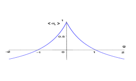
FIG. 2.: (Color Online)The magnetization in the $x$ direction as a function of $g$, ($\epsilon=1$).

and displayed in figure (2). Interestingly, the spins align themselves opposite to the magnetic field. To understand this, let us set for definiteness $\epsilon=\eta=1$ and consider the two-body Hamiltonian $H_{2}$, after subtracting the ferromagnetic term $-J{\sigma}\cdot{\sigma}$ for which any product state $|\phi\rangle|\phi\rangle$ is an eigenstate. For $|g|\gg 1$ the remaining Hamiltonian tends to $H_{2}\sim g^{2}(\frac{1}{2}\sigma_{1x}\sigma_{2x}+\sigma_{1x}+\sigma_{2x})$ , with the ground state $|x-\rangle|x-\rangle$ and for $|g|\ll 1$ it tends to $H_{2}\sim(\frac{1}{2}\sigma_{1x}\sigma_{2x}-\sigma_{1x}-\sigma_{2x})$, with the ground state $|x+\rangle|x+\rangle$. It is thus the combination of the anti-ferromagnetic interaction in the $x$ direction and the magnetic field which align the spins opposite to the magnetic field. Even when we tune the coupling $J$ so that there is no $xx$ coupling, (i.e. $J=(1+g^{2})/2$ ) this anti-alignment happens. To understand this, consider $g\approx 1$, where $H_{2}\approx-\sigma_{1z}\sigma_{2z}+B(\sigma_{1x}+\sigma_{2x})$ with $B$ very small. The ground state of this Hamiltonian is $|\psi\rangle\approx|\phi_{+}\rangle-B|\psi_{+}\rangle$, where $|\psi_{+}\rangle$ and $|\phi_{+}\rangle$ are Bell states. One then finds that $\langle\sigma_{1x}+\sigma_{2x}\rangle=-4B$, confirming figure (2).

In order to see how the Hamiltonian is constructed, we solve equations (8) which in view of (9) take the form

$$(1+g)(C_{00}+C_{11})+\epsilon(1-g)(C_{01}+C_{10}) = 0$$ (13)

$$(1+\eta)(C_{00}-C_{11})-\epsilon(1-\eta)(C_{01}-C_{10}) = 0.$$ (14)

It is easy to verify that the solution space is determined by the following two un-normalized vectors,

$$|e_{1}\rangle = (1+\eta)|\psi_{-}\rangle+(1-\eta)|\phi_{-}\rangle$$

$$|e_{2}\rangle = (1+g)|\psi_{+}\rangle-\epsilon(1-g)|\phi_{+}\rangle,$$

where $|\psi_{\pm}\rangle=\frac{1}{\sqrt{2}}(|0,1\rangle\pm|1,0\rangle)$ and $|\phi_{\pm}\rangle=\frac{1}{\sqrt{2}}(|0,0\rangle\pm|1,1\rangle)$ are Bell states. Under spin flip the above states transform as $|e_{1,2}\rangle\longrightarrow\mp|e_{1,2}\rangle$. The final local Hamiltonian will be given by $h=J|e_{1}\rangle\langle e_{1}|+|e_{2}\rangle\langle e_{2}|,$ where $J$ is a non-negative parameter and we have used the freedom for rescaling the couplings of the Hamiltonian to set one of the parameters equal to 1. In view of the symmetry property of the vectors under spin flip, this Hamiltonian will be symmetric under spin flip. Expressing the above operator in terms of Pauli operators and subtracting constant terms, we find the total Hamiltonian which is written in (1) and (3).
Note that the models with $\epsilon=\pm 1$ (sign of the magnetic field) are related by local $\pi$-rotations of spins around the $z$ axis where ($\sigma_{x,y}\rightarrow-\sigma_{x,y}$). Also, the models with $\eta=\pm$ are related to each other by simultaneous rotations $R_{x}(\frac{\pi}{2})\otimes R_{x}(\frac{-\pi}{2})$ of spins on adjacent sites, under which we have ($\sigma_{z,i}\sigma_{z,i+1}\rightleftharpoons-\sigma_{y,i}\sigma_{y,i+1})$. This is, of course, possible only when $N$ is even [13].

The explicit form of such a ground state can also be determined. For $\eta=1$, the matrices $A_{0}$ and $A_{1}$ commute. By a similarity transformation which does not change the state (5), both the matrices are made diagonal,

$$A_{0}=\left(\begin{array}[]{cc}1+\sqrt{g}&0\\ 0&1-\sqrt{g}\end{array}\right)\ ,A_{1}=\left(\begin{array}[]{cc}1-\sqrt{g}&0\\ 0&1+\sqrt{g}\end{array}\right)$$

and the MPS state (5) will be given by

$$|\Psi\rangle_{\eta=1}=\frac{1}{\sqrt{Z}}(|\phi_{+}\rangle^{\otimes N}+|\phi_{-}\rangle^{\otimes N}),$$ (15)

where

$$|\phi_{\pm}\rangle=(1\pm\sqrt{g})|0\rangle+(1\mp\sqrt{g})|1\rangle,$$

and $Z=2^{N+1}((1+g)^{N}+(1-g)^{N})$. These expressions are valid for all values of $g$, provided that we replace $\sqrt{g}\longrightarrow i\sqrt{-g}$ when we consider negative values of $g$. Note that $\langle\phi_{+}|\phi_{-}\rangle=2(1-g)$. One can indeed check that the separate product states are ground states of $H$, (i.e. the local Hamiltonian acting on two adjacent sites, when added by a suitable constant, annihilates $|\phi_{\pm}\rangle^{\otimes 2}$). However the advantage of the MPS state we have constructed $|\phi_{+}\rangle^{\otimes N}+|\phi_{-}\rangle^{\otimes N}$ or the other state $|\phi_{+}\rangle^{\otimes N}-|\phi_{-}\rangle^{\otimes N}$ is that they are invariant under spin-flip transformation $\sigma_{x}^{\otimes N}$. Thus even if the couplings of the Hamiltonian are not tuned as exactly as in (3), and are perturbed a little bit, first order perturbation theory guarantees that one of these entangled states and not the product states, will be the unique grounds state of $H$.

We now come to the entanglement properties of the state (15). At $g=1$ when $\langle\phi_{+}|\phi_{-}\rangle=0$, the state becomes a standard GHZ state, $\frac{1}{\sqrt{2}}(|0\cdots 0\rangle+|1\cdots 1\rangle)$. For other values of $g$, when $|\phi_{+}\rangle$ and $|\phi_{-}\rangle$ are no longer orthogonal, it can be named a generalized $GHZ$ state. Obviously such a state induces equal entanglement between any two spins regardless of their distance. To calculate this entanglement we determine the reduced two particle density matrix and use Wootters formula [11], with the result [12]:

$$C=\frac{4|g|}{|(1+g)^{N}+(1-g)^{N}|}|1-|g||^{N-2}.$$

Thus although the ring is not totally connected, the mutual entanglement of all pairs are equal and independent of their distances. Looking at the $N\gg 1$ limit, one can obtain the relation

$$NC(\frac{g}{N},N)\approx\frac{2|g|e^{-|g|}}{\cosh g}.$$ (16)

One can interpret the left hand side as the total mutual entanglement of a spin with all the other spins, and the above equation as a universal scaling relation for this total entanglement.

For the case $\eta=-1$, we use the transformation $U:=R_{x}(\frac{\pi}{2})\otimes R_{x}(\frac{-\pi}{2})$ on adjacent sites which transforms $H(\eta=1)$ to $H(\eta=-1)$ and act on (15) by $U^{\otimes\frac{N}{2}}$ to obtain the ground state as

$$|\Psi\rangle_{\eta=-1}=\frac{1}{\sqrt{Z}}(|\chi_{+}\rangle|\chi_{-}\rangle)^{\otimes\frac{N}{2}}+(|\chi_{-}\rangle|\chi_{+}\rangle)^{\otimes\frac{N}{2}},$$ (17)

where

$$|\chi_{\pm}\rangle=(1+\sqrt{g})|y,\pm\rangle\ \pm\ i(1-\sqrt{g})|y,\mp\rangle,$$

in which $|y,\pm\rangle$ denote the eigenstates of $\sigma_{y}$. An alternative way for deriving this ground state and indeed the reason for its simple structure, is to note that for $\eta=-1$, although the matrices $A_{0}$ and $A_{1}$ do not commute, the pairs of matrices corresponding to Bell states, defined by

$$\Phi_{mn}:=\frac{1}{\sqrt{2}}(A_{0}A_{m}+(-1)^{n}A_{1}A_{1+m}),\ \ m,n=0,1$$

commute with each other. The reader can verify that the states $|\chi\rangle_{\pm}|\chi_{\mp}\rangle$ are indeed linear combinations of the Bell states $\phi_{00}\equiv\phi_{+}$ , $\phi_{01}\equiv\psi_{-}$ and $\phi_{10}\equiv\psi_{+}$, making the state (17) a linear superposition of strings of various Bell states on adjacent sites.
In summary we have introduced a two-parameter family of spin 1/2 ${\rm xyz}$ Heisenberg chains, with nearest neighbor interactions in an external magnetic field, for which ground states and all correlation functions can be calculated exactly. These states have two very interesting properties: first, they undergo a discontinuous (quantum phase) transition as one of the parameters passes a critical point, which stimulates further exploration of MPS-quantum phase transition in a set of important exactly solvable models. Second, they have the property that all the pairs of spins are equally entangled with each other. This makes them good candidates for engineering long-range entanglement in experimentally realizable arrays of qubits or spin systems. This study can be extended in several directions, including generalization to open chains, finding the excitations, perturbing them to explore more models, and actual engineering of such chains for small number of qubits for information processing tasks. We thank David Gross, of Imperial college, London for a very stimulating email correspondence which led to substantial improvement of this paper and also A. Langari and M. R. Rahimitabar, for their valuable comments. Corresponding author, V. Karimipour, vahid@sharif.edu.

REFERENCES

- [1] V. E. Korepin and O. I. Patu, preprint, Cond-Mat/0701491.
- [2] I. Affleck, T. Kennedy, E.H. Lieb and H. Tasaki, Phys. Rev. Lett. 59, 799 (1987).
- [3] M. Fannes, B. Nachtergaele and R. F. Werner, Europhys. Lett. 10 633, (1989), A. Klumper, A. Schadschneider, J. Zittartz, J. Phys. A 24 L955 (1991); Z. Phys. B, 87, 281 (1992).
- [4] M. M. Wolf, G. Ortiz, F. Verstraete, J. I. Cirac, Phys. Rev. Lett.97, 110403 (2006); D. Peres Garcia, et al, quant-ph/0608197.
- [5] F. Verstraete, M.A. Martin-Delgado, J.I. Cirac, Phys. Rev. Lett. 92, 087201 (2004); F. Verstraete, M. Popp, J.I. Cirac, Phys. Rev. Lett. 92, 027901 (2004); F. Verstraete, J.I. Cirac, J.I. Latorre, E. Rico, M.M. Wolf, Phys.Rev.Lett. 94 (2005) 140601.
- [6] H. Fan, V. E. Korepin and V. Roychowdhury, Phys. Rev. Letts., 93, 227203 (2004); A. R. Its, B.-Q. Jin, and V. E. Korepin, Jour. Phys. A. Math. Gen. 38, 2975 (2005).
- [7] A. Osterloh, L. Amico, G. Falci and R. Fazio, Nature 416, 608 (2002); T. J. Osborne, and M. A. Nielsen, Phys. Rev. A 66, 032110 (2002); M. C. Arnesen, S. Bose, and V. Vedral, Phys. Rev. Lett. 87, 277901 (2001); M. Cozzini, Radu Ionicioiu, and Paulo Zanardi, Quantum fidelity and quantum phase transition in matrix product states, Cond-mat/0611727.
- [8] K. M. O’Connor and W. K. Wootters, Phys. Rev. A 63 (2001) 052302; M. Asoudeh, and V. Karimipour, Phys. Rev. A 70, 052307 (2004).
- [9] Here we are exlcuding the application of the MPS formalizm in stochastic systems, where ground state of non-hermitian matrices represent steady state of a stochastic process, B. Derrida, M.R. Evans, V. Hakim, V. Pasquier, J. Phys. A, 26, 1493 (1993), V. Karimipour, Phys. Rev. E59, 205 (1999).
- [10] S. Sachdev, Quantum Phase Transitions (Cambridge University Press, Cambridge, 1999).
- [11] W. K. Wootters, Phys. Rev. Letts. 80, 2245 (1998).
- [12] With conditions (12), the matrix has only two non-zero eigenvalues given by which gives
- [13] For and such an MPS does not exist, i.e. is identical to zero. One can prove this by induction using the facts that , and and are all proportional to identity.