Phase detection at the quantum limit with multi-photon Mach-Zehnder interferometry

Abstract

We study a Mach-Zehnder interferometer fed by a coherent state in one input port and vacuum in the other. We explore a Bayesian phase estimation strategy to demonstrate that it is possible to achieve the standard quantum limit independently from the true value of the phase shift and specific assumptions on the noise of the interferometer. We have been able to implement the protocol using parallel operation of two photon-number-resolving detectors and multiphoton coincidence logic electronics at the output ports of a weakly-illuminated Mach-Zehnder interferometer. This protocol is unbiased and saturates the Cramer-Rao phase uncertainty bound and, therefore, is an optimal phase estimation strategy.

The Mach-Zehnder (MZ) interferometer Mach ; Zehnder is a truly ubiquitous device that has been implemented using photons, electrons Ji_2003 , and atoms berman ; mm . Its applications range from micro- to macro-scales, including models of aerodynamics structures, near-field scanning microscopy zenhausern_1995 and the measurement of gravity accelerations peters_1999 . The central goal of interferometry is to estimate phases with the highest possible confidence Holland_1993 ; Sanders_1995 ; Pezze_2006 while taking into account sources of noise. Recent technological advances make it possible to reduce or compensate the classical noise to the level where a different and irreducible source of uncertainty becomes dominant: the quantum noise. Given a finite energy resource, quantum uncertainty principles and back reactions limit the ultimate precision of a phase measurement. In the standard configuration of the MZ interferometer, a coherent optical state with an average number of photons $\bar{n}=|\alpha|^{2}$ enters input port $a$ and the vacuum enters input port $b$, as illustrated in Figure (1). The goal is to estimate the value of the phase shift $\theta$ after measuring a certain number of photons $N_{c}$ and $N_{d}$ at output ports $c$ and $d$, which, in the experiment discussed in this Letter, is made possible by two number-resolving photodetectors.

The conventional phase inference protocol estimates the true value of the phase shift $\theta$ as Sculli ; Dowling_1998 ; Caves_1981 :

$$\Theta_{\text{est}}=\arccos\Big{(}\frac{M_{p}}{\bar{n}}\Big{)},$$ (1)

where $M_{p}=\sum_{k=1}^{p}(N_{c}^{(k)}-N_{d}^{(k)})/p$ is the photon number difference detected at the output ports, averaged over $p$ independent measurements. The phase uncertainty of estimator (1) is

$$\Delta\Theta=\frac{1}{\sqrt{p\,\bar{n}}\sin\theta},$$ (2)

which follows from a linear error propagation theory. Eq.(2) predicts an optimal working point at a phase shift $\theta=\pi/2$, where the average photon number difference varies most quickly with phase. As $\theta$ approaches 0 or $\pi$, the confidence of the measurement becomes very low and eventually vanishes.

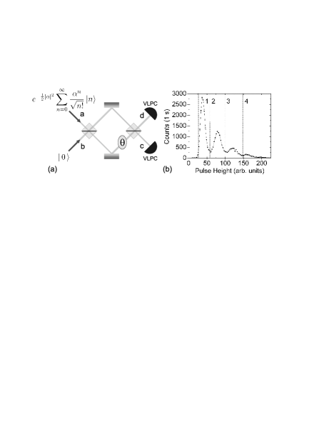
Figure 1: (a) Schematic of a Mach-Zehnder interferometer. A phase sensitive measurement is provided by the detection of the number of particles $N_{c}$ and $N_{d}$ at the two output ports. (b) Pulse height distribution for a visible light photon counter (VLPC) used in the experiment. The power incident on the detector is $144$ fW at a wavelength of 780 nm. The vertical lines show the decision thresholds Khoury_2006 .

As a consequence, this interferometric protocol does not allow the measurement of arbitrary phase shifts. This can be a serious drawback for applications like laser gyroscopes, the synchronization of clocks, or the alignment of reference frames. Furthermore, to estimate small phase shifts with the highest resolution, the interferometer has to be actively stabilized around $\pi/2$. This generally requires the addition of a feedback loop, which can be quite costly in terms of time and energy resources.

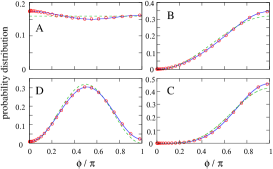
Figure 2: (color online). Phase distribution $P(\phi|N_{c},N_{d})$, for: A) $N_{c}=0$, $N_{d}=0$; B) $N_{c}=0$, $N_{d}=1$; C) $N_{c}=1$, $N_{d}=1$; D) $N_{c}=0$, $N_{d}=2$. The circles are the experimental data collected in the calibration part of the experiment, the dashed line is the ideal phase distribution Eq.(4). The solid line is a fit of the data according to Eq.(5).

It was first noticed by Yurke, McCall and Klauder (YMK) in Yurke_1986 that the estimator (1) does not take into account all the available information, and, in particular, the fluctuations in the total number of photons at the output ports. The possibility to improve Eq.(2) is confirmed by the analysis of the Cramer-Rao lower bound (CRLB) Cramer ; Rao , which provides, given an input state and choice of observables, the lowest uncertainty allowed by Quantum Mechanics. For a generic, unbiased, estimator, $\Delta\Theta_{CRLB}=1/\sqrt{pF(\theta)}$, where $F(\theta)$ is the Fisher information Fisher , which, in general, can depend on the true value of the phase shift $\theta$ and the number of independent measurements $p$. A direct calculation of the Fisher information for the coherent $\otimes$ vacuum input state, gives $F(\theta)=\bar{n}$. Therefore, the Cramer-Rao lower bound is

$$\Delta\Theta_{CRLB}=\frac{1}{\sqrt{p\,\bar{n}}},$$ (3)

which, in contrast with the result of Eq.(2), is independent of the true value of the phase shift. The only assumption here is that the observable measured at the output ports is the number of particles. It is well known (see for instance Helstrom ) that the Maximum Likelihood (ML) estimator, defined as the maximum, $\Theta_{ML}$, of the Likelihood function $P(N_{c},N_{d}|\phi)$ (see below), saturates the CRLB, but only asymptotically in the number of measurements $p$. In the current literature there have been alternative suggestions to obtain an unbiased estimator and a phase independent sensitivity with a Mach-Zehnder interferometer Yurke_1986 ; Hradil_1996 ; Berry_2000 ; Sanders_1995 ; NFM_1991 . They will be specifically addressed at the end of this Letter.

Here we develop a protocol based on a Bayesian analysis of the measurement results Helstrom ; Holland_1993 ; Hradil_1996 ; Pezze_2006 . The goal is to determine $P(\phi|\,N_{c},N_{d})$, the probability that the phase equals $\phi$ given the measured $N_{c}$ and $N_{d}$. Bayes’ theorem provides this: $P(\phi|N_{c},N_{d})=P(N_{c},N_{d}|\phi)~{}P(\phi)/P(N_{c},N_{d})$, where $P(N_{c},N_{d}|\phi)$ is the probability to detect $N_{c}$ and $N_{d}$ when the phase is $\phi$ nota2 , $P(\phi)$ quantifies our prior knowledge about the true value of the phase shift, and $P(N_{c},N_{d})$ is fixed by normalization. Assuming no prior knowledge of the phase shift, $P(\phi)=1/\pi$. In the ideal case, the Bayesian phase probability distribution can be calculated analytically for any value of $N_{c}$ and $N_{d}$,

$$P(\phi|N_{c},N_{d})=\mathcal{C}\Big{(}\cos\frac{\phi}{2}\Big{)}^{2N_{c}}\Big{(}\sin\frac{\phi}{2}\Big{)}^{2N_{d}},$$ (4)

where $\mathcal{C}=\frac{\Gamma(1/2+N_{c})\Gamma(1/2+N_{d})}{\Gamma(1+N_{c}+Nd)}$ is a normalization constant. In practice, one must measure $P(N_{c},N_{d}|\phi)$ and, from this, determine $P(\phi|N_{c},N_{d})$. This distribution provides both an estimate on the phase and the uncertainty in this estimate.

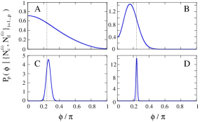
Figure 3: (color online). Phase probability distribution Eq.(6), obtained after $p$ independent experimental measurements $\{N_{c}^{(i)},N_{d}^{(i)}\}_{i=1..p}$: A) $p=1$, B) $p=10$, C) $p=100$, D) $p=1000$. The true value of the phase shift is $\theta/\pi=0.24$, shown by the vertical dashed line.

There are several advantages to using a Bayesian protocol. Notably, it can be applied to any number $p$ of independent measurements, it does not require statistical convergence or averaging, and it provides uncertainty estimates tailored to the specific measurement results. For instance, with a single measurement, $p=1$, it predicts an uncertainty that scales as $\Delta\Theta\approx\frac{1}{\sqrt{N_{c}+N_{d}}}$. Since Eq.(4) does not depend on $\bar{n}$, the estimation is insensitive to fluctuations of the input laser intensity. Most importantly, its uncertainty, in the limit $p>>1$, is $\Delta\Theta=\frac{1}{\sqrt{p\,\bar{n}}}$ which coincides with the CRLB.

To implement the proposed protocol we have realized a polarization Mach-Zehnder interferometer with photon-number-resolving coincidence detection. In a recent paper we reported on the analysis of a coherent state using a single photon-number-resolving detector Khoury_2006 . We have extended this experimental capability to two simultaneously operating visible light photon counters (VLPCs) Turner , cryogenic photodetectors that provide a current pulse of approximately 40,000 electrons per detected photon. The VLPCs were maintained at 8 K in a helium flow cryostat, and their photocurrent was amplified by low-noise, room temperature amplifiers. We measured a detection efficiency of 35% and a dark count rate of $3\times 10^{5}$ for each detector under our operating conditions. Custom electronics processed the amplified VLPC current pulses to perform gated, fast coincidence detection. We were thus able to determine, for each pulse, how many photons were detected at both ports $c$ and $d$. A Ti:sapphire pulsed laser, attenuated such that $\bar{n}=1.08$ photons, provided the input state. Since a coherent state maintains its form under linear loss Sculli , the presence of loss after the interferometer is completely equivalent to a lossless interferometer fed by a weaker input state. We use $\bar{n}$ to signify the average number of photons in the detected state per pulse, after all losses. We were limited by the amplifiers to measuring up to four photons per pulse Fig. 1(b), but at $\bar{n}=1.08$ the probability of detecting five or more photons is negligible. The phase shift $\theta$ was changed by tilting a birefringent crystal inside the interferometer.

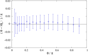
Figure 4: (color online). Difference between the mean value of the phase estimator, $\langle\Theta_{\text{est}}\rangle$, obtained after 150 replica of $p=1000$ independent measurements and the true value of the phase shift $\theta$. The vertical bars are the mean square fluctuations $\sigma_{est}^{2}=\langle(\Theta_{est}-\langle\Theta_{\text{est}}\rangle)^{2}\rangle$. The result $\sigma_{est}\gg(\theta-\Theta_{est})$ proves that our protocol provides an unbiased experimental phase estimation.

The first part of the experiment consists of the calibration of the interferometer. At different, known, values of the phase shift, we measured $N_{c}$ and $N_{d}$ for each of $200,000$ laser pulses. This procedure allows us to determine experimentally both $P(N_{c},N_{d}|\phi)$ and $P(\phi|N_{c},N_{d})$. In Fig.(2) we compare the ideal and the experimental phase distributions. The agreement is quite good, and the discrepancies can be attributed to imperfect photon-number discrimination by the detectors. To fit the data in Fig.(2), we introduce the probability $P(N_{c},N_{d}|N_{c}^{\prime},N_{d}^{\prime})$ to measure $N_{c}$ and $N_{d}$ when $N_{c}^{\prime}$ and $N_{d}^{\prime}$ photons were really present. Taking this into account, the experimental phase probability distribution is

$$P_{\text{fit}}(\phi|N_{c},N_{d})=\sum_{N_{c}^{\prime},N_{d}^{\prime}}P(\phi|N_{c}^{\prime},N_{d}^{\prime})P(N_{c}^{\prime},N_{d}^{\prime}|N_{c},N_{d}),$$ (5)

where $P(\phi|N_{c}^{\prime},N_{d}^{\prime})$ are the ideal probabilities Eq.(4). The weights $P(N_{c}^{\prime},N_{d}^{\prime}|N_{c},N_{d})$ can be retrieved from a fit of the experimental calibration distributions $P(\phi|N_{c},N_{d})$, see Fig.(2). The quantity $P(N_{c},N_{d}|N_{c},N_{d})$, equal to one in the ideal case, is 0.54 in Fig.(2A) (corresponding to the worst case among all distributions), 0.67 in (2B) and (2C), and 0.87 in (2D).

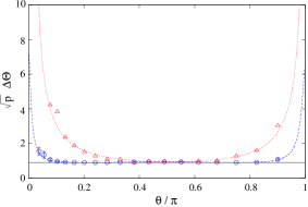
Figure 5: (color online). Phase sensitivity as a function of the true value of the phase shift. Circles are obtained from Bayesian distributions Eq.(6), with $p=1000$. The error bars give the fluctuations of $\sqrt{p}\,\Delta\Theta$ obtained with 150 independent replica of the experiment. The solid black line is the theoretical prediction Eq.(3). The dashed blue line is the CRLB calculated with the experimental distributions. Triangles are the uncertainty obtained with a generalization of the estimator Eq.(1) taking into account the experimental imperfections, while the dotted red line is the phase sensitivity predicted by Eq.(2).

After the calibration, we can proceed with the Bayesian phase estimation experiment. For a certain value of the phase shift, we input one laser pulse and detect the number of photons $N_{c}$ and $N_{d}$. We repeat this procedure $p$ times obtaining a sequence of independent results $\{N_{c}^{(i)},N_{d}^{(i)}\}_{i=1\ldots p}$. The $p$ photon-number measurements comprise a single phase estimation. The overall phase probability is given by the product of the distributions associated with each experimental result:

$$P\big{(}\phi|\{N_{c}^{(i)},N_{d}^{(i)}\}_{i=1\ldots p}\big{)}\propto\prod_{i=1}^{p}P_{\text{fit}}\big{(}\phi|N_{c}^{(i)},N_{d}^{(i)}\big{)}.$$ (6)

The phase estimator $\Theta_{\text{est}}$ is given by the mean value of the distribution, $\Theta_{\text{est}}=\int_{0}^{\pi}\mathrm{d}\phi\,\phi\,P\big{(}\phi|\{N_{1}^{(i)},N_{2}^{(i)}\}_{i=1\ldots p}\big{)}$, and the phase uncertainty $\Delta\Theta$ is the $68.27\%$ confidence interval around $\Theta_{\text{est}}$. An example of $P\big{(}\phi|\{N_{c}^{(i)},N_{d}^{(i)}\}_{i=1\ldots p}\big{)}$ is given in Fig.(3), for $\theta/\pi=0.24$ and for different values of $p$. Since the average number of photons of the coherent input state is small, for $p\sim 1$ the phase uncertainty is of the order of the prior knowledge, $\Delta\Theta\simeq\pi$. As $p$ increases, the probability distribution becomes Gaussian and the sensitivity scales as $\Delta\Theta\propto 1/\sqrt{p}$, in agreement with the central limit theorem.

In Fig.(4), we show the difference between the mean value of the phase estimator $\langle\Theta_{\text{est}}\rangle$, obtained from 150 phase estimations, each with $p=1000$, and the true value of the phase shift. The bars are the mean square fluctuation. The important result is that our protocol provides an experimentally unbiased phase estimation over the entire phase interval.

The main result of this Letter is presented in Fig.(5). We show the phase sensitivity for different values of the phase shift $\theta$, calculated from the distribution Eq.(6) with $p=1000$ photon-number measurements. The circles are the mean value of $\Delta\Theta$, and the bars give the corresponding mean square fluctuation, obtained from 150 independent phase measurements. The dashed blue line is the CRLB calculated with the experimental probability distributions, $\Delta\theta_{\mathrm{fit}}=1/\sqrt{pF_{\mathrm{fit}}(\theta)}$, where $F_{\mathrm{fit}}(\theta)=\sum_{N_{1},N_{2}}\frac{1}{P_{\mathrm{fit}}(N_{1},N_{2}|\theta)}(\frac{\partial P_{\mathrm{fit}}(N_{1},N_{2}|\theta)}{\partial\theta})^{2}$ nota3 . For $0.1\lesssim\theta/\pi\lesssim 0.9$, it follows the theoretical prediction (solid black line), Eq.(3), where $\bar{n}=1.08$ has been independently calculated from the collected data. Around $\theta=0,\pi$, where the photons have higher probability to exit through the same output port, $\Delta\theta_{\mathrm{fit}}$ increases as a consequence of the decreased sensitivity of our detectors to higher photon number states. Even though the phase sensitivity of our apparatus becomes worse near $\theta=0,\pi$, it never diverges. Triangles show the phase uncertainty obtained with Eq.(1), but taking into account the experimental noise. The estimator is obtained by inverting the equation $M_{p}=\bar{n}\cos(a+\theta)+b$ nota1 . This strategy provides an unbiased estimation with a sensitivity close to the one predicted by Eq.(2) (dotted red line). The reason for the superior performance of the Bayesian protocol can be understood by noticing that, in Eq.(2), the phase estimate is retrieved only from the measurement of the photon number difference, which, simply does not exploit all of the available information.

In Yurke_1986 YMK first proposed a generalization of the estimator Eq.(1) to take into account the whole information in the output measurements. Their estimator, $\Theta_{\text{YMK}}=\arccos[(N_{c}-N_{d})/(N_{c}+N_{d})]$, gives a phase independent sensitivity, $\Delta\Theta=1/\sqrt{N_{c}+N_{d}}$. Notice that $\Theta_{\text{YMK}}$ coincides with the Maximum Likelihood estimator in the ideal, noiseless, MZ interferometer. However, it is not obvious how to generalize $\Theta_{\text{YMK}}$ for real interferometry, where classical noise is present and the YMK estimator is different from $\Theta_{ML}$. In general, because of correlations between $N_{c}-N_{d}$ and $N_{c}+N_{d}$, this estimator becomes strongly biased in the presence of noise as we have verified using our experimental data Pezze . Moreover, the YMK estimator cannot be extended when both input ports of the interferometer are illuminated. Conversely, the Bayesian analysis holds for general inputs and, in particular, it predicts a phase-independent sensitivity when squeezed vacuum is injected in the unused port of the MZ Pezze , which reaches a sub shot-noise sensitivity Caves_1981 . It should be noted that detection losses again become important when attempting to use nonclassical light to overcome the shot-noise limit Eq.(3).

In Hradil_1996 , Hradil et al. used a Bayesian approach for a Michelson-Morley neutron interferometer (single output detection) and discussed theoretically the MZ. Their analysis was based on specific assumptions about the interferometric classical noise which are not satisfied in the case discussed in this Letter. Different approaches with adaptive measurements Berry_2000 and positive operator value measurements Sanders_1995 have been also suggested. While these strategies might be important for interferometry at the Heisenberg limit, they are not necessary in our case.

In conclusion, we have presented a Bayesian phase estimation protocol for a MZ interferometer fed by a single coherent state. The protocol is unbiased and provides a phase sensitivity that saturates the ultimate Cramer-Rao uncertainty bound imposed by quantum fluctuations. We have been able to implement the protocol with two photon-number-resolving detectors at the output ports of a weakly-illuminated interferometer. Yet, the method can be generalized to the case of high intensity laser interferometry and photodiode detectors. In this case, the limit Eq.(3) becomes harder to achieve because of larger electronic noise and lower photon number resolution, however it should still be possible to demonstrate a phase independent sensitivity. Our results are of importance to quantum inference theory and show that the MZ interferometer does not require phase-locking in order to reach an optimal sensitivity.

Acknowledgment. This work has been partially supported by the US DoE and NSF Grant No. 0304678.

References

- (1) L. Mach, Zeitschr. f. Instrkde. 12, 89 (1892).
- (2) L. Zehnder, Zeitschr. f. Instrkde. 11, 275 (1891).
- (3) Y. Ji, et al., Nature 422, 415 (2003).
- (4) Atom Interferometry. P.R. Berman edt., Academic Press, New York, 1997.
- (5) Y. Wang et al., Phys. Rev. Lett. 94, 090405 (2005).
- (6) F. Zenhausern, Y. Martin & H.K. Wickramasinghe, Science 269, 1083 (1995).
- (7) A. Peters, K.Y. Chung & S. Chu, Nature 400, 849 (1999).
- (8) M.J. Holland & K. Burnett. Phys. Rev. Lett. 71, 1355 (1993).
- (9) L. Pezzé & A. Smerzi, Phys. Rev. A 73, 011801(R) (2006).
- (10) B.C. Sanders & G.J. Milburn, Phys. Rev. Lett. 75, 2944 (1995).
- (11) M.O. Scully & M.S. Zubairy, Quantum Optics, Cambridge University Press 1997.
- (12) J.P. Dowling, Phys. Rev. A 57, 4736 (1998).
- (13) C.M. Caves, Phys. Rev. D 23, 1693 (1981).
- (14) B. Yurke, S.L. McCall & J.R. Klauder, Phys. Rev. A 33, 4033 (1986).
- (15) H. Cramer. Mathematical methods of statistics, Princeton, Princeton university press, 1946.
- (16) C.R. Rao, Bull. Calcutta Math. Soc. 37, 81 (1945).
- (17) R.A. Fisher, Proc. Camb. Phi. Soc. 22, 700 (1925).
- (18) C.W. Helstrom, Quantum Detection and Estimation Theory Academic Press, New York, 1976.
- (19) Z. Hradil, et al., Phys. Rev. Lett. 76, 4295-4298 (1996).
- (20) D.W. Berry & H.M. Wiseman, Phys. Rev. Lett. 85, 5098 (2000).
- (21) J.W. Noh, A. Fougeres & L. Mandel, Phys. Rev. Lett. 67, 1426 (1991); J. Rehacek, et al., Phys. Rev. A 60, 473 (1991).
- (22) The Quantum Mechanical probability to detect and particles at the output port and , respectively, is given by , where , with bosonic annihilation operators. For the configuration studied in this Letter .
- (23) G. Khoury, et al., Phys. Rev. Lett. 96, 203601 (2006).
- (24) G.B. Turner, et al., Proceedings of the Workshop on Scintillating Fiber Detectors, Notre Dame University, edited by R. Ruchti (World Scientific, Singapore, 1994).
- (25) A fit of the calibration data gives , with and .
- (26) The distributions are obtained from Eq.(5) with the Bayes theorem.
- (27) Manuscript in preparation.