Effect of finite detection efficiency on the observation of the dipole-dipole interaction of a few Rydberg atoms

Abstract

We have developed a simple analytical model describing multiatom signals that are measured in experiments on dipole-dipole interaction at resonant collisions of a few Rydberg atoms. It has been shown that finite efficiency of the selective field-ionization detector leads to the mixing up of the spectra of resonant collisions registered for various numbers of Rydberg atoms. The formulas which help to estimate an appropriate mean Rydberg atom number for a given detection efficiency are presented. We have found that a measurement of the relation between the amplitudes of collisional resonances observed in the one- and two-atom signals provides a straightforward determination of the absolute detection efficiency and mean Rydberg atom number. We also performed a testing experiment on resonant collisions in a small excitation volume of a sodium atomic beam. The resonances observed for 1-4 detected Rydberg atoms have been analyzed and compared with theory.

I INTRODUCTION

Experimental and theoretical studies of long-range interactions of highly excited Rydberg atoms are important for the development of quantum information processing with neutral atoms [1]. Strong dipole-dipole (DD) or van der Waals interactions between Rydberg atoms allow for entanglement of neutral atoms and implementation of quantum logic gates [2-7]. Practical realization of the proposed schemes for two-qubit phase gates [2, 4-6] and dipole blockade [3, 7] demands the precise measurements of the number of Rydberg atoms, since two or single atoms must be unambiguously detected in these schemes.

High detection efficiency of Rydberg atoms is thus a key issue for implementing the quantum information processing. The most sensitive detection of Rydberg atoms is achieved with the selective field ionization (SFI) technique that in addition allows for measurements of the population distribution [8]. A typical timing diagram of the SFI detection is shown in Fig.1(a). A ramp of the electric field is applied after each laser excitation pulse at delay $t_{0}$ that defines the time of free Rydberg-Rydberg interaction. Rydberg atoms ionize with almost 100% probability as soon as the electric field reaches a critical value $E_{cr}\sim n^{-4}$, where n is the principal quantum number. The resulting electrons or ions are detected either by a channeltron or by a microchannel plate (MCP) detector.

For experiments with a few Rydberg atoms the channeltron is preferred, since the amplitudes of the channeltron’s output pulses are peaked near well-resolved equidistant maxima corresponding to the different numbers of detected particles. As an example, in Fig.1(b) a histogram of the amplified output pulses of the channeltron VEU-6 (GRAN, Russia) used in our experiments is presented. It exhibits the distinct maxima corresponding to the 1$-$5 electrons from the sodium Rydberg atoms detected by SFI after the excitation by pulsed lasers.

Detection efficiency of channeltrons may reach 90% [9]. However, several factors may significantly reduce the overall SFI detection probability. These are metallic meshes of finite transparency $T=(50-90)\%$ used to form a homogeneous electric field and to extract charged particles to the channeltron’s input window [see Fig.4(a) for our experimental arrangement], dependence of detection efficiency on the energy and type of charged particles (electrons or ions), contamination of the channeltron’s working surface after exposure to the atmosphere, etc. These factors can negatively affect the signals and spectra measured in experiments on long-range interactions of a few Rydberg atoms.

The main purpose of this paper is to analyze theoretically and experimentally the effect of reduced (and actually unknown) detection efficiency on the observed spectra of resonant collisions of a few Rydberg atoms. Such collisions are mediated by DD interaction and lie at the heart of the dipole-blockade effect and other related schemes of quantum information processing. They were investigated in numerous experiments [10-24], but detection statistics at resonance collisions of a few Rydberg atoms was not studied yet (although recently a sub-Poissonian statistics of the MCP signals at the laser excitation of about 30 Rydberg atoms was studied both experimentally [25] and theoretically [26, 27]). We have also implemented a new method to determine the absolute values of the detection efficiency and mean number of Rydberg atoms excited per laser pulse. These issues are important for the further development of quantum information processing with Rydberg atoms.

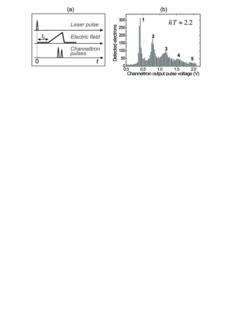
Figure 1: (a) A typical timing diagram of experiments with selective field ionization (SFI) of Rydberg atoms. (b) The histogram of the amplified output pulses of a channeltron used in our experiments. The observed peaks correspond to 1$-$5 electrons from the sodium Rydberg atoms detected with SFI after the excitation by pulsed lasers. The mean number of atoms detected per laser pulse $\bar{n}T$ is about 2.2.

II Laser excitation and detection statistics for Rydberg atoms

For N₀ ground-state atoms in the laser excitation volume and probability of excitation for one atom $0\leq p\leq 1$ the mean number of Rydberg atoms excited per laser pulse is

$$\bar{n}=p\,N_{0}$$ (1)

The statistics of the number of Rydberg atoms excited by each laser shot depends on p. In the case of weak excitation (for example, by pulsed broadband laser radiation that is often used in experiments) with $p\ll 1$ a Poisson distribution for the probability $P_{N}^{weak}$ to detect N Rydberg atoms after a single laser shot is applicable:

$$P_{N}^{weak}=\frac{{\left({\bar{n}}\right)^{N}}}{{N!}}\,\mathrm{e}^{-\,\bar{n}}$$ (2)

In the case of strong excitation (for example, for coherent excitation of Rydberg atoms by narrow-band lasers [28, 29]) a normal distribution must be used

$$P_{N}^{strong}=p^{N}\left({1-p}\right)^{N_{0}-N}\frac{{N_{0}!}}{{N!\left({N_{0}-N}\right)!}}$$ (3)

It is valid for any p and N₀ and provides general solutions for the measured signals from Rydberg atoms, although analytical formulas obtained with Eq.(3) may be rather complicated.

In the further analysis we will ignore a possible effect of the dipole blockade on the above distributions which was discussed in Refs. [25, 26], i.e., Rydberg-Rydberg interactions during exciting laser pulses will be neglected. This is the case for appropriately short laser pulses. In this approximation, the above probability distributions would be observed with an ideal SFI detector of Rydberg atoms. However, for a real detector with the detection efficiency T it can be shown that these distributions change to

$$\bar{P}_{N}^{weak}=\frac{{\left({\bar{n}T}\right)^{N}}}{{N!}}\,\mathrm{e}^{-\,\bar{n}T}\qquad\qquad\qquad\qquad\qquad$$ (4)

$$\bar{P}_{N}^{strong}=\left({p\,T}\right)^{N}\left({1-p\,T}\right)^{N_{0}-N}\frac{{N_{0}!}}{{N!\left({N_{0}-N}\right)!}}$$ (5)

The mean number of Rydberg atoms detected per laser shot thus reduces to $\bar{n}T$. This value can be measured experimentally. For example, the amplitudes of the peaks in the histogram of Fig.1(b) are proportional to $\bar{P}_{N}^{weak}$. Therefore, the relation between the integrated single-atom and two-atom peaks is $\bar{P}_{2}^{weak}/\bar{P}_{1}^{weak}=\bar{n}T/2$, and our measurement gave $\bar{n}T\approx 2.2$. The relations between the other integrated multiatom peaks are also well described by Eq.(4) at $\bar{n}T\approx 2.2$, confirming that the Poisson statistics is valid for the channeltron signals.

Thus, a pure interaction of, e.g., two Rydberg atoms cannot be observed with nonideal SFI detectors, since measured two-atom signals would have a contribution from the larger numbers of Rydberg atoms. This is also true for possible observations of the dipole blockade, which should appear as laser excitation of only one Rydberg atom out of many interacting atoms due to the interaction-induced changes in the spectra of collective excitations [3]. Our aim is to analyze what detection efficiency is tolerable for experiments of such kind.

As the number of Rydberg atoms excited in each laser shot is unknown and fluctuates around $\bar{n}$, a post-selection technique should be used in order to measure the signals for a definite number N of Rydberg atoms detected per laser pulse. In this technique the signals are first accumulated over many laser pulses. Then they are sorted by the number of atoms (up to 5 atoms in our experiments) according to the measured in advance histogram of the channeltron’s output pulses [Fig.1(b)]. After this procedure the signals are separately determined for various N. This technique has been demonstrated in our previous experiment on microwave spectroscopy of multiatom excitations [5].

III Resonant collisions

Dipole-dipole interaction of Rydberg atoms appears most prominently in resonant collisions (also called F$\ddot{\mathrm{o}}$rster resonances), which have huge cross-sections [8]. Population transfer between Rydberg states induced by such processes is a sensitive probe of DD interaction in atomic beams [10-13] and cold atom clouds [14-24].

In the present work we have analyzed the Rydberg atom statistics and effect of finite detection efficiency on the observed spectra of resonant collisions of a few sodium Rydberg atoms, both theoretically and experimentally. A particular collisional resonance under study was the population transfer in the binary collisions:

$$\mathrm{Na}(37\mathrm{S})+\mathrm{Na}(37\mathrm{S})\to\mathrm{Na}(36\mathrm{P})+\mathrm{Na}(37\mathrm{P})$$ (6)

where Na(nL) stands for a sodium Rydberg atom in highly-excited nL state. Processes of this kind were observed in many alkali-metal atoms and for various resonances. In the case of sodium, the energy resonance arises when the $n$S state lies midway between the $n$P and $(n-1)$P states. The resonance of Eq.(6) is tuned by the Stark effect in the electric field 6.3-7.2 V/cm [Fig.2(a)], depending on the fine-structure components of P-states. It appears as narrow peaks in the dependence of population of the 37P state on the electric field after initial excitation of atoms to the 37S state. An example of collisional resonances observed in our experiment with a velocity-selected atomic beam is shown in Fig.2(b) for the case of one Rydberg atom detected with the post-selection technique. We note that the 37P sodium atoms are separately detected by SFI, while the 37S and 36P atoms have almost identical critical electric fields for SFI and cannot be individually detected.

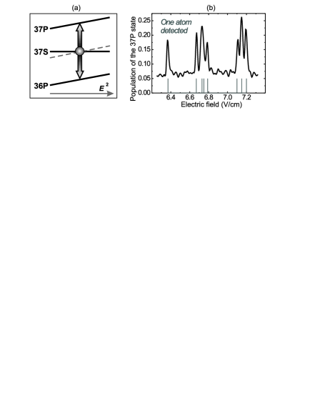
Figure 2: (a) Sodium energy levels for the resonant collisions Na(37S)+Na(37S)$\to$Na(36P)+Na(37P) tuned by the electric field E. (b) An example of the experimental spectrum of collisional resonances in a velocity-selected atomic beam for the case of one sodium Rydberg atom detected. The vertical lines indicate the calculated positions of resonances for various fine-structure components of P states.

Nonresonant background processes that can also populate the 37P state should be taken into account for the full signal analysis. These are transitions induced by the ambient 300 K blackbody radiation (BBR) [8] and by nonresonant collisions. They give a constant background signal, which is independent of the number of Rydberg atoms and electric field [Fig.2(b)].

The signals of resonant collisions can be independently measured for various numbers N of detected Rydberg atoms by accumulating the statistics over many laser pulses and by their post-selecting. The normalized N-atom signals measured in our experiments are

$$S_{N}=\frac{{n_{N}\left({37\mathrm{P}}\right)}}{{n_{N}\left({37\mathrm{S}}\right)+n_{N}\left({36\mathrm{P}}\right)+n_{N}\left({37\mathrm{P}}\right)}}$$ (7)

where $n_{N}\left({nL}\right)$ is the total number of nL Rydberg atoms detected by SFI during the accumulation time for the particular case of N detected Rydberg atoms. An example of the experimental signal $S_{1}$ is shown in Fig.2(b).

For an ideal SFI detector Eq.(7) simply gives the population $\rho_{N}$ (normalized per 1) of the 37P state in a Rydberg atom after having interacted with (N$-$1) surrounding Rydberg atoms. The approximate formulas for $\rho_{N}$ will be obtained in Sec.V. For the nonideal detector, various $\rho_{N}$ contribute to $S_{N}$ in a degree that depends on $\bar{n}T$, as it will be shown below.

IV Multiatom signals at finite detection efficiency

Expressions describing $n_{N}\left({nL}\right)$ can be explicitly written for any N:

$$\left\{{{\begin{array}[]{*{20}l}{n_{N}\left({37\mathrm{P}}\right)=}\\ {\quad Z\sum\limits_{i=N}^{N_{0}}{NP_{i}\,\rho_{i}\,T^{N}\left({1-T}\right)^{i-N}\displaystyle\frac{{i!}}{{N!\left({i-N}\right)!}}}}\\ {}\\ {n_{N}\left({37\mathrm{S}}\right)+n_{N}\left({36\mathrm{P}}\right)=}\\ {\quad Z\sum\limits_{i=N}^{N_{0}}{NP_{i}\,\left({1-\rho_{i}}\right)\,T^{N}\left({1-T}\right)^{i-N}\displaystyle\frac{{i!}}{{N!\left({i-N}\right)!}}}}\\ \end{array}}}\right.$$ (8)

where $Z\gg 1$ is the number of exciting laser pulses during the accumulation time and $P_{i}$ is the probability distribution given either by Eq.(2) or Eq.(3). Each term in the above sums represents the contribution from i actually excited Rydberg atoms, and it takes into account its statistical weight and finite detection probability. Each $\rho_{i}$ should be viewed as a collision resonance contour, which would be observed for the interaction of i Rydberg atoms. The radiation dumping of Rydberg states is neglected here, i.e., the interaction time is assumed to be much shorter than their effective lifetimes of $\simeq$30 $\mu$s (37S state) and $\simeq$70 $\mu$s (36P and 37P states) at the 300 K ambient temperature.

Taking into account that

$$n_{N}\left({37\mathrm{P}}\right)+n_{N}\left({37\mathrm{S}}\right)+n_{N}\left({36\mathrm{P}}\right)=ZN\bar{P}_{N}$$ (9)

where $\bar{P}_{N}$ is the probability distribution given either by Eq.(4) or Eq.(5), the measured, post-selected and averaged over $Z$ laser pulses signals of resonant collisions are

$$S_{N}^{weak}=\mathrm{e}^{-\bar{n}\left({1-T}\right)}\sum\limits_{i=N}^{\infty}{\rho_{i}\frac{{\left[{\bar{n}\left({1-T}\right)}\right]^{i-N}}}{{\left({i-N}\right)!}}}\qquad$$ (10)

$$S_{N}^{strong}=\displaystyle\frac{{\left({N_{0}-N}\right)!}}{{\left({N_{0}-\bar{n}T}\right)^{N_{0}-N}}}\times\qquad\qquad\qquad\qquad$$

$$\times\sum\limits_{i=N}^{N_{0}}{\rho_{i}\displaystyle\frac{{\left[{\bar{n}\left({1-T}\right)}\right]^{i-N}\left({N_{0}-\bar{n}}\right)^{N_{0}-i}}}{{\left({N_{0}-i}\right)!\left({i-N}\right)!}}}$$ (11)

For an ideal detector $(T=1)$ the expected identity $S_{N}=\rho_{N}$ is obtained with both distributions, since only the $i=N$ term in the sum is nonzero.

We should note that $\rho_{1}$ cannot have a collision resonance feature, since this is a single-atom spectrum. The population transfer in $\rho_{1}$ may appear only due to the mentioned background processes from BBR and nonresonant collisions. At the same time, the other spectra (i.e., $\rho_{N>1}$) must have a constant non-resonant part identical to $\rho_{1}$ (as it is independent of the electric field) and a resonant part $\rho_{N}^{res}$ from Rydberg-Rydberg interactions:

$$\rho_{N>1}=\rho_{1}+\rho_{N}^{res}$$ (12)

The substitution of Eq.(12) into Eq.(10), Eq.(IV), and their reduction yield

$$S_{N}^{weak}=\rho_{1}+\,\mathrm{e}^{-\bar{n}\left({1-T}\right)}\sum\limits_{i=N}^{\infty}{\rho_{i}^{res}\displaystyle\frac{{\left[{\bar{n}\left({1-T}\right)}\right]^{i-N}}}{{\left({i-N}\right)!}}}$$ (13)

$$S_{N}^{strong}=\rho_{1}+\displaystyle\frac{{\left({N_{0}-N}\right)!}}{{\left({N_{0}-\bar{n}T}\right)^{N_{0}-N}}}\times\qquad\qquad\qquad$$

$$\times\sum\limits_{i=N}^{N_{0}}{\rho^{res}_{i}\displaystyle\frac{{\left[{\bar{n}\left({1-T}\right)}\right]^{i-N}\left({N_{0}-\bar{n}}\right)^{N_{0}-i}}}{{\left({N_{0}-i}\right)!\left({i-N}\right)!}}}$$ (14)

In order to compare the observed amplitudes of collisional resonances, the nonresonant background $\rho_{1}$ should be subtracted from these signals.

Equations (13) and (IV) help to estimate the detection error and the contributions from the higher numbers of actually excited Rydberg atoms. For example, the signal $S_{1}$ is important to study the dipole blockade, where excitation of only one Rydberg atom by any laser excitation pulse is expected. With an ideal detector ($T=1$) the collisional resonance in $S_{1}$ must be absent. With nonideal detector ($T<1$) the resonance must also be absent at the full blockade, but it may appear at the partial blockade, when two or more atoms are excited. Therefore, the amplitude of the resonance in $S_{1}$ can be a measure of the blockade efficiency. Following Refs. [25, 26], the full blockade must also result in a complete disappearance of the peaks with $N\geq 2$ in the histogram of Fig.1(b).

The signal $S_{2}$ is important to study two-atom interactions and to implement two-qubit quantum phase gate. We see from Eq.(13) that pure two-atom interactions in $S_{2}$ can be observed only when $\bar{n}\left({1-T}\right)\ll 1$, i.e., either $\bar{n}$ should be sufficiently small or $T$ must be close to 1. More conclusions will be drawn after evaluating the dependences of $\rho_{N}^{res}$ on N in the next section.

V Evaluation of the multiatom spectra of resonant collisions

Accurate calculation of $\rho_{N}^{res}$ is a challenging problem. It requires to account for many-body interactions [30, 31], orientation of atom dipoles [18, 21, 32], time evolution of dipoles and populations [23, 27, 31], spatial distribution of Rydberg atoms [18, 21, 33], coherent and pumping effects at the laser excitation [20, 28, 29], etc.

On the other hand, as we are interested mainly in obtaining a scaling dependence of $\rho_{N}^{res}$ on $N$, this problem can be significantly simplified by using the perturbation theory in a limit of weak DD interaction. For this purpose we will introduce an average energy of DD interaction between any pair of Rydberg atoms in the atomic ensemble. This corresponds to the spatial and orientational averaging of laser excitation and of Rydberg dipoles over the ensemble. Such approximation is reasonable, since we study the signals averaged over many laser excitation and detection events in a disordered atomic ensemble.

The Hamiltonian of the ensemble is

$$\hat{H}=\sum\limits_{k=1}^{N_{0}}{\hat{H}_{k}+\sum\limits_{n\neq m}{\hat{V}_{nm}}}$$ (15)

where $\hat{H}_{k}$ is the unperturbed Hamiltonian of the kth atom, and $\hat{V}_{nm}$ is the operator of binary DD interaction of the arbitrary nth and mth atoms:

$$\hat{V}_{nm}=\frac{{1}}{{4\pi\varepsilon_{0}}}\left[{\frac{{\hat{\mathbf{d}}_{n}\hat{\mathbf{d}}_{m}}}{{R_{nm}^{3}}}-\frac{{3\,\,\left({\hat{\mathbf{d}}_{n}\mathbf{R}_{nm}}\right)\,\left({\hat{\mathbf{d}}_{m}\mathbf{R}_{nm}}\right)}}{{R_{nm}^{5}}}}\right]$$ (16)

Here $\hat{\mathbf{d}}_{n}$ and $\hat{\mathbf{d}}_{m}$ are dipole moment operators of the nth and mth atoms, $\mathbf{R}_{nm}$ is a vector connecting these two atoms, and $\varepsilon_{0}$ is the dielectric constant. The sum over $V_{nm}$ in Eq.(15) accounts for all possible binary interactions and contains $N(N-1)$ terms.

Our aim is to evaluate $\rho_{N}^{res}$ for a given number N of actually excited Rydberg atoms. In order to do that, we must decompose the wave function of the atom ensemble to a set of the collective states corresponding to the different numbers of Rydberg atoms and then proceed with the calculations for certain N. Analytical calculations are possible only for a weak DD interaction, i.e., when the 37P state is weakly populated. In the resonance approximation the two-atom transition amplitudes $a_{nm}$ for the process of Eq.(6) are found from

$$a_{nm}\left({t_{0}}\right)\approx-i\;\int\limits_{0}^{t_{0}}{\Omega_{nm}\left({t}\right)\,\mathrm{e}^{-i\Delta t}dt}$$ (17)

Here $t_{0}$ is the interaction time and $\Delta=\left({2\mathrm{E}_{37\mathrm{S}}-\mathrm{E}_{36\mathrm{P}}-\mathrm{E}_{37\mathrm{P}}}\right)/\hbar$ is the detuning from the resonance, which is determined by the Stark-tuned energies E_nL of the Rydberg states shown in Fig.2(a). The value $\hbar\Omega_{nm}(t)$ is the energy of the resonant DD interaction between nth and mth atoms.

After calculating the time dependences of a_nm, the desired spectra $\rho_{N}^{res}$ can be found from

$$\rho_{N}^{res}=\frac{{1}}{{N}}\sum\limits_{n\neq m}{\left|{a_{nm}}\right|^{2}}$$ (18)

Each value $\left|{a_{nm}}\right|^{2}$ is the probability of two atoms $n$ and $m$ out of N Rydberg atoms to simultaneously leave the initial 37S state and undergo the transitions to the final 36P and 37P states. The factor 1/N appears because in this final collective state the population of the 37P state per atom is $1/N$. Other collective states with two or more 37P atoms are not populated at weak DD interaction. Therefore, the main problem is the calculation of $a_{nm}$ and $\rho_{N}^{res}$ for particular experimental conditions. We will consider a frozen Rydberg gas and an atomic beam, which differ in the time dependence of the interaction energy.

V.1 Frozen Rydberg gas

In a frozen Rydberg gas [14, 15] the atoms are almost immobile during the free interaction time [$t_{0}$ in Fig.1(a)] of a few microseconds [23]. In this case $\Omega_{nm}$ are constants, and $a_{nm}$ are readily calculated from Eq.(17). Then Eq.(18) yields

$$\rho_{N}^{res}\left({t_{0}}\right)\approx\frac{{\sin^{2\,}\left({\,t_{0}\Delta/2}\right)}}{{N\;\left({\Delta/2}\right)^{2}}}\sum\limits_{n\neq m}{\left|{\Omega_{nm}}\right|}^{2}$$ (19)

The full width at half maximum (FWHM) of this resonance is $\approx 1/t_{0}$ and it is independent of N at the weak DD interaction. For the analysis of its amplitude we may note that the sum in Eq.(19) has $N(N-1)$ terms and therefore can be represented as

$$\sum\limits_{n\neq m}{\left|{\Omega_{nm}}\right|^{2}\equiv N\left({N-1}\right)\,\Omega^{2}}$$ (20)

where $\hbar\Omega$ is the mean-square energy of resonant DD interaction between any pair of atoms in the ensemble. The averaging must be made over all possible positions of 2 Rydberg atoms among $(N_{0}-2)$ ground-state atoms in the laser excitation volume. We note that Eq.(20) has a general form that gives a correct result even at $N=1$, when DD interaction must be absent.

The value of $\Omega^{2}$ depends on the atom density and geometry of the excitation volume [21]. Its accurate analytical or numerical calculation must be a subject of a special study and lies beyond the scope of this paper. We shall only estimate it in the following qualitative manner.

Let us consider the DD interaction between two arbitrary Rydberg atoms in the laser excitation volume containing $N_{0}\gg 1$ ground-state atoms. A peculiarity of this problem is that after the laser pulse any atom can be found in a Rydberg state. The number density $n_{0}$ of ground-state atoms defines the average spacing $R_{0}\approx\left({4\pi n_{0}/3}\right)^{-1/3}$ between two neighboring atoms. The energy of DD interaction of two Rydberg atoms spaced by $R_{0}$ is estimated from Eq.(16) as

$$\hbar\Omega_{0}\sim\frac{\left\langle{36\mathrm{P}\left|{\hat{\mathbf{\mathrm{d}}}}\right|37\mathrm{S}}\right\rangle\left\langle{37\mathrm{P}\left|{\hat{\mathbf{\mathrm{d}}}}\right|37\mathrm{S}}\right\rangle}{{4\pi\varepsilon_{0}R_{0}^{3}}}$$ (21)

Our aim is to express $\Omega^{2}$ through $\Omega_{0}$ and $N_{0}$. In the averaging procedure for $\Omega^{2}$ we will use the below qualitative argumentation that seems to be valid for disordered atom ensembles at $N_{0}\gg N$. Let the excitation volume has a spherical shape of radius $R\gg R_{0}$, so that the volume is $\mathrm{V}=4\pi R^{3}/3$. We have to find a mean-square energy of DD interaction of an atom, situated deeply in this volume, with the surrounding $(N_{0}-1)\approx N_{0}$ atoms. The mean atom number in the volume of radius $R_{0}$ is $4\pi R_{0}^{3}n_{0}/3=1$. This implies that on the average there are no other atoms at the distances $r<R_{0}$ from this central atom. Therefore, one should only account for the interactions of this atom with other atoms situated at $r\geq R_{0}$. The mean number of atoms at the distances lying in the interval from $r$ to $r+dr$ is $\left({n_{0}4\pi r^{2}dr}\right)$. Hence, the statistical weight of this spherical layer is $\left({n_{0}4\pi r^{2}dr/N_{0}}\right)$. Then the averaging is done with the integral

$$\Omega^{2}=\frac{{n_{0}}}{{N_{0}}}\int\limits_{R_{0}}^{R}{\frac{{\Omega_{0}^{2}R_{0}^{6}}}{{r^{6}}}\;4\pi r^{2}dr\approx\frac{{\Omega_{0}^{2}}}{{N_{0}}}}\;$$ (22)

The relations $N_{0}=n_{0}\mathrm{V}$ and $R\gg R_{0}$ have been applied here. The physical meaning of Eq.(26) is that the main contribution to $\Omega^{2}$ comes from the nearest-neighbor atom at $r\approx R_{0}$, which can be found in a Rydberg state with the $1/N_{0}$ probability. Other atoms on the average are situated at larger distances and their contribution has been estimated to be small. Although Eq.(26) gives only a rough estimate for the mean-square energy of DD interaction of two arbitrary Rydberg atoms in large disordered atom ensembles, it can be used in the approximate analytical calculations instead of more precise but complicated numerical simulations that must account for the actual geometry of the excitation volume.

Finally, we find that for the weak DD interaction the amplitude of the resonance scales as

$$\;\rho_{N}^{res}\left({t_{0},\;\Delta=0}\right)\sim(N-1)\;\frac{{\Omega_{0}^{2}}}{{N_{0}}}\;t_{0}^{2}$$ (23)

V.2 Atomic beam

Atoms in thermal atomic beams have a wide velocity spread (on the order of $v_{0}=\sqrt{2k_{\mathrm{B}}\mathrm{T}/M}\approx 680$ m/s at the $\mathrm{T}=650$ K temperature for Na, where $k_{\mathrm{B}}$ is the Boltzmann constant and M is the atom mass). Therefore, the energy of DD interaction of a pair of Rydberg atoms is most likely a rapidly varying function of time [10-13]:

$$\Omega_{nm}\left({t}\right)\sim\Omega_{0}\frac{{R_{0}^{3}}}{{\left[{v_{nm}^{2}\left({t-t_{nm}}\right)^{2}+b_{nm}^{2}}\right]^{3/2}}}$$ (24)

where $v_{nm}$ is the relative velocity of the two atoms, $b_{nm}$ is the impact parameter of collision, and $t_{nm}$ is the time moment when the interaction energy reaches its maximum. In the case of atomic beam both energy and time of interaction depend on the initial distance between the two Rydberg atoms.

At $v_{nm}\gg\left({b_{nm}/t_{0}}\right)$ each pair of Rydberg atoms interacts momentarily and only one time. The effective collision time obtained from Eq.(24) is $\tau_{nm}\approx 2b_{nm}/v_{nm}$. By analogy with Eq.(23), the estimated amplitude of the resonance for N Rydberg atoms at the weak DD interaction is

$$\;\rho_{N}^{res}\left({t_{0},\;\Delta=0}\right)\sim(N-1)\;\Omega^{2}_{beam}\tau^{2}$$ (25)

where $\tau$ is the mean collision time and $\hbar\Omega_{beam}$ is the mean-square interaction energy for any of the two atoms in the atomic beam. We may expect that the main contribution to the transition amplitude is also from the nearest-neighbor atoms. Then the collision time is $\tau\sim 2R_{0}/v_{0}$ and the width of the resonance is $\Gamma\sim 1/\tau$.

The value of $\Omega^{2}_{beam}$ differs from $\Omega^{2}$ in Eq.(22). Due to the relative motion of the atoms in the beam, each atom effectively interacts with the larger amount of atoms, than in the frozen gas. The approximate formula $\Omega_{beam}^{2}\sim\Omega_{0}^{2}/N_{0}^{2/3}$ has been obtained from averaging of Eq.(24) over the impact parameter instead of the interatomic distance in Eq.(22). A more accurate calculation of the resonance line shape for the atomic beam must be a subject of a special study. We only note that averaging over the velocity distribution may result in the cusp-shaped resonances (pointed at the top) due to the longer interaction time of atoms with low collision velocities [13].

V.3 Multiatom signals at weak DD interaction

Multiatom signals of Eq.(13) and Eq.(IV) can be further reduced using Eq.(23) or Eq.(25). The explicit N dependences of these equations allow us to represent any $\rho_{N}^{res}$ through the two-atom spectrum $\rho_{2}^{res}$ as

$$\rho_{N}^{res}=\left({N-1}\right)\,\rho_{2}^{res}$$ (26)

The substitution of Eq.(26) into Eq.(13) and Eq.(IV) gives after the sum reduction:

$$S_{N}^{weak}=\rho_{1}+\rho_{2}^{\mathrm{res}}\left[{N-1+\;\bar{n}\left({1-T}\right)}\right]$$ (27)

$$S_{N}^{strong}=\rho_{1}+\rho_{2}^{\mathrm{\mathrm{res}}}\left[{N-1+\;\bar{n}\left({1-T}\right)\frac{{1-\bar{n}/N_{0}}}{{1-\bar{n}T/N_{0}}}}\right]$$ (28)

It is seen that Eq.(27) can be obtained from Eq.(28) at $N_{0}\gg\mathrm{max}\left({1,\;\bar{n}T}\right)$. This is a criterion for the validity of the Poisson distribution, which means that the number of all atoms in the excitation volume must be much larger than 1 or than the number of detected Rydberg atoms.

The further analysis of signals will be performed with Eq.(27), which is applicable to most of the experimental conditions. For the correctness of measurements, the resonances in $S_{1}$ must be small compared to those in $S_{N>1}$. This is the case if $\bar{n}\ll 1/\left({1-T}\right)$, i.e., if the mean Rydberg atom number is limited to some maximum allowed value. This value is large if only $T$ is close to 1.

At $N>1$ the criterion of correct measurements changes to $\bar{n}\ll\left({N-1}\right)/\left({1-T}\right)$. In this case $S_{N}\approx\rho_{1}+\rho_{N}^{res}$, so that pure interaction of $N$ Rydberg atoms can be studied even with poor detectors, provided $\bar{n}$ is sufficiently low. For example, for $N=2$ and $T=0.1$ we must use $\bar{n}\ll 1$. In this case the necessary accumulation time is rather long, since the mean number of atoms detected per laser pulse is small ($\bar{n}T\ll 0.1$). For a good detector with $T=0.9$ we estimate $\bar{n}\ll 10$ and the accumulation time is two orders of magnitude shorter. From this point of view, the tolerable detection efficiency is estimated as $T\geq 0.5$, while the appropriate mean number of Rydberg atoms is $\bar{n}<1$.

Other interesting observations can be made for the relationships between various multiatom signals. In particular, the signals $S_{1}$ and $S_{2}$ are of major importance for the observations of the two-atom interactions and dipole blockade effect. For the Poisson distribution the ratio of their resonant parts is

$$\alpha=\frac{{S_{1}-\rho_{1}}}{{S_{2}-\rho_{1}}}=\frac{{\bar{n}\left({1-T}\right)\;}}{{1+\,\bar{n}\left({1-T}\right)}}$$ (29)

We can consider various limits of this relation. It is zero at $T=1$ since in this case there is no resonance in $S_{1}$. If $\bar{n}\left({1-T}\right)\ll 1$, it is close to $\bar{n}\left({1-T}\right)$. In the intermediate case $\bar{n}\left({1-T}\right)\sim 1$ the resonance in $S_{1}$ is about two times smaller than in $S_{2}$. However, at $\bar{n}\left({1-T}\right)\gg 1$ it approaches 1 and the resonances in $S_{1}$ and $S_{2}$ become of identical amplitudes and shapes, so that it would be impossible to investigate, e.g., pure two-atom interactions.

We have noticed that a measurement of $\alpha$ provides a straightforward determination of $\bar{n}\left({1-T}\right)$ without any knowledge about $\rho_{2}^{res}$:

$$\bar{n}\left({1-T}\right)=\frac{{\alpha}}{{1-\alpha}}$$ (30)

On the other hand, the mean number of Rydberg atoms detected per laser excitation pulse is $\beta=\bar{n}T$ and it can also be measured in experiments, e.g., from the histograms in Fig.1(b). Therefore, the two above measurements provide an unambiguous determination of the unknown experimental parameters $\bar{n}$ and $T$:

$$\left\{{{\begin{array}[]{*{20}l}{\bar{n}=\displaystyle\frac{{\alpha}}{{1-\alpha}}+\beta}\\ \\ {T=\beta/\bar{n}}\\ \end{array}}}\right.$$ (31)

These formulas are advantageous as they are independent of the specific experimental conditions (atom density, laser intensity, excitation volume, dipole moments, etc.), which are hard to measure in order to find $\bar{n}$ and $T$ with conventional methods. In fact, Eq.(31) provides a new method of the absolute $\bar{n}$ and $T$ measurements. The calculated dependences of T and $\bar{n}$ on the measured parameters $\alpha$ and $\beta$ are show in Fig.3.

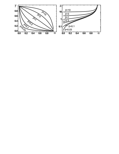
Figure 3: Calculated dependences of detection efficiency T and mean Rydberg atom number $\bar{n}$ on the parameters $\alpha=\left({S_{1}^{weak}-\rho_{1}}\right)/\left({S_{2}^{weak}-\rho_{1}}\right)$ and $\beta=\bar{n}T$, which can be measured in experiments.

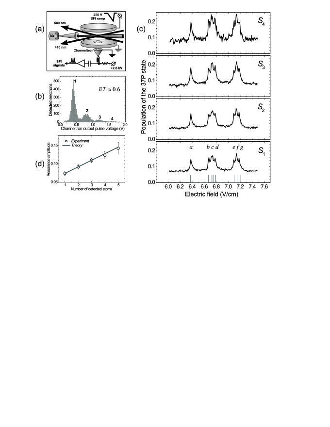
Figure 4: (a) An arrangement of the experiment on resonant collisions in Na atomic beam. (b) The histogram of the amplified output pulses of the channeltron measured at the mean number of atoms detected per laser pulse $\bar{n}T\approx 0.6$. (c) The experimental spectrum of collisional resonances observed in the Na atomic beam for 1-4 detected Rydberg atoms. The vertical lines indicate the calculated positions of resonances for various fine-structure components of P states. (d) The comparison between experiment and theory for the dependence of the amplitude of resonance a on the number of detected Rydberg atoms.

VI Experiment with a sodium atomic beam

The above theoretical analysis of the Rydberg atom statistics at the SFI detection of resonant collisions needs an experimental confirmation, since no experiments were made earlier for a few Rydberg atoms. We therefore have performed the first testing experiment with a sodium atomic beam, where post-selected signals of resonant collisions were studied for a few detected Rydberg atoms.

VI.1 Experimental setup

An experimental setup was the same as we used in our recent experiments on collisional and BBR ionization of sodium Rydberg atoms [34]. The Na effusive atomic beam with the 650 K temperature ($v_{0}\approx 680$ m/s) was formed in a vacuum chamber with the 5$\times$10^-7 Torr background pressure. The beam was passed between the two stainless-steel plates separated by 10 mm [Fig.4(a)]. A ramp of the pulsed voltage was applied to the upper plate for the SFI detection of Rydberg atoms. The lower plate had a 10-mm-diameter hole covered by a mesh with 70% geometrical transparency. The electrons that have appeared in the SFI were passed through this mesh to an input window of a channeltron. A weak dc electric field was added to the upper plate for the Stark tuning of resonant collisions.

The 37S_1/2 state was excited via the two-step scheme $3\mathrm{S}_{1/2}\to 3\mathrm{P}_{3/2}\to 37\mathrm{S}_{1/2}$. The first step at 589 nm was driven by either pulsed (5 kHz) or cw Rhodamine 6G dye-laser. The broadband pulsed radiation ($\simeq$20 GHz linewidth) could excite the atoms of all velocities, while the narrowband cw radiation ($\leq$10 MHz linewidth) provided a velocity selection at the cycling hyperfine transition 3S_1/2(F=2)$\to$3P_3/2(F^′=3). The second step at 410 nm was driven by the second harmonic of a pulsed titanium-sapphire laser having 5 kHz repetition rate, 50 ns pulses, and 10 GHz linewidth.

In order to work with a few strongly interacting Rydberg atoms, we had to localize a small excitation volume. We attained this using a crossed-beam geometry shown in Fig.4(a). The two exciting laser beams were focused and intersected at the right angles inside of the atomic beam. Both laser beams were set at the 45^∘ angles with respect to the atomic beam. In this way we formed the excitation volume of about 50 $\mu$m size that provided the mean spacing of a few microns between Rydberg atoms. The laser powers were adjusted to detect a few Rydberg atoms per laser pulse on the average.

The timing diagram of signals was identical to that of Fig.1(a) with the free DD interaction time $t_{0}=3$ $\mu$s. The channeltron output pulses from the 37P and (37S+36P) states were detected using two independent gates. The channeltron provided the atom-number resolution according to the measured histogram of Fig.4(b). Although the neighboring multiatom signals in the histograms are overlapping to some extent, the estimated fidelity of the correct N determination is $>$90$\%$ for the single-atom signal and $>$80$\%$ for the two-atom signal. The signals were automatically post-selected and sorted out according to the number of detected Rydberg atoms.

VI.2 Experimental results

The experiments on resonant collisions were performed at the volume density $n_{0}\approx 8\times 10^{10}$ cm^-3 of ground-state atoms. This value corresponds to the average spacing between neighboring atoms $R_{0}\approx 1.44\;\mu m$ and to the atom number $N_{0}\approx 10^{4}$ in the $\mathrm{V}\approx 50\times 50\times 50\;\mu$m³ excitation volume. At this density the collision resonances were reliably observed in the $S_{1}$ signal with both pulsed and cw lasers at the first excitation step. The narrow resonances obtained with cw laser were presented in Fig.2(b). Unfortunately, the use of cw laser significantly reduced the number of atoms excited to the intermediate 3P_3/2 state due to the velocity selection and partial optical pumping to the 3S_1/2(F=1) ground state, so that detection of resonances in the $S_{2}-S_{4}$ signals required too long accumulation time. Therefore, the further experiments were performed with the pulsed laser in order to provide an appropriate signal-to-noise ratio in the multiatom signals, at the cost of somewhat broader resonances.

The multiatom spectra of resonant collisions $S_{1}-S_{4}$ observed with the pulsed 589 nm laser are presented in Fig.4(c). The spectrum for $S_{5}$ is not shown, since it had significant noise due to low probability of the detection of 5 atoms [see the histogram in Fig.4(b)]. The seven peaks $a-g$ in Fig.4(c) are due to various transitions to the fine-structure components of P states (actually, nine peaks must appear, but peaks $c$ and $f$ have two unresolved components). The positions of the resonances well coincide with the values obtained from the numerically calculated Stark map of the relevant Rydberg states [the vertical lines in Fig.4(c)]. In agreement with Ref. [13], the resonances tend to have a cusp shape, since the pointed tops of the two unresolved resonances in peak $c$ are well seen.

We will consider in more detail the resonance $36\mathrm{P}_{J=3/2,\,\left|{M_{J}}\right|=1/2}\leftrightarrow 37\mathrm{S}\leftrightarrow 37\mathrm{P}_{J=3/2,\,\left|{M_{J}}\right|=1/2}$ that corresponds to the well-resolved single peak a at $6.37$ V/cm. Its FWHM is $(35\pm 3)$ mV/cm. This width can be converted to the effective frequency width using the polarizabilities measured in our earlier microwave experiments [35]. The FWHM of resonance $a$ is $(53\pm 5)$ MHz. This experimental value well agrees with the roughly estimated width $1/(2\pi\tau)\sim v_{0}/(4\pi R_{0})\approx 40$ MHz.

As predicted by the theory, the amplitudes of the resonances in Fig.4(c) grow with the increase of the number of detected Rydberg atoms, although we expected this effect to be more pronounced. In order to compare the observed amplitude of resonance $a$ with theory, the radial parts of the dipole moments of the 37S$-$36P and 37S$-$37P transitions have been numerically calculated and found to be 1372 and 1439 a.u., correspondingly. The angular parts of both dipole moments are $\sqrt{2}/3$. From Eq.(21) and Eq.(22) we have obtained $\Omega_{0}/\left({2\,\pi}\right)\sim 150$ MHz and $\Omega/\left({2\,\pi}\right)\sim 1.5$ MHz. Then Eq.(25) yields the theoretical value $\rho_{2}^{res}\left({\Delta=0}\right)\sim 0.03$.

Further, at the pulsed laser excitation from the histogram of Fig.4(b) we have measured that the integral of the two-atom peak (taken over 0.6$-$1 V) is nearly 3.3 times smaller than the integral of the single-atom peak (taken over 0.2$-$0.6 V). Their ratio can be found from Eq.(4) as $\bar{P}_{2}^{weak}/\bar{P}_{1}^{weak}=\bar{n}T/2$, hence $\beta=\bar{n}T\approx 0.6$ in our experiment with the pulsed laser. The parameter $\alpha$ of Eq.(29) was determined from the observed relation $\left({S_{1}-\rho_{1}}\right)/\left({S_{2}-\rho_{1}}\right)\approx 0.075/0.095\approx 0.8$ between the single- and two-atom amplitudes of peak a in Fig.4(c). Finally, Eq.(31) yields the unknown experimental parameters $\bar{n}\approx(4.7\pm 0.5)$ and $T\approx(13\pm 1.5)\,\%$.

This relatively low detection efficiency was unexpected, since we specially installed a newly made channeltron and expected T to be close to the geometrical transparency of the detector mesh (70%). Our attempts to improve the SFI detection system (acceleration of electrons prior to detection, detection of ions instead of electrons, cleaning of the channeltron’s surface, etc.) did not noticeably increase the efficiency.

This observation contrasts with the recent paper [36], where simultaneous detection of ions and electrons, delivered from photoionization of Rb atoms, by two opposite channeltrons allowed to observe the 50% detection efficiency for ions. A dependence of the detection efficiency on the channeltron’s voltage has been additionally investigated in this work. It exhibited a strongly nonlinear behavior, with zero efficiency at 2.4 kV and 50% efficiency at 2.9 kV. Unfortunately, in our experiment we applied the 2.6 kV voltage specified by the manufacturer and did not vary it in a broad range. This seems to be the most likely reason for the lower detection efficiency in our case. This surmise will be tested in a forthcoming experiment with cold Rb Rydberg atoms. Another way to improve the detection efficiency could be the usage of the SFI detection system based on a set of resistively coupled parallel cylindrical plates, which provides a homogeneous electric field without a mesh [37].

Nevertheless, we have demonstrated that the above measurements provide a tool to determine unknown T, which may degrade during the course of any experiments and therefore should be periodically checked out. We may recommend our method to be applied in those experiments with Rydberg atoms where the absolute detection efficiency is crucial.

Finally, with the above experimental values for $\bar{n}$, $T$, and amplitude $S_{1}-\rho_{1}\approx 0.075$ of peak a, using Eq.(27) we have determined the experimental value $\rho_{2}^{res}\left({\Delta=0}\right)\approx(0.02\pm 0.004)$. It satisfactory agrees with the theoretical value 0.03, taking into account the approximations adopted in our theoretical model. Furthermore, we can compare the values for the amplitudes of observed resonances to those calculated with Eq.(27) at $\rho_{2}^{res}\left({\Delta=0}\right)=0.02$. These are shown in Fig.4(d), where we also added an experimental point for $S_{5}$ extracted from its noisy spectrum. The experimental and theoretical dependences coincide well for all N, showing a linear dependence and confirming the validity of Eq.(27). A comparison between experiment and theory for the other peaks in Fig.4(c) has also demonstrated a satisfactory quantitative agreement.

VII Conclusions

The developed theoretical model describes multiatom signals that are measured in the experiments on long-range interactions of a few Rydberg atoms. Although several simplifying approximations were used to obtain the analytical formulas, their validity has been partly confirmed by the satisfactory agreement with the first experimental data obtained for the resonant collisions of a few Rydberg atoms in the atomic beam. The main result is that finite detection efficiency of the selective field-ionization detector leads to the mixing up of the spectra of the resonant collisions associated with various numbers of actually excited atoms. In particular, the collisional resonance features may appear even in the single-atom signal if the detection efficiency is low. This may misinterpret the possible observations of the full dipole blockade or coherent two-atom collisions, which are required for quantum logic gates. The obtained formulas are helpful in estimating the appropriate mean number of Rydberg atoms excited per laser pulse at a given detection efficiency.

We have also shown that a measurement of the relation between the amplitudes of resonances observed in the single- and two-atom signals provides a straightforward determination of the absolute detection efficiency and mean Rydberg atom number. This new method is advantageous as it is independent of the specific experimental conditions (atom density, laser intensity, excitation volume, dipole moments, etc.).

The further experimental efforts should be focused on cold Rydberg atoms. This would help to test our model at the longer interaction times, which are of interest to quantum information processing. Microwave spectroscopy of resonant collisions [38, 39] can be additionally applied as a sensitive probe and control tool.

- (1) P. S. Jessen, D. L. Haycock, G. Klose, G. A. Smith, I. H. Deutsch, and G. K. Brennen, Quantum Information and Computation 1, 20 (2001).
- (2) D. Jaksch, J. I. Cirac, P. Zoller, S. L. Rolston, R. Cote, and M. D. Lukin, Phys. Rev. Lett. 85, 2208 (2000).
- (3) M. D. Lukin, M. Fleischhauer, R. Cote, L. M. Duan, D. Jaksch, J. I. Cirac, and P. Zoller, Phys. Rev. Lett. 87, 037901 (2001).
- (4) I. E. Protsenko, G. Reymond, N. Schlosser, and P. Grangier, Phys. Rev. A 65, 052301 (2002).
- (5) I. I. Ryabtsev, D. B. Tretyakov, and I. I. Beterov, J. Phys. B 38, S421 (2005).
- (6) M. Saffman and T. G. Walker, Phys. Rev. A 72, 022347 (2005).
- (7) M. Saffman and T. G. Walker, Phys. Rev. A 72, 042302 (2005).
- (8) Rydberg States of Atoms and Molecules, ed. by R. F. Stebbings and F. B. Dunning (Cambridge University Press, Cambridge, 1983); T. F. Gallagher, Rydberg Atoms (Cambridge University Press, Cambridge, 1994).
- (9) Burle Electro-Optics Inc., http://www.burle.com/cgi- bin/byteserver.pl/pdf/ChannelBook.pdf
- (10) K. A. Safinya, J. F. Delpech, F. Gounand, W. Sandner, and T. F. Gallagher, Phys. Rev. Lett. 47, 405 (1981).
- (11) T. F. Gallagher, K. A. Safinya, F. Gounand, J. F. Delpech, W. Sandner, and R. Kachru, Phys. Rev. A 25, 1905 (1982).
- (12) R. C. Stoneman, M. D. Adams, and T. F. Gallagher, Phys. Rev. Lett. 58, 1324 (1987).
- (13) J. R. Veale, W. Anderson, M. Gatzke, M. Renn, and T. F. Gallagher, Phys. Rev. A 54, 1430 (1996).
- (14) W. R. Anderson, J. R. Veale, and T. F. Gallagher, Phys. Rev. Lett. 80, 249 (1998).
- (15) I. Mourachko, D. Comparat, F. de Tomasi, A. Fioretti, P. Nosbaum, V. M. Akulin, and P. Pillet, Phys. Rev. Lett. 80, 253 (1998).
- (16) W. R. Anderson, M. P. Robinson, J. D. D. Martin, and T. F. Gallagher, Phys. Rev. A 65, 063404 (2002).
- (17) A. L. de Oliveira, M. W. Mancini, V. S. Bagnato, and L. G. Marcassa, Phys. Rev. Lett. 90, 143002 (2003).
- (18) T. J. Carroll, K. Claringbould, A. Goodsell, M. J. Lim, and M. W.Noel, Phys. Rev. Lett. 93, 153001 (2004).
- (19) I. Mourachko, Wenhui Li, and T. F. Gallagher, Phys. Rev. A 70, 031401(R) (2004).
- (20) M. Mudrich, N. Zahzam, T. Vogt, D. Comparat, and P. Pillet, Phys. Rev. Lett. 95, 233002 (2005).
- (21) T. J. Carroll, S. Sunder, and M. W. Noel, Phys. Rev. A 73, 032725 (2006).
- (22) T. Vogt, M. Viteau, J. Zhao, A. Chotia, D. Comparat, and P. Pillet, Phys. Rev. Lett. 97, 083003 (2006).
- (23) S. Westermann, T. Amthor, A. L. de Oliveira, J. Deiglmayr, M. Reetz-Lamour, and M. Weidemller, Eur. Phys. J. D 40, 37 (2006).
- (24) K. Afrousheh, P. Bohlouli-Zanjani, J. A. Petrus, and J. D. D. Martin, Phys. Rev. A 74, 062712 (2006).
- (25) T. Cubel Liebisch, A. Reinhard, P. R. Berman, and G. Raithel, Phys. Rev. Lett. 95, 253002 (2005).
- (26) C. Ates, T. Pohl, T. Pattard and J. M. Rost, J. Phys. B, 39, L233 (2006).
- (27) J. V. Hernandez and F Robicheaux, J. Phys. B, 39, 4883 (2006).
- (28) T. Cubel, B. K. Teo, V. S. Malinovsky, J. R. Guest, A. Reinhard, B. Knuffman, P. R. Berman, and G.Raithel, Phys. Rev. A 72, 023405 (2005).
- (29) J. Deiglmayr, M. Reetz-Lamour, T. Amthor, S. Westermann, A. L. de Oliveira, and M. Weidemller, Opt. Commun. 264, 293 (2006).
- (30) V. M. Akulin, F. de Tomasi, I. Mourachko, and P. Pillet, Physica D 131, 125 (1999).
- (31) J. S. Frasier, V. Celli, and T. Blum, Phys. Rev. A 59, 4358 (1999).
- (32) T. G. Walker and M. Saffman, J. Phys. B 38, S309 (2005).
- (33) F. Robicheaux, J. V. Hernandez, T. Topcu, and L. D. Noordam, Phys. Rev. A 70, 042703 (2004).
- (34) I. I. Beterov, D. B. Tretyakov, I. I. Ryabtsev, N. N. Bezuglov, K. Miculis, A. Ekers, and A. N. Klucharev, J.Phys. B 38, 4349 (2005).
- (35) I. I. Ryabtsev and D. B. Tretyakov, JETP 94, 677 (2002).
- (36) A. Stibor, S. Kraft, T. Campey, D. Komma, A. Gnther, J. Fortgh, C. J. Vale, H. Rubinsztein-Dunlop, and C. Zimmermann, Phys. Rev. A 76, 033614 (2007).
- (37) F. Merkt, A. Osterwalder, R. Seiler, R. Signorell, H. Palm, H. Schmutz, and R. Gunzinger, J. Phys. B 31, 1705 (1998).
- (38) S. Osnaghi, P. Bertet, A. Auffeves, P. Maioli, M. Brune, J. M. Raimond, and S. Haroche, Phys. Rev. Lett. 87, 037902 (2001).
- (39) P. Bohlouli-Zanjani, J. A. Petrus, and J. D. D. Martin, Phys. Rev. Lett. 98, 203005 (2007).