Periodic orbit theory and spectral statistics for scaling quantum graphs

Abstract

The explicit solution to the spectral problem of quantum graphs found recently in Anima , is used to produce the exact periodic orbit theory description for the probability distributions of spectral statistics, including the distribution for the nearest neighbor separations, $s_{n}=k_{n}-k_{n-1}$, and the distribution of the spectral oscillations around the average, $\delta k_{n}=k_{n}-\bar{k}_{n}$.

I Introduction

Quantum graphs consist of a quantum particle moving on a quasi one-dimensional network. In the limit $\hbar=0$, quantum networks produce a nonintegrable classical counterpart - a classical particle moving on the same network, scattering randomly on its vertexes QGT1 ; QGT2 . As shown in Gaspard1 , this stochastic dynamics is characterized by an exponential proliferation of periodic orbits, positive Kolmogorov entropy and other familiar features of finite dimensional deterministic chaotic systems.

Such classical nonintegrability is clearly manifested in quantum regime. Quantum networks provide excellent illustrations to many general concepts, phenomenological hypotheses and mathematical constructions of quantum chaology. For example, extensive numerical studies QGT2 ; Severini ; GnutzSeif and analytical GnutzAtl1 ; GnutzAtl1 ; Berkolaiko2 ; Berkolaiko3 ; Bogomolny1 ; Tanner ; Dahlqvist ; Berry1 have demonstrated that the statistics of the nearest neighbor spacings distribution, the two point autocorrelation function, the form factor, and the spectral rigidity of the quantum graph spectra are close to the ones predicted by the random matrix theory (RMT). Since the latter three statistics can be expressed in terms of the spectral density functional, they were also studied analytically in terms of the Gutzwiller’s periodic orbit series expansion Severini ; GnutzSeif ; Berkolaiko1 ; Berkolaiko2 ; Berkolaiko3 ; Gnutzmann ; Tanner ; Bogomolny1 ; Dahlqvist ; Berry1 ; Berry2 .

Due to the relatively simple structure of the network dynamics, the results of the periodic orbit theory analysis of quantum graphs are particularly complete. Moreover, the periodic orbit expansions which usually have semiclassical accuracy, are exact for the quantum networks and can be viewed as mathematical theorems. In addition, as it was shown recently in Opus ; Prima ; Anima , the periodic orbit theory for the quantum graphs can describe not only the global characteristics of the spectrum (e.g. the density of states, spectral staircase, quantum and classical dynamical zeta functions, etc.), but also the individual eigenvalues of the energy or the momentum.

This fact provides an interesting opportunity to study several additional statistical distributions, including those that are not directly accessible via the Gutzwiller’s expansion for the density of states, such the distribution of the eigenvalue fluctuations around the average, $\delta_{n}=k_{n}-\bar{k}_{n}$, the nearest neighbor spacings, $s_{n}=k_{n}-k_{n-1}$, etc., which is the main subject of this paper.

The paper is organized as following: Section II reviews the spectral hierarchy method Anima . Section III discusses the statistical spectral distributions for the regular quantum graphs, which are later generalized for the irregular graphs in Sections IV and V. A short discussion of certain statistical universality aspects of the resulting distributions is given in the Section VI.

II Spectral hierarchy for quantum networks

The idea of producing the individual momentum eigenvalues $k_{n}\equiv\hat{k}^{(0)}_{n}$ is based on using the periodic orbit expansion for the density of states,

$$\rho^{(0)}(k)\equiv\sum_{n=1}^{\infty}\delta\left(k-\hat{k}^{(0)}_{n}\right),$$ (1)

and an auxiliary sequence $\hat{k}_{n}^{(1)}$, that separates the spectral points from one another:

$$\hat{k}_{n-1}^{(1)}<\hat{k}^{(0)}_{n}<\hat{k}_{n}^{(1)},\ \ \ n=1,...\,\,.$$ (2)

From these two constituents one can obtain the quantum energy levels via

$$\hat{k}^{(0)}_{n}=\int_{\hat{k}_{n-1}^{(1)}}^{\hat{k}_{n}^{(1)}}\rho^{(0)}(k)\,kdk.$$ (3)

If any sequence with property (2) is known as a global function of $n$, $\hat{k}_{n}^{(1)}=\hat{k}^{(1)}(n)$, the relationship (2) produces the explicit solution to the spectral problem,

$$k_{n}=\hat{k}^{(0)}_{n}=\hat{k}^{(0)}(n).$$ (4)

The explicit integration in (3) is possible due to the exact periodic orbit expansion for the density of states. As shown in QGT1 ; QGT2 ; Nova , the exact expansion for $\rho^{(0)}(k)$, has the form

$$\rho^{(0)}(k)=\frac{L_{0}}{\pi}+\frac{1}{\pi}\mathop{\rm Re}\sum_{p}L_{p}^{(0)}A_{p}^{(0)}e^{iL_{p}^{(0)}k}.$$ (5)

where $L_{p}^{(0)}$ and $A_{p}^{(0)}$ are correspondingly the action length and the weight factor of the periodic orbit $p$, $L_{0}$ is the total action length of the network. For the scaling quantum graphs the weight coefficients, $A_{p}^{(0)}$, are $k$-independent.

Effectively, obtaining the spectral points as a function of their index is equivalent to “inverting” the spectral staircase function,

$$N(k)=\sum_{i}\Theta(k-k_{i}),$$ (6)

i.e. passing from $N(k_{n})=n$ to $k(n)=N^{-1}(n)$. Geometrically, finding an auxiliary sequence that singles out separate peaks in (1), amounts to finding a suitable monotone function $f(k)$, whose graph intersects every stair step of the spectral staircase. As it is illustrated on Fig.1, the intersection points, $\hat{k}^{(1)}_{n}$,

$$f\left(\hat{k}_{n}^{(1)}\right)=N\left(\hat{k}_{n}^{(1)}\right)=n,$$ (7)

clearly satisfy the condition (2), so solving the equation (7) would yield the whole sequence $\hat{k}_{n}^{(1)}$ as a single globally defined function of the index $n$.

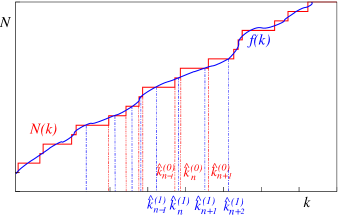
Figure 1: A continuous function $f(k)$ that pierces every stair step of the spectral staircase $N(k)$ of an 4 vertex linear chain graph. The intersection points $\hat{k}_{n}^{(1)}$ separate the momentum eigenvalues $\hat{k}_{n}^{(0)}$.

It is well known however, that following the behavior of the spectral staircase function (6) in such detail is generally a difficult task (see e.g. BaltesHilfe ). Luckily, quantum graphs allow an alternative approach, Opus ; Prima ; Anima , which is based on certain properties of their spectral determinant.

As shown in QGT2 ; Opus ; Prima ; Anima , the spectral determinant $\Delta(k)$ for quantum graphs is a finite order exponential sum,

$$\Delta(k)=1+e^{i2(L_{0}k-\pi\gamma_{0})}-\sum_{i=1}^{N_{\Gamma}}a_{i}e^{i2(L_{i}k-\pi\gamma_{i})},$$ (8)

with constant $a_{i}$, $L_{i}<L_{0}$ and $\gamma_{i}$. The order $N_{\Gamma}$ of the sum depends on the topology of the graph $\Gamma$. The explicit form (8) can obtained from imposing the boundary conditions on the wave function of the quantum particle moving on the network, e.g. by using the scattering quantization QGT2 ; Opus or the Bogomolny’s transfer operator Bogomolny2 methods. The roots of $\Delta(k)$ define the quantum spectrum of the momentum, $\Delta(\hat{k}^{(0)}_{n})=0$.

There are three key properties of the spectral determinant $\Delta(k)$ relevant for the following discussion. First, its roots as well as the roots of all of its derivatives are real Laguerre ; Levin . Second, there is exactly one root of its $j$th derivative, $\Delta^{(j)}(k)$, between every two neighboring roots of $\Delta^{(j+1)}(k)$. This implies that the zeroes of $\Delta(k)$ are interlaced by the zeroes of $\Delta^{\prime}(k)$, as required by (2), which in turn are interlaced by the zeroes of $\Delta^{\prime\prime}(k)$ and so on Laguerre ; Levin . Lastly, as shown in Anima , the higher is the order of the derivative, the more orderly is the behavior of the roots of $\Delta^{(j)}(k_{n}^{(j)})=0$ (Fig. 2). In fact, for any quantum graph system, there exists a finite integer $r$ (called the regularity degree of the graph in Anima , see also Bogomolny3 ,) such that the roots of $\Delta^{(r)}(k)$ can be interlaced by a periodic sequence of points

$$\hat{k}_{n}^{(r+1)}=\frac{\pi}{L_{0}}\left(n+\frac{1}{2}\right).$$ (9)

According to the criterion used in Opus ; Prima ; Anima , the regularity degree $r$ is the minimal integer for which the inequality

$$\sum_{i}\left|a_{i}\left(\frac{L_{i}}{L_{0}}\right)^{r}\right|<1$$ (10)

holds. Since $\left(\frac{L_{i}}{L_{0}}\right)<1$, this criterion allows to find a finite regularity degree for every quantum graph system using the coefficients of the spectral determinant (8).

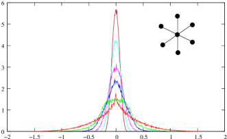
Figure 2: Histogram of the fluctuations of the roots of the 6-star graph of irregularity degree 5 and of the following 5 separating sequences, $\delta_{n}^{(0)}$, …, $\delta_{n}^{(5)}$. The initial spread of the fluctuations $\delta_{n}^{(0)}$ becomes progressively narrow for the higher values of $j$.

Hence, there exist $r+1$ almost periodic sequences of interest, $\hat{k}_{n}^{(j)}$, $j=0$, …, $r$, such that

$$\Delta^{(j)}\left(\hat{k}_{n}^{(j)}\right)=0,$$ (11)

and

$$\hat{k}_{n-1}^{(j)}<\hat{k}_{n}^{(j-1)}<\hat{k}_{n}^{(j)}.$$ (12)

The density functional for the $j$th sequence,

$$\rho^{(j)}(k)=\sum_{n}\delta\left(k-\hat{k}_{n}^{(j)}\right),$$ (13)

allows to pinpoint the exact location of $\hat{k}_{n}^{(j-1)}$ on the interval between $\hat{k}_{n}^{(j)}$ and $\hat{k}_{n-1}^{(j)}$,

$$\hat{k}_{n}^{(j-1)}=\int_{\hat{k}_{n-1}^{(j)}}^{\hat{k}_{n}^{(j)}}\rho^{(j-1)}(k)\,kdk,$$ (14)

for $\quad j=r+1,r-1,...,1$ and $n=1$,… . Since the roots of each $\Delta^{(j)}(k)$ form an almost periodic set Levin the density functional of each of the sequences $k^{(j)}_{n}$ can be expanded into an explicit harmonic series, which allows to evaluate the integral (14) explicitly for every $n$ and $j$.

The strategy that allows obtaining the separating sequences $\hat{k}_{n}^{(j)}$ and eventually getting the physical spectral sequence $\hat{k}_{n}^{(0)}$, follows directly from the bootstrapping (i.e. interlacing) property of the sequences (12) and the relationship (14). One first finds the sequence $\hat{k}_{n}^{(r)}$ starting from the periodic separators (9), then uses it to find $\hat{k}_{n}^{(r-1)}$, and so on. After $r$ steps of moving up the hierarchy the spectrum $\hat{k}_{n}^{(0)}$ is produced Anima .

Geometrically, this algorithm can illustrated using the integrated densities

$$N^{(j)}(k)=\sum_{n}\Theta\left(k-\hat{k}_{n}^{(j)}\right).$$ (15)

The separating property of the $j$th sequence $\hat{k}_{n}^{(j)}$ with respect to the sequence $\hat{k}_{n}^{(j-1)}$ implies that the staircase $N^{(1)}(k)$ “bootstraps” the staircase $N^{(0)}(k)$, whereas $N^{(2)}(k)$ bootstraps $N^{(1)}(k)$ and so on (see Fig.3, compare to Fig.1).

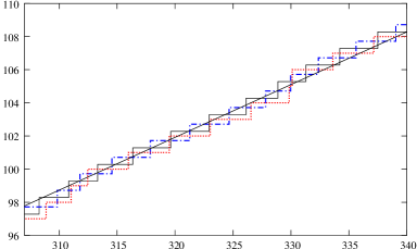
Figure 3: The bootstrapping of the spectral staircase (dotted line) by the $N^{(1)}$ staircase (dash-dotted line), bootstrapped in turn by the $N^{(2)}$ staircase (solid line) intersected by the Weyl’s average (straight line). Note that the $N^{(2)}$ staircase does not bootstrap the $N^{(0)}$. These graphs were obtained for the dressed 4 vertex linear chain graph Anima .

The final staircase $N^{(r)}(k)$ is pierced by the Weyl’s average

$$\bar{N}(k)=\frac{L_{0}}{\pi}k-\frac{1}{2}.$$ (16)

In the simplest case of $r=0$, the spectral points themselves can be separated from one another by a periodic sequence (9). Geometrically, this implies that the Weyl’s average pierces every stair step of the original $N(k)$, which guarantees the existence of periodic separators (9). Such networks were referred to as the “regular graphs” in Opus ; Prima ; Anima . The result of integration (3) in this case produces the quantum eigenvalues in the form of the periodic orbit series,

$$k_{n}=\frac{\pi}{L_{0}}n-\frac{2}{L_{0}}\sum_{p}\frac{A_{p}^{(0)}}{\omega^{(0)}_{p}}\sin\left(\frac{\omega^{(0)}_{p}}{2}\right)\sin\left(\omega^{(0)}_{p}n\right),$$ (17)

where $\omega^{(0)}_{p}=\pi L_{p}^{(0)}/L_{0}$. The first term in (17) gives the average behavior of the eigenvalue sequence, $\bar{k}_{n}=\frac{\pi n}{L_{0}}$, and the subsequent periodic orbit sum describes zero-mean fluctuations of $k_{n}$s around the average. It will be more convenient to describe the fluctuations in terms of the quantity $\delta_{n}^{(0)}=L_{0}\left(k-\bar{k}_{n}\right)/\pi$, $n=1,2,...$,

$$\delta^{(0)}_{n}=-\frac{2}{\pi}\sum_{p}\frac{A_{p}^{(0)}}{\omega^{(0)}_{p}}\sin\left(\frac{\omega^{(0)}_{p}}{2}\right)\sin\left(\omega^{(0)}_{p}n\right).$$ (18)

As demonstrated in Opus ; Prima ; Anima , if the sum (17) includes only the orbits that involve a certain fixed number $m$ of scatterings at the vertexes of the graph, it produces the $m$th order approximation to the exact value of $k_{n}$ for each $n$.

III Eigenvalue distribution for regular graphs

Let us first study the spectral fluctuation statistics for the regular graphs based on the expansion (17). The transition to statistical description of the sequence $\delta_{n}^{(0)}$, $n=1,2,...$, can be made based on the properties of the sequence of the remainders

$$x_{n}=\left[\alpha n\right]_{\mathop{\rm mod}1},\ n=1,2,...,$$ (19)

It is a well known number-theoretic result Karatsuba ; Kuipers that the sequence (19) is uniformly distributed over the interval $x_{n}\in\left[0,1\right]$ for any irrational number $\alpha$.

For every periodic orbit $p$ in (18), the frequency $\omega^{(0)}_{p}$ is defined as

$$\omega^{(0)}_{p}=m^{(0)}_{p,1}\Omega_{1}+...+m^{(0)}_{p,N_{B}}\Omega_{N_{B}}=\left\langle\vec{m}^{(0)}_{p},\vec{\Omega}_{p}\right\rangle,$$ (20)

where $\Omega_{i}=\pi l_{i}/L_{0}$ are the “bond frequencies” defined by the bond lengths $l_{i}$, $\sum_{i}\Omega_{i}=1$, and the vector $\vec{m}^{(0)}_{p}=(m^{(0)}_{p,1},...,m^{(0)}_{p,N_{B}})$ gives the number of times the orbit $p$ passes over the bond $i$. Considering that for every $\omega^{(0)}_{p}$ the function $\sin(\omega^{(0)}_{p}n)$ can be reduced to a combination of basic harmonics of $\Omega_{i}n$, one concludes that in the generic case in which every $l_{i}/L_{0}$ is an irrational number, the phases

$$x_{i,n}=\left[\Omega_{i}n\right]_{\mathop{\rm mod}2\pi}.$$ (21)

in each term in (20) will generate random outputs, uniformly distributed in the interval $[0,2\pi]$. Hence, in the context of studying the statistical properties of the eigenvalue sequence, the argument of every factor $\sin(\omega^{(0)}_{p}n)$ in (17) can be treated as a function

$$\sin\left(\omega^{(0)}_{p}n\right)\rightarrow\sin\left(m^{(0)}_{p,1}x_{1}+...+m^{(0)}_{p,N_{B}}x_{N_{B}}\right)=\sin\left(\vec{m}^{(0)}_{p}\vec{x}\right),$$ (22)

of $N_{B}-1$ independent random variables $x_{i}$, that are distributed in the interval $[0,2\pi]$. Hence the set of the deviations of the eigenvalues from the average is statistically described by a series or random inputs corresponding to the periodic orbit expansion (18)

$$\delta_{x}^{(0)}=-\frac{2}{\pi}\sum_{p}\frac{A_{p}^{(0)}}{\omega^{(0)}_{p}}\sin\left(\frac{\omega^{(0)}_{p}}{2}\right)\sin\left(\vec{m}^{(0)}_{p}\vec{x}\right).$$ (23)

The maximal amplitude of an input corresponding to a periodic orbit $p$ coincides with the amplitude of the same orbit’s contribution into the exact periodic orbit sum (17).

It is now a straightforward task to obtain the distribution of $\delta_{n}^{(0)}$ via

$$P_{\delta}^{(0)}\left(\delta^{(0)}\right)=\int_{0}^{2\pi}...\int_{0}^{2\pi}\delta\left(\delta^{(0)}+\sum_{p}C_{p}^{(0)}\sin\left(\vec{m}^{(0)}_{p}\vec{x}\right)\right)\prod_{i=1}^{N_{B}-1}\frac{dx_{i}}{2\pi}.$$ (24)

where

$$C_{p}^{(0)}=\frac{2}{\pi}\frac{A_{p}^{(0)}}{\omega^{(0)}_{p}}\sin\left(\frac{\omega^{(0)}_{p}}{2}\right).$$ (25)

Using the exponential representation of the $\delta$-functional, one has

$$P_{\delta}^{(0)}\left(\delta^{(0)}\right)=\int dke^{ik\delta^{(0)}}F_{\delta}^{(0)}\left(k,C_{p}^{(0)}\right),$$ (26)

where the characteristic function $F_{\delta}^{(0)}\left(k,C_{p}^{(0)}\right)$ is defined explicitly via the periodic orbits and graph parameters,

$$F_{\delta}^{(0)}\left(k,C_{p}^{(0)}\right)=\int_{0}^{2\pi}...\int_{0}^{2\pi}e^{ik\sum_{p}C_{p}^{(0)}\sin\left(\vec{m}^{(0)}_{p}\vec{x}\right)}\prod_{i=1}^{N_{B}-1}\frac{dx_{i}}{2\pi}.$$ (27)

As in the case of the series expansion for $k_{n}$, a finite order ($m$th) correction to the exact result is obtained by considering the orbits that involve the same number $|m^{(0)}_{p}|=m^{(0)}_{p,1}+...+m^{(0)}_{p,N_{B}}$ of vertex scatterings.

In general, the statistical properties of a spectral quantity $z_{n}$ that has a periodic orbit series expansion

$$z_{n}^{(0)}=f^{(0)}_{z}-\sum_{p}c_{p}^{(0)}\cos\left(\omega^{(0)}_{p}n+\varphi^{(0)}_{p}\right),$$ (28)

where $\varphi^{(0)}_{p}$ is an $n$-independent phase and $f^{(0)}_{z}$ is a shift term (see below), are described by the random sequence

$$z_{x}^{(0)}=f^{(0)}_{z}-\sum_{p}c_{p}^{(0)}\cos\left(\vec{m}^{(0)}_{p}\vec{x}+\varphi^{(0)}_{p}\right).$$ (29)

The corresponding characteristic function of probability distribution for $z$ will have the form

$$F_{z}^{(0)}(k)=\int_{0}^{2\pi}...\int_{0}^{2\pi}e^{ik\sum_{p}c_{p}^{(0)}\cos\left(\vec{m}^{(0)}_{p}\vec{x}+\varphi^{(0)}_{p}\right)}dx,$$ (30)

where $dx=\prod_{i=1}^{N_{B}-1}\frac{dx_{i}}{2\pi}$.

Another case of spectral characteristics that can be treated by this approach is provided e.g. by the separation between two eigenvalues, $k_{n+m}$ and $k_{n}$, for a fixed $m$. This quantity is defined by the expansion

$$s_{n,m}^{(0)}=\frac{\pi}{L_{0}}m-\sum_{p}D_{p,m}^{(0)}\cos\left(\omega^{(0)}_{p}n+\omega^{(0)}_{p}\frac{m}{2}\right),$$ (31)

with

$$D_{p,m}^{(0)}=\frac{4}{L_{0}}\frac{A_{p}^{(0)}}{\omega^{(0)}_{p}}\sin\left(\frac{\omega^{(0)}_{p}}{2}\right)\sin\left(\frac{\omega^{(0)}_{p}m}{2}\right),$$ (32)

which gives rise to the random series

$$s_{m,x}^{(0)}=\frac{\pi m}{L_{0}}-\sum_{p}D_{p}^{(0)}\cos\left(\vec{m}^{(0)}_{p}\vec{x}-\frac{m\omega^{(0)}_{p}}{2}\right).$$ (33)

The distribution of $s_{m}^{(0)}$ can be obtained as

$$P_{s_{m}}^{(0)}\left(s\right)=\int dke^{ik\left(s-\frac{\pi m}{L_{0}}\right)}F_{s_{m}}^{(0)}\left(k,D_{p,m}^{(0)}\right)$$ (34)

where $F_{s_{m}}^{(0)}\left(k,D_{p,m}^{(0)}\right)$ is defined according to (30). In the case $m=1$, these formulae describe the nearest neighbors distribution. Clearly, for the difference between the fluctuations themselves, $\sigma_{n,m}^{(0)}=\delta_{n+m}-\delta_{n}$, the distribution is $P_{\sigma_{m}}^{(0)}(\sigma)=P_{s_{m}}^{(0)}\left(s+\frac{\pi m}{L_{0}}\right)$.

One could also study the mean of the two neighboring deviations, $\xi_{n}^{(0)}=\left(\delta_{n}^{(0)}+\delta_{n-1}^{(0)}\right)/2$. This characteristics can be used to generate the separators directly from $k_{n}^{(0)}$, $k_{n}^{(1)}=n+\xi_{n}^{(0)}$ independently of the properties of the spectral determinant. The corresponding series has the expansion coefficients

$$E_{p}^{(0)}=\frac{1}{\pi}\frac{A_{p}^{(0)}}{\omega^{(0)}_{p}}\sin\left(\omega^{(0)}_{p}\right)$$ (35)

and phases $\varphi^{(0)}_{p}=\frac{\pi}{2}-\frac{\omega^{(0)}_{p}}{2}$. The energy fluctuations, $\delta E_{n}$, have the expansion coefficients

$$H_{p}^{(0)}=\frac{2\pi}{L_{0}^{2}}\frac{A_{p}^{(0)}}{\omega^{(0)}_{p}}\left(\frac{2}{\omega^{(0)}_{p}}\sin\left(\frac{\omega^{(0)}_{p}}{2}\right)-\cos\frac{\omega^{(0)}_{p}}{2}\right),$$ (36)

phases $\varphi^{(0)}_{p}=0$ and $f_{E}=\frac{\pi^{2}}{12L_{0}^{2}}$, etc.

These quantities can be used to find the periodic orbit expansions for higher order statistics, such as the correlator $\left\langle\delta_{n}^{(0)}\delta_{n+m}^{(0)}\right\rangle$ or the autocorrelation function,

$$R_{2}(x)=\frac{\pi^{2}}{L_{0}^{2}}\left\langle\rho\left(k+\frac{x}{2}\right)\rho\left(k-\frac{x}{2}\right)\right\rangle=\frac{\pi}{L_{0}}\lim_{N\rightarrow\infty}\frac{1}{N}\sum_{n=1}^{N}\sum_{m\neq 0}\delta\left(k_{n+m}-k_{n}+x\right).$$ (37)

which defines the probability to find a new level at a distance $x\neq 0$ from a given old one, whether or not these levels are nearest neighbors. The Fourier image of $R_{2}(x)$, the form factor, $K_{2}(\tau)$ is given by

$$K_{2}(\tau)=\frac{\pi}{L_{0}}\lim_{N\rightarrow\infty}\frac{1}{N}\sum_{n=1}^{N}\sum_{m=1}^{N}e^{i\left(k_{n+m}-k_{n}\right)\tau}=\frac{\pi}{L_{0}}\left\langle\sum_{m}e^{-i\left(k_{n+m}-k_{n}\right)\tau}\right\rangle_{n}.$$ (38)

For the regular graphs with $k_{n}$ given by (17), the averaging over $n$ can be performed via

$$K_{2}(\tau)=\frac{\pi}{L_{0}}\lim_{N\rightarrow\infty}\frac{1}{N}\sum_{n=1}^{N}\sum_{m}e^{i\left(-\frac{\pi}{L_{0}}m+\sum_{p}D_{p,m}^{(0)}\cos\left(\omega^{(0)}_{p}\left(n+\frac{m}{2}\right)\right)\right)\tau}$$ (39)

$$=\frac{\pi}{L_{0}}\sum_{m}e^{-i\frac{\pi m}{L_{0}}\tau}\int e^{i\sum_{p}\tau D_{p,m}^{(0)}\cos\left(\vec{m}^{(0)}_{p}\vec{x}+\omega^{(0)}_{p}\frac{m}{2}\right)}\prod_{i}\frac{dx_{i}}{2\pi}.$$ (40)

The latter integral is defined by (34), so

$$K_{2}(\tau)=\frac{\pi}{L_{0}}\sum_{m=1}^{\infty}e^{-i\frac{\pi m}{L_{0}}\tau}F_{s_{m}}^{(0)}\left(\tau,D_{p,m}^{(0)}\right).$$ (41)

Formula (41) can also be obtained directly from (38) by averaging over the random variable $s_{m}^{(0)}$ using the distribution (34),

$$K_{2}(\tau) = \frac{\pi}{L_{0}}\left\langle\sum_{m}e^{-i\left(k_{n+m}-k_{n}\right)\tau}\right\rangle_{n}=\frac{\pi}{L_{0}}\sum_{m}\left\langle e^{-is_{m}^{(0)}\tau}\right\rangle_{s_{m}}.$$

Hence $R_{2}(x)$ is given by

$$R_{2}(x)=\frac{\pi}{L_{0}}\sum_{m}\int e^{i\tau\left(x-\frac{\pi m}{L_{0}}\right)}F_{s_{m}}^{(0)}\left(\tau,D_{p,m}^{(0)}\right)d\tau=\frac{\pi}{L_{0}}\sum_{m}P_{s_{m}}^{(0)}(x),$$ (42)

as the sum of the probabilities that the two eigenvalues separated by the interval $x$ have $m-1$ other eigenvalues in-between.

It should be emphasized that all the probability distributions above are obtained in the context of the standard periodic orbit theory framework. All the distributions for the regular level fluctuations derived in this section are closed, self contained expressions, defined in terms of the periodic orbits and graph parameters. It is also important to notice that the statistical properties of some (especially some regular) quantum graphs, despite being strongly stochastic in the classical regime, deviate from the universal Wignerian distributions predicted by the RMT. However these cases, as well as the irregular graphs discussed below, are equally well described via statistical description of the periodic orbit expansion series for the spectral sequences.

IV Spectral expansions for irregular graphs

As mentioned in the Section II, one can find the roots of $\Delta^{(j-1)}(k)$ by using the density $\rho^{(j)}(k)$ and the separators $\hat{k}_{n}^{(j)}$ in formula (14), which yields

$$\hat{k}_{n}^{(j-1)}=\hat{k}_{n}^{(j)}N^{(j-1)}\left(\hat{k}_{n}^{(j)}\right)-\hat{k}_{n-1}^{(j)}N^{(j-1)}\left(\hat{k}_{n-1}^{(j)}\right)-\int_{\hat{k}_{n-1}^{(j)}}^{\hat{k}_{n}^{(j)}}N^{(j-1)}(k)dk.$$ (43)

Every staircase function $N^{(j)}(k)$ can be decomposed into the average and the oscillating parts, $N^{(j)}(k)=\bar{N}^{(j)}(k)+\delta N^{(j)}(k)$, where the average integrated density for every $j$ is

$$\bar{N}^{(j)}(k)=\frac{L_{0}}{\pi}k-\frac{1}{2}=\bar{N}(k).$$ (44)

The bootstrapping (12) of $\hat{k}_{n}^{(j-1)}$ by $\hat{k}_{n}^{(j)}$ (or $N^{(j-1)}(k)$ by $N^{(j)}(k)$, see Fig.3) implies that

$$N^{(j-1)}\left(\hat{k}_{n}^{(j)}\right)=n.$$ (45)

Using (44), (45) and writing $\hat{k}_{n}^{(j)}$ in the form

$$\hat{k}_{n}^{(j)}=\frac{\pi}{L_{0}}\left(n+\delta_{n}^{(j)}\right),$$ (46)

we get for the $j-1$ generation of the separators

$$\hat{k}_{n}^{(j-1)}=\frac{\pi n}{L_{0}}+\frac{1}{2}\frac{\pi}{L_{0}}\left(\delta_{n}^{(j)}-\delta_{n-1}^{(j)}\right)-\frac{1}{2}\frac{\pi}{L_{0}}\left((\delta_{n}^{(j)})^{2}-(\delta_{n-1}^{(j)})^{2}\right)-\int_{\hat{k}_{n-1}^{(j)}}^{\hat{k}_{n}^{(j)}}\delta N^{(j-1)}(k)~{}dk.$$ (47)

The harmonic series expansion for $\delta N^{(j)}(k)$,

$$\delta N^{(j)}(k)=\frac{1}{\pi}\mathop{\rm Im}\sum_{p}A_{p}^{(j)}e^{iL^{(j)}_{p}k},$$ (48)

allows to compute the integral in (49) explicitly, which yields the fluctuating part of $\hat{k}_{n}^{(j-1)}$ via an expansion similar to (18),

$$\delta_{n}^{(j-1)}=f^{(j-1)}_{\delta}\left(\delta_{n}^{(j)},\delta_{n-1}^{(j)}\right)-\sum_{p}C_{p}^{(j-1)}\left(\delta_{n}^{(j)},\delta_{n-1}^{(j)}\right)\sin\left(\omega^{(j-1)}_{p}n+\varphi^{(j-1)}_{p}\left(\delta_{n}^{(j)},\delta_{n-1}^{(j)}\right)\right),$$ (49)

where now the expansion coefficients,

$$C_{p}^{(j-1)}=\frac{2}{\pi}\frac{A_{p}^{(j-1)}}{\omega^{(j-1)}_{p}}\sin\frac{\omega^{(j-1)}_{p}}{2}\allowbreak\left(\delta_{n}^{(j)}-\delta_{n-1}^{(j)}+1\right),$$ (50)

the “zero shift” term,

$$f^{(j-1)}_{\delta}=\frac{1}{2}\left(\delta_{n}^{(j)}-\delta_{n-1}^{(j)}\right)-\frac{1}{2}\left((\delta_{n}^{(j)})^{2}-(\delta_{n-1}^{(j)})^{2}\right),$$ (51)

and the phases,

$$\varphi^{(j-1)}_{p}=\frac{\delta_{n}^{(j)}+\delta_{n-1}^{(j)}-1}{2}\omega^{(j-1)}_{p},$$ (52)

are functions of the fluctuations $\delta_{n}^{(j)}$ and $\delta_{n-1}^{(j)}$ on the previous level of the hierarchy. In the particular case when $r=0$, $\delta_{n}^{(1)}=\delta_{n-1}^{(1)}=1/2$, (49) coincides with the oscillating part of (17).

The equation (49) shows that the fluctuations $\delta_{n}^{(j-1)}$ have two sources. In addition to the oscillations induced by the periodic orbit sum in (49), there are also oscillating contributions produced by $\delta_{n}^{(j)}$ and $\delta_{n-1}^{(j)}$ that bring in the oscillations from all the previous levels of the hierarchy. This equation will later be used to produce the exact statistical distribution for the fluctuations $\delta_{n}^{(j)}$ at each level of the hierarchy.

As an example of a case where the coefficients $A^{(j)}_{p}$ can be obtained directly, one can use a simple example of a 2-bond regular graph, discussed in Prima ; Opus . Although the 2-bond graph is a strictly regular system, which does not require auxiliary separating sequences for obtaining its spectrum, it is nevertheless useful to use this case to have an immediate illustration of the explicit form of the coefficients $A^{(j)}_{p}$.

As shown in Nova ; Prima ; Opus , the spectral equation in this case has the form

$$\sin((l_{1}+l_{2})k)-r\sin((l_{1}-l_{2})k)=0,$$ (53)

where $r$ is the reflection coefficient at the middle vertex and $l_{1}$ and $l_{2}$ are the two bond lengths. This equation was obtained in Nova ; Prima ; Opus using scattering quantization method QGT1 ; QGT2 as $\Delta(k)=\det(1-S(k))=0$, where scattering matrix $S(k)\equiv S^{(0)}(k)$ in this case is

$$S^{(0)}(k)=\pmatrix{0&-e^{il_{1}k}&0&0\cr re^{il_{1}k}&0&0&te^{il_{2}k}\cr te^{il_{1}k}&0&0&-re^{il_{2}k}\cr 0&0&-e^{il_{2}k}&0}.$$ (54)

The unitarity of $S(k)$ is guaranteed by the “flux conservation” relationship between the reflection and the transmission coefficient, $t^{2}+r^{2}=1$. The expansion of the spectral determinant QGT1 ; QGT2 ; Opus , yields the exact periodic orbit expansion for $N(k)$,

$$N(k)=\bar{N}(k)-\frac{1}{\pi}{\rm Im}\sum_{p,\nu}\frac{1}{\nu}\left[(-1)^{\chi(p)}t^{2\tau(p)}r^{\sigma(p)}\right]^{\nu}\,e^{i\nu L_{p}k}$$ (55)

where $\nu$ is the multiple traversal index for the prime periodic trajectory $p$, $\sigma(p)$ and $2\tau(p)$ are the numbers of reflections and transmissions for $p$ at the middle vertex, and the factor $(-1)^{\chi(p)}$ defines the Maslov index Nova . The action length of $p$ is $L_{p}=m_{p,1}l_{1}+m_{p,2}l_{2}$, according to the number of times, $m_{p,1}$ and $m_{p,2}$, it traverses the bonds $l_{1}$ and $l_{2}$. One can notice that the equation for the separating points $\hat{k}^{(1)}_{n}$,

$$\cos((l_{1}+l_{2})k)-r\omega\cos((l_{1}-l_{2})k)=0,$$ (56)

where $\omega=(l_{1}-l_{2})/(l_{1}+l_{2})<1$, reduces to the original equation (53), if $r\rightarrow r^{(1)}=\omega r$ and $l_{1}k\rightarrow l_{1}k+\frac{\pi}{2}$. Therefore, the expansion for $N^{(1)}(k)$ can be obtained from $\det(1-S^{(1)}(k))$, where unitary matrix $S^{(1)}(k)$ is obtained via a two parameter deformation of the unitary matrix $S^{(0)}(k)$,

$$S^{(1)}=\pmatrix{0&-e^{il_{1}k+\frac{\pi}{2}}&0&0\cr r^{(1)}e^{il_{1}k+\frac{\pi}{2}}&0&0&t^{(1)}e^{il_{2}k}\cr t^{(1)}e^{il_{1}+\frac{\pi}{2}}&0&0&-r^{(1)}e^{il_{2}k}\cr 0&0&-e^{il_{2}k}&0}.$$ (57)

with $r^{(1)}=\omega r$ and $t^{(1)}=\sqrt{1-\left(r^{(1)}\right)^{2}}$. The weight coefficients $A^{(1)}_{p}$ are now explicitly defined via the products of the matrix elements of $S^{(1)}(k)$, just as the $A^{(0)}_{p}$ coefficients were defined via $S^{(0)}(k)$ in (55).

Clearly, all even order derivatives of the spectral equation (53) for $j=2w$ have the form $\sin((l_{1}+l_{2})k)-r\omega^{2w}\sin((l_{1}-l_{2})k)=0$, so with the replacement $r^{(2w)}=\omega^{(2w)}r$, $t^{(2w)}=\sqrt{1-\left(r^{(2w)}\right)^{2}}$, the form of the coefficients $A^{(2w)}_{p}$ is structurally same as the one found in (55). The odd degree derivatives $A^{(2w+1)}_{p}$ are produced by the expansion of the determinant $\det(1-S^{(2w+1)}(k))$ analogous to (57). It should be mentioned however, that in general the task of obtaining the exact form of the coefficients $A^{(j)}_{p}$ and frequencies $\omega^{(j)}_{p}$ for $j\neq 0$ is not as straightforward as in this simple case and requires a more detailed analysis. In particular, the harmonic expansions such as (49) may include bond combinations that do not correspond to connected periodic orbits.

Using the expansion for the fluctuations $\delta^{(j-1)}_{n}$, one can find the harmonic expansions for other spectral characteristics. For example, the $m$-neighbor difference, $s_{n,m}^{(j-1)}=m+\delta_{n+m}^{(j-1)}-\delta_{n}^{(j-1)}$, the expansion is

$$s_{n,m}^{(j-1)}=f^{(j-1)}_{s}\left(s_{n-1,m}^{(j)},s_{n,m}^{(j)},s_{n,m-1}^{(j)},\xi_{n}^{(j)}\right)+\sum_{p}D_{p,m}^{(j-1)}\cos\left(n\omega^{(j-1)}_{p}+\varphi^{(j-1)}_{p}\right),$$ (58)

where

$$f^{(j-1)}_{s}=s_{n,m}^{(j)}+\frac{1}{2}\left(s_{n,m}^{(j)}-s_{n,m-1}^{(j)}\right)\left(2m-s_{n,m}^{(j)}-s_{n-1,m}^{(j)}\right)+\xi_{n}^{(j)}\left(s_{n-1,m}^{(j)}-s_{n,m}^{(j)}\right)$$ (59)

and $\xi_{n}^{(j)}=\frac{1}{2}\left(\delta_{n}^{(j)}+\delta_{n-1}^{(j)}\right)$. The harmonic expansion coefficients in this case are

$$D_{p,m}^{(j-1)}=\frac{A_{p}^{(j-1)}}{\omega^{(j-1)}_{p}}\Big{(}\sin^{2}\frac{\omega^{(j-1)}_{p}}{2}s_{n,m}^{(j)}+\sin^{2}\frac{\omega^{(j-1)}_{p}}{2}s_{n-1,m}^{(j)}$$ (60)

$$-2\left(\sin\frac{\omega^{(j-1)}_{p}}{2}s_{n,m}^{(j)}\sin\frac{\omega^{(j-1)}_{p}}{2}s_{n-1,m}^{(j)}\right)\cos\frac{\omega^{(j-1)}_{p}}{2}\left(2s_{n,m-1}^{(j)}-s_{n,m}^{(j)}-s_{n-1,m}^{(j)}\right)\Big{)}^{1/2}$$ (61)

In case $m=1$ the system of equations (58) yields the nearest neighbor distances between of the $j-1$ level separators.

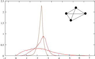
Figure 4: Histogram of the nearest neighbor separations $s^{(0)}_{n}$ (bottom distribution), $s^{(1)}_{n}$ and $s^{(2)}_{n}$ (top distribution) for the fully connected quadrangle graph (top right corner) of the irregularity degree 3, obtained for 80,000 roots of the corresponding spectral equations. The maximal nearest neighbor separation for $j=0$ in this case is $s_{max}=8.68$, while regular cell size is $\pi/S_{0}=2.28$.

The nearest neighbor average, $\xi^{(j)}_{n}$, that appears e.g. in (61) has the expansion

$$\xi_{n}^{(j-1)}=f^{(j-1)}_{\xi}\left(s_{n}^{(j)},s_{n-1}^{(j)},\xi_{n}^{(j)}\right)-\sum_{p}E_{p}^{(j-1)}\left(s_{n}^{(j)},s_{n-1}^{(j)}\right)\sin\left(\omega^{(j-1)}_{p}n+\varphi^{(j-1)}_{p}\right),$$ (62)

where

$$f^{(j-1)}_{\xi} = -\frac{1}{4}\frac{L_{0}^{2}}{\pi^{2}}\left(s_{n}^{(j)}+s_{n-1}^{(j)}-\frac{2\pi}{L_{0}}\right)\left(s_{n}^{(j)}-\frac{2\pi}{L_{0}}+\frac{2\pi}{L_{0}}\xi_{n-1}^{(j)}\right)$$

$$E_{p}^{(j-1)} = \frac{1}{L_{0}}\frac{A_{p}^{(j-1)}}{\omega^{(j-1)}_{p}}\sin\frac{L^{(j-1)}_{p}}{2}\left(s_{n}^{(j)}+s_{n-1}^{(j)}\right)$$

$$\varphi^{(j-1)}_{\xi,p} = \left(\frac{L_{0}}{2}s_{n}^{(j)}+\xi_{n-1}^{(j)}-\frac{3}{2}\right)\omega^{(j-1)}_{p}.$$

The expansions of the kind (49), (58) and (62), provide an exact description of the propagation of the spectral characteristics across the hierarchy in terms of the geometry of the graph. For the graphs of high degree of irregularity, the equations (49), (58), (62), etc., can be considered as discretizations of nonlinear differential equations for continuous functions $\delta_{n}^{(j)}\sim\delta(n,j)$, $s_{n,m}^{(j)}\sim s_{m}(n,j)$, $\xi_{n}^{(j)}\sim\xi(n,j)$, etc.

V Fluctuation Statistics

As demonstrated in the previous section, the fluctuations $z_{n}^{(j)}$ (e.g. (49), (58), (62)) at the $j$th level of the hierarchy depend on the fluctuations on all the previous levels as well as on the oscillations introduced by the harmonic terms at the level $j$,

$$z_{n}^{(j-1)}=f^{(j-1)}\left(z_{n}^{(j)}\right)-\sum_{p}c_{p}^{(j-1)}\left(z_{n}^{(j)}\right)\cos\left(\omega^{(j-1)}_{p}n+\varphi^{(j-1)}_{p}\left(z_{n}^{(j)}\right)\right),$$ (63)

As in the regular case considered in Chapter III, probabilistic description of the sequence $z^{(j)}$ at each $j$ is obtained by considering $z^{(j)}$ as a function of a random vector $\vec{x}$, generated by the sequence $x_{i}=\left[\Omega_{i}n\right]_{\mathop{\rm mod}2\pi}$,

$$z_{x}^{(j-1)}=f^{(j-1)}\left(z_{x}^{(j)}\right)-\sum_{p}c_{p}^{(j-1)}\left(z_{x}^{(j)}\right)\cos\left(\vec{m}^{(j-1)}_{p}\vec{x}+\varphi^{(j-1)}_{p}\left(z_{x}^{(j)}\right)\right).$$ (64)

Since the index $n$ and the “bond frequencies” $\Omega_{i}$ are the same for all the $z_{n}^{(j)}$ expansions across the hierarchy, the random variable $\vec{x}$ is the same in all the harmonic expansion terms in the stochastic series (64), $j=0,\ ...,\ r$. This implies however, that unlike the regular case, the harmonic oscillations at the higher levels of the hierarchy ($j<r$) are not the only source of randomness in the series (64). Additional “noise” at the level $j$ is injected into the equation (64) by the variables $z_{x}^{(j)}$, that introduce the fluctuations from all the previous levels of the hierarchy into its $j-1$ level. The expansions (64) allow to obtain the probability distributions for each of the $z^{(j)}$s from

$$P_{z}^{(j-1)}(z^{(j-1)})=\int\delta\left(z^{(j-1)}-z^{(j-1)}\left({z_{x}^{(j)}}\left({z_{x}^{(j+1)}}(...),x\right),x\right)\right)dx,$$ (65)

where $dx=\prod\limits_{i}\frac{dx_{i}}{2\pi}$. The “nested” structure of the $z_{x}^{(j-1)}$ in (65) can be unfolded in the form

$$P_{z}^{(j-1)}(z^{(j-1)}) = \int\delta\left(z^{(j-1)}-z^{(j-1)}\left({z_{x}^{(j)},x}\right)\right)$$ (68)

$$\times\delta\left(z_{i}^{(j)}-z_{i}^{(j)}\left({z_{x}^{(j+1)},x}\right)\right)$$

$$...\times\delta\left(z_{i}^{(r)}-z_{i}^{(r)}(x)\right)\prod_{j}\prod_{i}z^{(j)}_{i}dx.$$

in which the chain of the delta functionals above can be understood as the conditional probability densities for obtaining the value $z^{(j-1)}$, given the values of $\vec{x}$ and $z^{(j)}$, $z^{(j+1)}$, … , $z^{(r)}$. Here the index $i$ runs over the number of the elements $z^{(j)}_{i}$ that appear in the expansion (63) of the corresponding quantity $z^{(j-1)}$. For example, the expansion of $\delta^{(j-1)}_{n}$ depends on $\delta^{(j)}_{n-1}$ and $\delta^{(j)}_{n}$, so in this case index $i$ takes two values, $i=1,2$. In the following this index will be omitted for conciseness of notations.

The hierarchical organization of the fluctuations suggests a natural way of approximate evaluation of the expression (68). Since for every $j$ the function $z^{(j)}_{x}$ is a complex, rapidly oscillating function of $x$, and since every $z^{(j-1)}$ characteristics depends explicitly only on the previous level sequence $z^{(j)}$, it is natural to consider a simple approximation to (68), in which $z^{(j)}$ in the equations (64) are treated as independent random variables distributed according to $P_{z}^{(j)}$,

$$P_{z}^{(j-1)}(z^{(j-1)})=\int\delta\left(z^{(j-1)}-z^{(j-1)}\left({z^{(j)},x}\right)\right)P^{(j)}_{z}dz^{(j)}dx.$$ (69)

A more formal and elaborate argument that will not be discussed here in detail is based on inverting the dependence $z^{(j-1)}=z^{(j-1)}(x)$ for each $j$ in the arguments of the delta functionals in (68) (i.e. in effect using Bayes relationships $P(z|x)P(x)=P(x|z)P(z)$). It is clear that due to the complex oscillatory behavior of the expansions $z^{(j-1)}(x)$, one can approximate each of the $P_{z}^{(j)}(x|z)$ distributions by a uniform distribution, which effectively corresponds to introducing separate $x$-variables for each level $j$, and leaves, after intermediate integrations, the distribution $P^{(j)}_{z}$ in (69).

Such approach takes a natural advantage the hierarchical organization of the fluctuations produced by the sequences $z^{(j)}$. Since the distribution $P_{z}^{(r)}$ at the regular level can be computed directly, the distribution $P_{z}^{(r-1)}$, $P_{z}^{(r-2)}$, …, can be computed in sequence, from the previous levels of the hierarchy to the next. The final distributions $P_{z}^{(0)}$ will apply to the physical characteristics of the spectrum.

As an example, one can consider the transition from the level $j$ to the level $j-1$ of the distributions for the deviations from the average. The $j$th level fluctuations $\delta_{n}^{(j)}$ and $\delta_{n-1}^{(j)}$ in (49), can now be considered as random variables, $\delta_{1}$ and $\delta_{2}$, distributed according to $P_{\delta}^{(j)}\left(\delta\right)$. Hence for the density $P_{\delta}^{(j-1)}(\delta)$ one can write

$$P_{\delta}^{(j-1)}\left(\delta\right)=\int d\delta_{1}d\delta_{2}dxP_{\delta}^{(j)}\left(\delta_{1}\right)P_{\delta}^{(j)}\left(\delta_{2}\right)\delta{\Bigg{(}}\delta-f^{(j-1)}_{\delta}\left(\delta_{1}^{(j)},\delta_{2}^{(j)}\right)$$ (70)

$$+\sum_{p}C_{p}^{(j-1)}\left(\delta_{1}^{(j)},\delta_{2}^{(j)}\right)\sin\left(\vec{m}^{(j-1)}_{p}\vec{x}+\varphi^{(j-1)}_{p}\left(\delta_{1}^{(j)},\delta_{2}^{(j)}\right)\right){\Bigg{)}}.$$ (71)

Exponentiation of the delta function produces

$$P^{(j-1)}(\delta)=\int dke^{ik\delta}\left\langle F_{\delta}^{(j-1)}\left(k,C_{p}^{(j-1)}\right)\right\rangle_{\Omega^{(j)}},$$ (72)

where the function

$$F_{\delta}^{(j-1)}(k)=\int_{0}^{2\pi}...\int_{0}^{2\pi}e^{ik\sum_{p}C_{p}^{(j-1)}\left(\delta_{1},\delta_{2}\right)\sin\left(\vec{m}^{(j-1)}_{p}\vec{x}+\varphi^{(j-1)}_{p}\right)}dx,$$ (73)

produced by the integral over $x_{i}$s is reminiscent of the (27). The parenthesis $\left\langle\ast,\ast\right\rangle_{\Omega^{(j)}}$ denote averaging of the $F_{\delta}^{(j)}(k)$ with the weight

$$\Omega^{(j)}(\delta^{(j)}_{1},\delta^{(j)}_{2},k)=e^{-ikf^{(j-1)}_{\delta}\left(\delta_{1}^{(j)},\delta_{2}^{(j)}\right)}P_{\delta}^{(j)}\left(\delta_{1}\right)P_{\delta}^{(j)}\left(\delta_{2}\right),$$ (74)

which corresponds to averaging over the “separator disorder”, which yields the characteristic function of the distribution (72). In case if $P_{\delta}^{(r+1)}=\delta\left(\delta^{(r+1)}-\frac{1}{2}\right)$ (ordered separators at $j=r$), one recovers the regular level distribution (26). For $j<r$, obtaining the probability distributions $P^{(j-1)}_{\delta}(\delta)$ for requires an additional averaging over the disorder produced by the fluctuating sequences of the separators $\hat{k}^{(j)}_{n}$.

The expression for other spectral characteristics have similar structure. In the case of the $m$-th neighbor separation statistics, the probability distribution for $s_{m}^{(j-1)}$ is given by

$$P_{m}^{(j-1)}(s)=\int e^{ik\left(s-m\right)}\left\langle F_{s_{m}}^{(j)}\right\rangle_{\Phi^{(j)}}dk,$$ (75)

where the “characteristic exponential” $F_{s_{m}}^{(j)}$ generated by the harmonic series $\delta s_{x,m}^{(j-1)}$ similarly to (73), is averaged with the weight

$$\Phi^{(j)}\left(s_{1},s_{2},s_{3},\xi\right)=e^{-if^{(j-1)}_{s}\left(s_{1},s_{2},s_{3},\xi\right)}P_{\xi}^{(j)}(\xi)P_{s_{m}}^{(j)}(s_{1})P_{s_{m}}^{(j)}(s_{2})P_{s_{m}}^{(j)}(s_{3}).$$ (76)

In the case if $m=1$ this yields the distributions for the nearest neighbor spacings. The resulting distributions can be used to compute the form factor, $K^{(j)}_{2}(\tau)$, the autocorrelation $R^{(j)}_{2}(x)$ function and so on.

VI Trigonometric sums and spectral universality

An important advantage of obtaining the statistical description of spectra in terms of the harmonic expansions, is that the well known universality features of the quantum chaotic systems (e.g. BGS ; ABS ) can now be analyzed within the context of the theory of trigonometric series and weakly dependent random variables (see Proxorov ; Revesz and references therein). As shown e.g. in Erdos ; SZ1 ; SZ2 ; Philipp ; Philipp2 ; Berkes1 ; Fukuyama ; Takahashi , under certain conditions separate terms of trigonometric (or more general Berkes ) series statistically behave as a set of weakly dependent random variables Kahane . This allows establishing analytically certain universal features for the distribution of their sums, e.g. the corresponding generalization of the central limit theorem.

It is well known (Erdos ; SZ1 ; SZ2 ; Philipp ; Philipp2 ; Berkes1 ; Fukuyama ; Takahashi ), that if the frequencies of the trigonometric series

$$f(x)=\sum_{k}c_{k}\cos(2\pi n_{k}x+\phi_{k})$$ (77)

increase sufficiently rapidly so that the “critical condition”,

$$\frac{n_{k+1}}{n_{k}}=1+\frac{\alpha_{k}}{\sqrt{k}},\ \ \alpha_{k}\rightarrow\infty$$ (78)

is satisfied, then a central limit theorem holds for the sum (77),

$$\frac{1}{\Delta_{K}}\sum_{k=1}^{K}c_{k}\cos(2\pi n_{k}x+\phi_{k})\rightarrow{\cal{N}}_{0,1},$$ (79)

where ${\cal{N}}_{0,1}$ is the standard normal distribution and $\Delta^{2}_{K}=\frac{1}{2}\sum_{k=1}^{K}c^{2}_{k}$.

Although the series (77) is much simpler than the spectral expansions studied in the context of the periodic orbit theory, similar result was previously observed in the physical literature. Based on the extensive numerical simulations, it was hypothesized in ABS that the fluctuations of the spectral staircase $\delta N(k)$ of ageneric quantum chaotic system are normally distributed with the standard deviation

$$\Delta_{\infty}=\frac{1}{2}\sum_{p}A^{2}_{p},$$ (80)

introduced in ABS via spectral rigidity, where $A_{p}$’s are the expansion coefficients (48) for $\delta N(k)$. In particular, this applies to the quantum graphs, for which there exists an exact periodic orbit expansion (48) for $\delta N(k)$. Although the fluctuations of the quantum graph spectrum are finite Anima , their distributions are typically well approximated by the Gaussian distribution (see Fig.2 and Fig.5 below), just as the finite range $P_{s}$ can approximated by the Wignerian distribution QGT2 (see Fig.4).

The explicit expansions (29) and (64) allow to extend the scope of the “central limit theorem for spectral fluctuations” of ABS hypothesis to a much wider range of spectral characteristics. For example, the probability distributions of the nearest neighbor average, $\xi_{n}^{(j-1)}$, shown in Fig. 5, which can be obtained from (62) as

$$P_{\xi}^{(j-1)}(\xi)=\int dk\,e^{ik\xi}\left\langle F_{\xi}^{(j)}\right\rangle_{\Upsilon_{\xi}^{(j)}}$$ (81)

with the weight

$$\Upsilon_{\xi}^{(j)}\left(s_{1},s_{2},\xi\right)=e^{-ikf^{(j-1)}_{\xi}\left(s_{1},s_{2},\xi\right)}P_{\xi}^{(j)}(\xi)P_{s}^{(j)}(s_{1})P_{s}^{(j)}(s_{2}),$$ (82)

are also well approximated by Gaussian distribution with the corresponding variance.

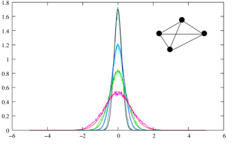
Figure 5: Histogram of the nearest neighbor average for the even levels of the hierarchy of the fully connected quadrangle graph of the irregularity degree 7, obtained for 80,000 roots of the corresponding spectral equations. The solid line in the background of each histogram represents a Gaussian fit with $\Delta$ given by the corresponding sum (80).

It is important to mention that although the condition (78) is required for the general proof of the central limit theorem (79), Erdos ; SZ1 ; SZ2 ; Philipp ; Fukuyama ; Takahashi , in some cases it is possible to establish the existence of limit distributions if (78) is violated (see e.g. Berkes1 ; Berkes2 ; Levizov ; Wang ). This is essential for the periodic orbit expansions, because lacunarity condition (78) generally may not hold for the prime periodic orbit spectrum of the quantum graphs and of more general systems. However extensive numerical and empirical evidence points on the existence of the corresponding limiting distributions ABS .

There are much fewer proved results about the probabilistic behavior of the multiple trigonometric series such as the spectral expansions (29) or (64) (see Gaposhkin1 ; Gaposhkin2 ; BerPhil ; Ulyanov ; Golubov ; Zygmund ; Wang and the references therein), specifically regarding the conditions required for convergence of their sums to the limiting distributions. Nevertheless, the proposed connection to the spectral theory clearly implies the existence of the limiting distributions for such expansions and points out the origins of the spectral universality BGS ; ABS from the perspective of the periodic orbit theory.

The nontrivial role of the transitions between the probability distributions at different levels of the hierarchy (such as (72) or (75)) can be seen on the example of the development of the nearest neighbor distributions (see Fig.4). Although the distribution at the regular level has overall Gaussian shape, the profile of the distributions $P^{(j)}_{s}(s)$ for $j>0$ becomes progressively closer to the Wignerian form.

VII Discussion

The method of obtaining the explicit semiclassical expansions for the individual spectral points outlined above is based on the possibility to tie the sequence of momentum eigenvalues, $k_{n}\equiv\hat{k}_{n}^{(0)}$, to a certain base, regular sequence $\hat{k}_{n}^{(r+1)}$ defined explicitly as a function of the index $n$. As shown in Anima , this can be done either directly, as in the case of the regular graphs, where the periodic sequence (83) is used to place the points $k_{n}$ into a system of periodic cells, or indirectly, as in the case of the irregular graphs, where a few auxiliary sequences, $\hat{k}_{n}^{(j)}$, are needed to complete the bootstrapping.

The system of the auxiliary sequences, $\hat{k}_{n}^{(j)}$, that links the base sequence $\hat{k}_{n}^{(r+1)}$ and the physical spectral sequence $\hat{k}_{n}^{(0)}$, together with the rule of transition from the $j$th to $j-1$th level, defines the spectral hierarchy. The depth of the hierarchy, i.e. the minimal number of the auxiliary sequences necessary to complete the bootstrapping, expresses the complexity of the spectral problem with respect to a particular bootstrapping method.

The spectral hierarchy used in Anima and in this paper is based on using the sequences of the roots of the derivatives of the spectral determinant and the base sequence

$$\hat{k}^{(r+1)}_{n}=\frac{\pi}{L_{0}}\left(n+\frac{1}{2}\right).$$ (83)

The index $n\in\mathbb{N}$ that appears explicitly in (83) is then carried to the $0$th level via the rule (14). This scheme allows describe the exact evolution of the separating sequences $k_{n}^{(j)}$ from the lower to the upper levels of the hierarchy, and to pass on to a general probabilistic description of the spectral characteristics, including the ones that not accessible via the Gutzwiller’s expansion for the density of states.

The organization of the spectral hierarchy allows one to follow the accumulation of the fluctuations from the regular ($r$th) to the physical ($0$th) level. Essentially, this method allows to unfold the full scale spectral fluctuations in steps, by distributing the disorder across the intermediate levels of the hierarchy, and by passing successively from more orderly to more disordered sequences. While the starting sequence is perfectly ordered (e.g. (83) is periodic), every other sequence $\hat{k}_{n}^{(j)}$, $j<r+1$, is disordered, and the scale of the oscillations increases as one passes from the level $j$ to $j-1$ Anima . The probability distributions at every level are obtained by averaging over the fluctuations introduced by the periodic orbits at that level, as well as over the disorder $\delta^{(j)}$ inherited from the previous level of the hierarchy.

The spectral expansions may also provide a physical understanding of the origins of the spectral statistical universalities based on the periodic orbit theory. It is well known that under certain conditions (e.g. the lacunarity condition (78)), separate terms or specially combined groups of terms of the trigonometric series behave as weakly dependent random variables (Proxorov ; Revesz ). This allows to establish standard universal asymptotic distributions for their sums, in particular convergence to a Gaussian distribution with a certain specific variance. Interestingly, the same variance was already conjectured for the universal probability distribution profile for the $\delta^{(0)}_{n}$ fluctuations of a generic quantum chaotic systems ABS ).

In addition, in the proposed approach, the propagation of the fluctuations through the hierarchy and the build-up of the distributions $P^{(j)}$ via the corresponding number of averagings over the disordered sequences $\hat{k}_{n}^{(j)}$ can lead to the appearance of other universal (e.g. Wignerian) profiles, as it is the case for the nearest neighbor separation statistics (see Fig. 4).

On the other hand, it is also important that this approach does not overlook the individual features of a particular system for the sake of broad universality, and can provide detailed description of the distributions that deviate from the universal behavior (as in the case of the regular graphs), as well as the degree of such deviation.

The work was supported in part by the Sloan and Swartz Foundation.

References

(1) T. Kottos and U. Smilansky, Phys. Rev. Lett. 79,
4794 (1997).
(2) T. Kottos and U. Smilansky, Ann. Phys. 274, 76
(1999).
(3) F. Barra and P. Gaspard, Phys. Rev. E 63 066215
(2001).
(4) S. Gnutzmann and B. Seif, Phys. Rev. E 69, 056219
(2004), Phys. Rev. E 69, 056220 (2004).
(5) S. Gnutzmann and A. Altland, Phys. Rev. Lett., vol.
93(19), id. 194101 (2004).
(6) S. Gnutzmann and A. Altland, Phys. Rev. E 72, 056215
(2005).
(7) S. Severini and G. Tanner, J. Phys. A 37, pp. 6675-6686
(2004).
(8) G. Berkolaiko, Waves Random Media 14, S7–S27 (2004).
(9) G. Berkolaiko, H. Schanz and R.S. Whitney, Phys. Rev.
Lett. 82 104101 (2002).
(10) G. Berkolaiko and J.P. Keating, J. Phys. A 32 (45)
7827-7841 (1999)
(11) G. Tanner, J. Phys. A: Math. Gen. 35, 5985–5995 (2002).
(12) S. Gnutzmann, B. Seif, F. von Oppen, and M. Zirnbauer,
Phys. Rev. E 67, 046225 (2003).
(13) E. B. Bogomolny and J. P. Keating, Phys. Rev. Lett.,
Vol. 77, n 8, 1472 (1996)
(14) P. Dahlqvist, J. Phys. A Math. Gen. 28 (1995) 4733-4741.
(15) M. V. Berry, J. P. Keating and S. D. Prado, J. Phys. A:
Math. Gen. 31 (1998) L245–L254.
(16) M. V. Berry, Proc. R. Soc. London A 400, 229 (1985).
(17) Y. Dabaghian, R. V. Jensen and R. Blümel JETP Letters
74, 258-262 (2001); JETP Vol.121, N6 (2002).
(18) R. Blümel Y. Dabaghian, R. V. Jensen, Phys. Rev. Lett.
88, 044101 (2002); Phys. Rev. E 65, 046222 (2002).
(20) Y. Dabaghian and R. Blümel Phys. Rev. E 68, 055201(R)
(2003); Phys. Rev. E 70, 046206 (2004); JETP Letters 77,
n 9, p. 530 (2003).
(21) Y. Dabaghian, R. V. Jensen, and R. Blümel, Phys. Rev. E
63, 066201 (2001).
(22) F. Barra and P. Gaspard, Journal of Statistical Physics
101 pp. 283-319, (2000).
(23) H. P. Baltes and E. R. Hilf, Spectra of Finite
Systems, BI Wissenschaftsverlag, Mannheim, 1976.
(24) E. B. Bogomolny, Nonlinearity 5 p. 805-866
(1992)
(25) E. Bogomolny, O. Bohigas, and P. Leboeuf, J. Stat. Phys.
85 (1996), 639-679.
(26) M. Gutzwiller, Chaos in Classical and Quantum
Mechanics (Springer, New York, 1990).
(27) P. Cvitanović, et al, Classical and Quantum Chaos,
Niels Bohr Institute, Copenhagen, (1999)
(28) Y. Dabaghian, R. V. Jensen, and R. Blümel,
Proceedings of Fourth International Conference on Dynamical Systems and
Differential Equations, Wilmington, NC, pp. 206-212 (2002).
(29) O. Bohigas, M.-J. Giannoni, C. Schmidt, Phys. Rev. Lett.
52, 1 (1984).
(30) R. Aurich, J. Bolte, and F. Steiner, Phys. Rev. Lett. 73, 1356-1359 (1994).
(31)Oeuvres de Laguerre : publiées sous les
auspices de l’Academie des sciences, par mm. Ch. Hermite, H. Poincaré
et E. Rouché, Paris, Gauthier-Villars et fils, (1898-1905).
(32) B. Ya. Levin, Distribution of Zeroes of Entire
Functions, Am. Math. Soc., Providence, (1980).
(33) A. A. Karatsuba, Basic analytic number theory,
Springer Verlag, (1993)
(34) L. Kuipers, H. Niederreiter, Uniform Distribution of
Sequences, John Wiley & Sons Inc (1974).
(35) Yu.V.Prokhorov, V.A.Statulevicius (Eds.). Limit Theorems
of Probability Theory, Springer, Berlin, (2000).
(36) P. Révész, (ed.), Limit theorems in
Probability and Statistics, Colloquia Mathematica S. 11, Keszthely, Hungary,
(1974); Amsterdam: North-Holland (1975).
(37) S. Takahashi, ibid, pp. 381-397.; Tôhoku Math. J. 17 pp.
227-234 (1965).
(38) W. Philipp and W.F. Stout, ibid, pp. 273-296.
(39) I. Berkes, ibid, pp. 23-46.
(40) W. Philipp and W. Stout, Mem. Amer. Math. Soc. 161 (1975).
(41) P. Erdös, Magyar Tud. Acad. Mat. Kutat o Int. K ozl., 7, 37-42, (1962).
(42) R. Salem and A. Zygmund, Proc. Natl. Acad. Sci. USA. 33(11),
pp. 333–338, (1947); ibid. 34(2), pp. 54–62 (1948).
(43) R. Salem, and A. Zygmund, Acta Math., 91, pp. 245-301 (1954).