Emergence of typical entanglement in two-party random processes

Abstract

We investigate the entanglement within a system undergoing a random, local process. We find that there is initially a phase of very fast generation and spread of entanglement. At the end of this phase the entanglement is typically maximal. In [1] we proved that the maximal entanglement is reached to a fixed arbitrary accuracy within $O(N^{3})$ steps, where $N$ is the total number of qubits. Here we provide a detailed and more pedagogical proof. We demonstrate that one can use the so-called stabilizer gates to simulate this process efficiently on a classical computer. Furthermore, we discuss three ways of identifying the transition from the phase of rapid spread of entanglement to the stationary phase: (i) the time when saturation of the maximal entanglement is achieved, (ii) the cut-off moment, when the entanglement probability distribution is practically stationary, and (iii) the moment block entanglement scales exhibits volume scaling. We furthermore investigate the mixed state and multipartite setting. Numerically we find that classical and quantum correlations appear to behave similarly and that there is a well-behaved phase-space flow of entanglement properties towards an equilibrium, We describe how the emergence of typical entanglement can be used to create a much simpler tripartite entanglement description. The results form a bridge between certain abstract results concerning typical (also known as generic) entanglement relative to an unbiased distribution on pure states and the more physical picture of distributions emerging from random local interactions.

1 Introduction

Entanglement is a key resource in quantum information tasks and therefore the exploration of the structure of entanglement is of important concern in quantum information science [2]. Our quantitative understanding of this resource is very strong for bipartite entanglement; for reviews see [2, 3, 4, 5, 6, 7] , or refer to [8] for an introduction to quantum information tasks. However multipartite entanglement [2, 9] is much less well understood. In particular there appears to be a plethora of inequivalent classes of multipartite entanglement that are locally inequivalent [10, 11, 12, 13, 14, 15]. There is hope that one can cut down on this plethora by considering which classes are typical(generic) relative to a certain measure on the set of states known as the unitarily invariant (Haar) measure [16]. In that measure, practically all pure states of large numbers of spins are maximally entangled [16, 17, 18, 19, 20]. This simplification suggests that the investigation of generic entanglement may hold some promise. However, an important question mark has existed as to whether this measure is physical, in the sense that it can be approximated to arbitrary precision by two-particle interactions in a time that grows polynomially in the size of the system. The question has been raised in one form or another in [1, 21, 22, 23, 24].

Our key objective is to determine whether this is the case. We find and prove that it is indeed possible to obtain generic entanglement properties in a polynomial number of steps in a two-party random process and give an explicit way of doing it. We also aim to gain a deeper understanding of the nature of the approach to the regime where entanglement displays generic behaviour. The paper both expands on the results of [1] and provides several new results.

The outline of the paper is as follows: We firstly discuss the key process that is used throughout this work: random two qubit interactions. These are modelled as two-qubit gates on a quantum computer picked at random. We then give the results of the present work. Firstly we prove that the generic entanglement as well as purity is achieved efficiently. We additionally prove that one can use the so-called stabilizer gates to simulate this process efficiently on a classical computer in the sense that the same averages will be achieved for relevant quantities. We then discuss more in depth the observation that there is initially a phase of rapid spread of entanglement followed by a phase where the system is suffused with entanglement and the average entanglement across any bipartite cut is practically maximal. We discuss three ways of identifying the transition between these two phase: (i) the moment of saturation of the average entanglement, (ii) the cut off moment, and (iii) the moment the entanglement scales as the volume of the smaller of the two parties. We furthermore investigate the mixed state and multipartite setting. We find numerically that the classical correlations appear to behave similarly and that there is a well-behaved phase-space flow to the attracting equilibrium entanglement, We describe how the emergence of typical entanglement can be used to create a much simpler tripartite entanglement description. Finally we give a conclusion as well as an extensive discussion of the future of this line of enquiry.

The results form a bridge between certain abstract results concerning typical (also known as generic) entanglement relative to an unbiased distribution on pure states with the more physical picture of entanglement properties relative to distributions obtained by random local interactions.

2 Random two-party interactions

Interactions in nature tend to be local two-party interactions. In the setting of qubits, that corresponds to two-qubit unitary gates. To have a concrete physical process in mind, consider a quantum computer which can perform arbitrary single qubit gates and CNOT [51] gates between any two qubits in the register. Let the randomisation process be the application of random gates on randomly chosen qubits. This process leads to a distribution of pure states that will evolve over time gradually, and after a long time, approaching the flat distribution.

2.1 The random walk

We shall discuss the evolution of states $|\Psi\rangle_{Q}$ in an N-qubit Hilbert space $Q=Q_{1}\otimes\ldots\otimes Q_{N}$ under a series of randomly chosen mappings. Each mapping is picked independently as in figure 1.

Figure 1: Two-qubit random interactions. This shows steps (iii) and (iv) of the random walk. For an explanation of such circuit diagrams see [8].

1. Choose U and V independently from Haar measure on U(2) (see appendix A for an introduction to the Haar measure).

2. Choose a pair of distinct qubits $c$ and $d$, uniformly amongst all such pairs.

3. Apply $U\in U(2)$ to qubit $c$ and $V\in U(2)$ to $d$.

4. Apply a CNOT with target qubit $d$ and control qubit $c$.

2.2 Converges to uniform distribution

The Markov Process described above converges to the uniform distribution on pure states (the distribution is described in Appendix A) because the CNOT and arbitrary single qubit unitaries are universal and the only probability measure invariant under all unitaries is the Haar measure. In the limit of infinitely many steps we have lost all bias towards being close to the initial state. In this setting any pure state is equally likely so we have the unitarily invariant distribution.

It is important to note that the convergence rate to the final distribution is exponentially slow in the number of qubits since approximating an arbitrary unitary to a fixed precision using a set of fixed-size gates requires a number of steps that grows exponentially in the number of qubits [8]. This leads one to question whether it is physically relevant to make statements relative to the unitarily invariant distribution. Interactions in nature tend to be two-body interactions and should therefore not get close to the unitarily invariant distribution in a feasible time, i.e. a time that scales polynomially in the total number of qubits.

2.3 Asymptotic Entanglement Distributions

Consider the entanglement within a system undergoing the type of randomisation described above. We first give some facts about the asymptotic entanglement probability distributions, and then give the key results of this work, which concern the rate and nature of approach to these asymptotic distributions.

When states are picked from the unitarily invariant measure there is an associated probability distribution of entanglement of a block of spins. Some of the first studies of this were [17, 18] and the explicit solution for the average entropy of entanglement (’Page’s conjecture’) was conjectured in [19] and proven in [20]. It is given by

$$\mathbb{E}\left[S(\rho_{A})\right]=\frac{1}{\ln 2}\left({\sum_{k=2^{N_{B}}+1}^{2^{N_{A}+N_{B}}}\frac{1}{k}-\frac{2^{N_{A}}-1}{2^{N_{B}+1}}}\right)$$ (1)

with the convention that $N_{A}\leq N_{B}$ and where $N_{A}+N_{B}=N$, the total number of particles.

This can be used to show that the average entanglement is very nearly maximal, i.e. close to $min(N_{A},N_{B})$, for large quantum systems where $N\gg 1$. It is also interesting to note that there is a bound on the concentration of the distribution about this average. The probability that a randomly chosen state will have an entanglement $E$ that deviates by more than $\delta$ from the mean value $\mathbb{E}\left[S(\rho_{A})\right]$ decreases exponentially with $\delta^{2}$[16]. Therefore one is overwhelmingly likely to find a near-maximally entangled state if the system is large.

3 Theorem 1: Maximal average is achieved efficiently

Despite the distribution on states requiring a number of steps that grows exponentially in the size of the system, we will now prove that achieving the entanglement distribution of generic quantum states to within any precision only requires a number of steps growing polynomially in the size of the system. An intuition why this is possible can be gained by noting that many states have the same entanglement, so attaching an entanglement value to all states results in a ’coarse-grained’ state space which can be sampled in fewer steps. We now state our main

Theorem 1.

Suppose that $N_{B}-N_{A}=t\geq 0$ and some $\varepsilon\in(0,1)$ is given. Then if the number of steps $n$ satisfies

$$n\geq\frac{9N(N-1)[(2\ln 2)N+\ln\varepsilon^{-1}]}{4},$$

we have

$$\mathbb{E}\left[S(\rho_{A,n})\right] \geq N_{A}-\frac{2^{-t}+\varepsilon}{\ln 2}$$ (2)

$$\mathbb{E}\left[\max\limits_{|\Psi\rangle_{AB}\mbox{\small max. entangled}}\langle\psi_{n}|\Psi\rangle\right] \geq 1-\sqrt{\frac{4(2^{-t}+\varepsilon)}{\ln 2}}.$$ (3)

Notice that the second statement of the Theorem is most relevant for $t\gg 1$. This is because maximal entanglement $N_{A}$ is not exactly achieved when $N_{B}-N_{A}=O(1)$. A similar problem is present in the asymptotic case analysis of [16].

3.1 Guide to the proof of Theorem 1

Firstly we simplify the problem by noting that the purity $Tr(\rho_{A,n}^{2})$ bounds the entanglement very tightly in the regime of almost maximal entanglement. Purity is more convenient to deal with so we study the convergence rate of the purity to its asymptotic value. We expand the global density matrix in terms of elements of the Pauli group and track the time evolution of the coefficients. It will turn out that the computation of $Tr\rho^{2}$ requires only the knowledge of the squares of some of these coefficients. It is then a key innovative step to realize that the relevant coefficients evolve according to a Markov Chain on a small state space which we give and prove explicitly. We then use relatively recent Markov Chain convergence rate analysis tools to determine how fast this chain converges to its stationary distribution. These arguments center around the size of the ’spectral gap’ of the stochastic matrix $P$ defining the Markov Chain, which simply means the difference between the second largest eigenvalue $\lambda_{1}$ and the eigenvalue $1$. This is because $P^{k}=S{\rm diag}(1,\lambda_{1}^{k},\lambda_{2}^{k}...)S^{-1}$ for some matrix $S$ so the $\lambda_{1}^{k}$ will define the most slowly decaying term and thus govern the distance to the stationary distribution.

3.2 Using purity to bound entanglement

Most of our mathematical work will be in estimating the quantity $\mathbb{E}\left[Tr(\rho_{A,n}^{2})\right]$. More precisely, Theorem 1 follows from

Lemma 1.

For all $n$,

$$\left|\mathbb{E}\left[Tr(\rho_{A,n}^{2})\right]-\frac{2^{N_{A}}+2^{N_{B}}}{2^{N}+1}\right|\leq 4^{N}\exp\left(-\frac{4n}{9N(N-1)}\right).$$

Before we prove Lemma 1 we demonstrate that Theorem 1 may be deduced from it. To see the implication, first notice that the Von-Neumann entropy $S(\rho_{A,n})$ is lower-bounded by the Rényi entropy

$$S_{2}(\rho_{A,n})=-\log_{2}(Tr(\rho_{A,n}^{2})).$$

By the concavity of $\log_{2}$, we have $\mathbb{E}\left[S_{2}(\rho_{A,n})\right]\geq-\log_{2}(\mathbb{E}\left[Tr(\rho_{A,n}^{2})\right])$, and plugging in a $n$ as suggested in the Theorem,

$$\mathbb{E}\left[S_{2}(\rho_{A,n})\right]\geq-\log_{2}\left(2^{-N_{A}}\frac{1+2^{-t}}{1+2^{-N}}+2^{-N_{A}}\varepsilon\right)\geq N_{A}-\log_{2}(1+2^{-t}+\varepsilon)\geq N_{A}-\frac{2^{-t}+\varepsilon}{\ln 2}.$$

For the second statement, we note that by Uhlmann’s Theorem, the expectation in the LHS of (3) is given by a fidelity of reduced density matrices. We can then use well-known relationships between distance measures on density matrices [8] to deduce

$$1-\mathbb{E}\left[\max\limits_{|\Psi\rangle_{AB}\mbox{\small max. entangled}}\langle\psi_{n}|\Psi\rangle\right] = \mathbb{E}\left[1-F(I_{A}/2^{N_{A}},\rho_{A,n})\right]$$ (4)

$$\leq \sqrt{\mathbb{E}\left[[1-F(I_{A}/2^{N_{A}},\rho_{A,n})]^{2}\right]}$$ (5)

$$\leq \sqrt{\mathbb{E}\left[\|I_{A}/2^{N_{A}}-\rho_{A,n}\|_{tr}\right]}$$ (6)

$$\leq \sqrt{2\mathbb{E}\left[D(\rho_{A,n}||I_{A}/2^{N_{A}})\right]}.$$ (7)

Here $D(\sigma||\rho):=Tr[\sigma\log_{2}\sigma-\sigma\log_{2}\rho]$ is the relative entropy distance, which in this particular case reads

$$D(\rho_{A,n}||I_{A}/2^{N_{A}})=N_{A}-S(\rho_{A,n}).$$

Using the same argument as above,

$$D(\rho_{A,n}||I_{A}/2^{N_{A}}) \leq N_{A}-\mathbb{E}\left[S_{2}(\rho_{A,n})\right]\leq N_{A}+\log_{2}(\mathbb{E}\left[Tr[\rho_{A,n}^{2}]\right])$$

$$\leq N_{A}+\log_{2}\left(\frac{2^{N_{A}}+2^{N_{B}}}{2^{N}+1}+8^{N}\exp\left(-\frac{4n}{9N(N-1)}\right)\right),$$

and Theorem 1 follows.

We are now proceeding with the proof of Lemma 1. The explanation of the first main ingredient will require some basic tools from linear algebra.

3.2.1 Linear algebra in the space of Hermitian operators

The proof of Lemma 1 takes an indirect route that requires a quick detour into linear algebra.

Let us make the following conventions: $V[c]$ represents an operator $V$ acting on qubit $c$. Denote the Pauli-operators (defined in appendix C) by $\sigma_{i}$ for $\{i=1,2,3\}$ and use $\sigma_{0}={\bf 1}$. For a string $p=p_{1}\dots p_{N}\in\{0,x,y,z\}^{N}$,

$$\Sigma_{p}=2^{-N/2}\bigotimes_{i=1}^{N}\sigma_{p_{i}}[i]$$

is a tensor product of Pauli operators, normalized so that $Tr[\Sigma^{2}_{p}]=1$. It is well-known that the operators $\Sigma_{p}$ form an orthonormal basis of the real vector space of Hermitian matrices over $N$ qubits, with the inner product between $A$ and $B$ given by $Tr(AB)$. Therefore, if we write $H=\sum_{p}h(p)\Sigma_{p}$ for a Hermitian operator $H$, we have

$$Tr[H^{2}]=\sum_{p}h(p)^{2}.$$

Let us also note that if $B\subset[1,\ldots,N]$ is a non-empty subset of qubits and $A=[1,\ldots,N]\backslash B\neq\emptyset$, we can express the tracing out of $B$ in the following form

$$Tr_{B}[H] = \sum_{p\in\{0,x,y,z\}^{N}}h(p)Tr_{B}[\Sigma_{p}]$$

$$= \sum_{p\in\{0,x,y,z\}^{N}}h(p)\left(\frac{\prod_{j\in B}Tr[\sigma_{p_{j}}[j]]}{2^{|B|/2}}\right)\times\left(\frac{\bigotimes_{i\in A}\sigma_{p_{i}}[i]}{2^{|A|/2}}\right)$$

$$= 2^{|B|/2}\sum_{p\in\{0,x,y,z\}^{N}\,:\,\forall j\in B,p_{j}=0}h(p)\frac{\bigotimes_{i\in A}\sigma_{p_{i}}[i]}{2^{|A|/2}}.$$

3.2.2 Back to our problem

Let us now discuss how to apply the above to our problem. Assume that we write

$$|\,\psi_{n}\rangle\langle\psi_{n}\,|\equiv\sum_{p\in\{0,x,y,z\}^{N}}\xi_{n}(p)\Sigma(p),$$

where the $\xi_{n}(p)$’s are real coefficients. Then

$$Tr(\rho_{A,n}^{2}) = Tr\left[\left(2^{|B|/2}\sum_{p\in\{0,x,y,z\}^{N}\,:\,\forall j\not\in Ap_{j}=0}\xi_{n}(p)\frac{\bigotimes_{i\in A}\sigma_{p_{i}}[i]}{2^{|A|/2}}\right)^{2}\right]$$ (8)

$$= 2^{N_{B}}\sum_{p\in\{0,x,y,z\}^{N}\,:\,\forall j\not\in A,p_{j}=0}\xi_{n}(p)^{2}.$$

Thus it suffices to determine the evolution of the positive coefficients $\xi_{n}(p)^{2}$. Our key idea is to map this evolution to a classical Markov chain and use a rapid mixing analysis to understand this evolution.

3.3 Evolution of the coefficients

The main and final goal of this section is to map the evolution of the coefficients $\xi_{n}^{2}(p)$ under the random applications of quantum gates onto a random walk over states $p\in\{0,x,y,z\}^{N}$.

To achieve this end, several preliminary calculations are necessary. However, we will only use the following assumption about $U$ and $V$:

Requirement 1.

At each step of the process, $U$ and $V$ are independently chosen from a measure on $U(2)$ such that, if $T$ is distributed according to the same measure, $F=F(A,B)$ is a bi-linear function of $A$ and $B$, and $a,b\in\{0,x,y,z\}$,

$$\mathbb{E}\left[F(T\sigma_{a}T^{\dagger},T\sigma_{b}T^{\dagger})\right]=\left\{\begin{array}[]{ll}F(I,I),&a=b=0;\\ \frac{1}{3}\sum_{w\in\{x,y,z\}}F(\sigma_{w},\sigma_{w}),&a=b\neq 0\\ 0,&\mbox{otherwise.}\end{array}\right.$$

It is shown in Section 9 that Haar measure on $U(2)$ does have the above properties, and in section Section 4 that the set of single qubit ’stabilizer gates’ also does.

3.3.1 Basic aspects

Now suppose we are given $|\psi_{n}\rangle_{AB}$ and choices of $c$, $t$, $U$ and $V$. Then $|\psi_{n+1}\rangle=I_{[1,\ldots,N]\backslash\{c,t\}}\otimes W_{n}|\psi_{n}\rangle$, where

$$W_{n}=CNOT[c,t](U[c]\otimes V[t]).$$

Therefore,

$$|\,\psi_{n+1}\rangle\langle\psi_{n+1}\,|=\sum_{q\in\{0,x,y,z\}^{N}}\xi_{n}(q)(I_{[1,\ldots,N]\backslash\{c,t\}}\otimes W_{n})\Sigma_{q}(I_{[1,\ldots,N]\backslash\{c,t\}}\otimes W_{n})^{\dagger}$$

and for any $p\in\{0,x,y,z\}^{N}$ we find

$$\xi_{n+1}(p) = tr[\Sigma(p)|\psi_{n+1}\rangle\langle\psi_{n+1}|]$$ (9)

$$= \frac{1}{4}\sum_{q:\forall i\not\in\{c,t\}q_{i}=p_{i}}\xi_{n}(q)Tr[(\sigma_{p_{c}}[c]\sigma_{p_{t}}[t])W_{n}(\sigma_{q_{c}}[c]\sigma_{q_{t}}[t])W_{n}^{\dagger}]$$

and

$$\xi_{n+1}^{2}(p) = \frac{1}{16}\sum_{q,q^{\prime}:\forall i\not\in\{c,t\}q_{i}=q^{\prime}_{i}=p_{i}}\xi_{n}(q)\xi_{n}(q^{\prime})G_{n}(p,q,q^{\prime})$$ (10)

where

$$G_{n}(p,q,q^{\prime})\equiv Tr\left[(\sigma_{p_{c}}[c]\sigma_{p_{t}}[t])W_{n}(\sigma_{q_{c}}[c]\sigma_{q_{t}}[t])W_{n}^{\dagger}\right]Tr\left[(\sigma_{p_{c}}[c]\sigma_{p_{t}}[t])W_{n}(\sigma_{q^{\prime}_{c}}[c]\sigma_{q^{\prime}_{t}}[t])W_{n}^{\dagger}\right].$$

The above expression would appear to suggest that $\xi^{2}(p)$ depends on the non-positive $\xi_{n},\xi^{\prime}_{n}$ which would prevent the formulation of a Markov process for $\xi^{2}$. However, we are only interested in averages and this will be the key for a further simplification. Let us consider the expectation of $G_{n}(p,q,q^{\prime})$ conditioned on the values of $c$, $t$ and $\psi_{n}$. Let us notice first that $G_{n}(p,q,q^{\prime})$ can be rewritten as

$$G_{n}(p,q,q^{\prime})=Tr[\sigma_{\hat{p}_{c}}U\sigma_{q_{c}}U^{\dagger}]Tr[\sigma_{\hat{p}_{t}}V\sigma_{q_{t}}V^{\dagger}]Tr[\sigma_{\hat{p}_{c}}U\sigma_{q^{\prime}_{c}}U^{\dagger}]Tr[\sigma_{\hat{p}_{t}}V\sigma_{q^{\prime}_{t}}V^{\dagger}]$$ (11)

where $(\hat{p}_{c},\hat{p}_{t})$ is the unique pair in $\{0,x,y,z\}^{2}$ such that

$$\sigma_{\hat{p}_{c}}[c]\sigma_{\hat{p}_{t}}[t]=\pm CNOT[c,t](\sigma_{p_{c}}[c]\sigma_{p_{t}}[t])CNOT[c,t]\mbox{ (see Table \ref{tab:hatmap})}.$$ (12)

Thus $G_{n}(p,q,q^{\prime})$ is, for fixed $V$, a bilinear function of $U\sigma_{q_{c}}U^{\dagger}$ and $U\sigma_{q^{\prime}_{c}}U^{\dagger}$; and for fixed $U$, a bilinear function of $V\sigma_{q_{t}}V^{\dagger}$ and $V\sigma_{q^{\prime}_{t}}V^{\dagger}$. Because of Requirement 1, we can deduce that $\mathbb{E}\left[G_{n}(p,q,q^{\prime})\mid\psi_{n},c,t\right]=0$ unless $q_{c}=q^{\prime}_{c}$ and $q_{t}=q^{\prime}_{t}$, i.e. $q=q^{\prime}$. Moreover, in this case we have

$$\mathbb{E}\left[G_{n}(p,q,q)\mid\psi_{n},c,t\right]=\left\{\begin{array}[]{ll}1,&\hat{p}_{c}=\hat{p}_{t}=q_{c}=q_{t}=0;\\ \frac{1}{3},&\hat{p}_{c}=q_{c}=0,\hat{p}_{t}\neq 0,q_{t}\neq 0;\\ \frac{1}{3},&\hat{p}_{c}\neq 0,q_{c}\neq 0,\hat{p}_{t}=q_{t}=0;\\ \frac{1}{9},&\hat{p}_{c}\neq 0,q_{c}\neq 0,\hat{p}_{t}\neq 0,q_{t}\neq 0;\\ 0&\mbox{otherwise}.\end{array}\right.$$ (13)

It follows that

$$\mathbb{E}\left[\xi^{2}_{n+1}(p)\mid\psi_{n},c,t\right]=\left\{\begin{array}[]{ll}\xi^{2}_{n}(p_{c\leftarrow 0,t\leftarrow 0}),&\hat{p}_{c}=\hat{p}_{t}=0;\\ \frac{1}{3}\sum_{w\in\{x,y,z\}}\xi^{2}_{n}(p_{c\leftarrow 0,t\leftarrow w}),&\hat{p}_{c}=0,\hat{p}_{t}\neq 0;\\ \frac{1}{3}\sum_{w\in\{x,y,z\}}\xi^{2}_{n}(p_{c\leftarrow w,t\leftarrow 0}),&\hat{p}_{c}\neq 0,\hat{p}_{t}=0;\\ \frac{1}{9}\sum_{w,w^{\prime}\in\{x,y,z\}}\xi^{2}_{n}(p_{c\leftarrow w,t\leftarrow w^{\prime}}),&\hat{p}_{c}\neq 0,\hat{p}_{t}\neq 0,\end{array}\right.$$ (14)

where $p_{c\leftarrow w,t\leftarrow w^{\prime}}$ is the string that equals $p$ with $p_{c}$ and $p_{t}$ replaced by $w$ and $w^{\prime}$, respectively. Thus we may now determine a Markov Chain on the coefficients $\xi^{2}(p)$.

$00$	$\leftrightarrow$	$00$	$x0$	$\leftrightarrow$	$xx$
$y0$	$\leftrightarrow$	$yx$	$z0$	$\leftrightarrow$	$z0$
$0x$	$\leftrightarrow$	$0x$	$0y$	$\leftrightarrow$	$zy$
$0z$	$\leftrightarrow$	$zz$	$xz$	$\leftrightarrow$	$yy$
$yz$	$\leftrightarrow$	$xy$	$zx$	$\leftrightarrow$	$zx$

Table 1: The map $p_{c}p_{t}\leftrightarrow\hat{p}_{c}\hat{p}_{t}$ as defined by eq. (12).

3.3.2 The mapping to a Markov Chain

We now notice the following key facts. First, $\{\xi_{n}^{2}(q)\}_{q\in\{0,x,y,z\}^{N}}$ is a probability distribution over $\{0,x,y,z\}^{N}$ because

$$\sum_{q}\xi_{n}^{2}(q)=Tr[|\,\psi_{n}\rangle\langle\psi_{n}\,|^{2}]=1.$$

Second, consider the following way to generate a random $p\in\{0,x,y,z\}^{N}$ from an element $q=q_{1}\dots q_{N}\in\{0,x,y,z\}^{N}$.

1. choose a pair $(c,t)\in[1,\ldots,N]^{2}$ of distinct elements in $[1,\ldots,N]$, uniformly amongst all such pairs;

2. if $q_{c}=0$, set $w_{c}=0$; else, choose $w_{c}\in\{x,y,z\}$ uniformly at random;

3. if $q_{t}=0$, set $w_{t}=0$; else, choose $w_{t}\in\{x,y,z\}$ uniformly at random;

4. set $p=q_{c\leftarrow\hat{w}_{c},t\leftarrow\hat{w}_{t}}$ according to the mapping eq. (12)

We claim that if $q$ is distributed according to $\{\xi^{2}_{n}(q)\}_{q}$, the distribution of $p$ is given by $\{\mathbb{E}\left[\xi_{n+1}(p)\mid\psi_{n}\right]\}_{p}$. In fact, fix $c,t$. The “hat map” $w_{c}w_{t}\leftrightarrow\hat{w}_{c}\hat{w}_{t}$ is self-inverse, hence the above choice of $p$ corresponds to setting $\hat{p}_{c}\hat{p}_{t}=w_{c}w_{t}$ and $p_{i}=q_{i}$ for all $i\in[1,\ldots,N]\backslash\{c,t\}$. Direct inspection reveals that the probability of obtaining $p$ (given $c,t$) is given precisely by (14), which (by averaging over $c,t$) proves the claim.

We have shown that

Lemma 2.

Assume that $P$ is a Markov Chain on $\{0,x,y,z\}^{N}$ where the transitions from a state $q\in\{0,x,y,z\}^{N}$ are described by the above random choices. Start this chain from $q_{0}$ distributed according to $\{\xi^{2}_{0}(q)\}_{q}$. Then the distribution $q_{n}$ of the state of the chain at time $n$ satisfies

$$\forall p\in\{0,x,y,z\}^{N},\;\mathbb{P}\left(q_{n}=p\right)=\sum_{q,p}P^{n}(p,q)\xi_{0}^{2}(p)=\mathbb{E}\left[\xi_{n}(p)^{2}\mid\psi_{0}\right].$$

As a result, if $Z_{A}\equiv\{p\in\{0,x,y,z\}^{N}\,:\,\forall i\in[1,\ldots,N]\backslash A,\,p_{i}=0\}$, then (by (8))

$$\mathbb{E}\left[Tr[\rho_{A,n}^{2}]\mid\psi_{0}\right]=2^{N_{B}}\mathbb{P}\left(q_{n}\in Z_{A}\right)=2^{N_{B}}\sum_{p:\{N_{n}\subset A\}}\xi_{n}^{2}(p).$$ (15)

3.4 Analysis of the Markov chain and proof of the main result

Now we need to analyse the Markov Chain that we have defined above with respect to its convergence properties. To this end we further simplify the problem by relating it to a simpler Markov Chain using some standard techniques that will be outlined below.

3.4.1 Reduction of the chain

Define:

$${\cal{X}}(q)\equiv\{i\in[1,\ldots,N]\,:\,q_{i}\neq 0\}.$$ (16)

One can easily show the following:

Proposition 1.

For all $n$, all $E\subseteq[1,\ldots,N]$, all $q$ with ${\cal{X}}(q_{n})=E$, all $e\in E$, $d\not\in E$, if $q_{0},q_{1},q_{2},\dots$ is an evolution of the Markov Chain $P$,

$$\mathbb{P}\left({\cal{X}}(q_{n+1})\right)=E\cup\{d\}\mid{q_{n}=q} = \frac{2|E|}{3\left(\begin{array}[]{c}N\\ 2\end{array}\right)},$$

$$\mathbb{P}\left({\cal{X}}(q_{n+1}\right)={E\backslash\{e\}}\mid{q_{n}=q} = \frac{2(|E|-1)}{9\left(\begin{array}[]{c}N\\ 2\end{array}\right)},$$

where $|E|$ is the cardinality of set $E$.

Proof.

Assume that we are given $q_{n}=q$, ${\cal{X}}(q_{n})=E$ and consider the random procedure for $P$ described in the previous section. If $q_{c}=q_{t}=0$, then $p=q$. If $q_{c}=0$ but $q_{t}\neq 0$, then $w_{c}=0$ and $w_{t}$ is uniformly chosen from $\{x,y,z\}$; hence $p_{c}p_{t}=\hat{w}_{c}\hat{w}_{t}$ is uniform from $\{0x,zz,zy\}$; i.e. ${\cal{X}}(q)$ is replaced by ${\cal{X}}(q)\cup\{c\}$ with probability $2/3$ and remains the same with probability $1/3$. Similarly, if $q_{c}\neq 0$ but $q_{t}=0$, $t$ is added to ${\cal{X}}(q)$ with probability $2/3$ and stays the same otherwise. Finally, if we have $q_{c}\neq 0$, $q_{t}\neq 0$, $w_{c}w_{t}$ is chosen uniformly from $\{x,y,z\}^{2}$, hence $p_{c}p_{t}$ is uniform over

$$\{y0,0z,yz,xy,x0,0y,xz,yy,zx\}.$$

Thus in this case there are three possibilities: $c$ (and $c$ alone) is removed from ${\cal{X}}(q)$ (probability $2/9$); $t$ (and $t$ alone) is removed from ${\cal{X}}(q)$ (probability $2/9$); or nothing happens (probability $5/9$). We deduce from the above that an element $d\in[1,\ldots,N]\backslash E$ can be added to $E$ only if it is one of $\{c,t\}$ and the remaining element in $\{c,t\}$ belongs to ${\cal{X}}(q)=E$. For each $d$ there are $2|E|$ such pairs, out of all possible $N(N-1)$; and if such a pair is chosen, $d$ is added with probability $2/3$. On the other hand, an element $e\in E$ can be removed only if it is one of $\{c,t\}$ and the remaining element is in $E$, in which case (corresponding to $2(|E|-1)$ out of $N(N-1)$ pairs), $e$ is actually removed with probability $2/9$. These assertions imply the proposition.∎

By Proposition 1, $\{{\cal{X}}_{n}\equiv{\cal{X}}(q_{n})\}_{n}$ is a Markov Chain. Since the only event we are interested in is $\{q_{n}\in Z_{A}\}=\{{\cal{X}}_{n}\subset A\}$ (see eq. (15)), we may restrict our attention to this “reduced” chain. For convenience, we state this as a proposition.

Proposition 2.

Let $\{{\cal{X}}_{n}\}_{n}$ be the Markov Chain defined according to $P$ and Proposition 1 above, started from a ${\cal{X}}_{0}={\cal{X}}(q_{0})$ with $q_{0}$ distributed according to the distribution $\{\xi_{0}^{2}(q)\}_{q}$ given by a state $|\psi_{0}\rangle$ (cf. Lemma 2). Then

$$\mathbb{E}\left[Tr[\rho_{A,n}^{2}]\mid\psi_{0}\right]=2^{N_{B}}\mathbb{P}\left({\cal{X}}_{n}\subset A\right).$$

From now on, we will only deal with the “reduced” chain ${\cal{X}}_{n}$.

3.4.2 Dealing with the isolated state

It should be clear that ${\cal{X}}_{n}$ as defined above is not ergodic, as the state $\emptyset$ is isolated; i.e. there are no transitions to or from it from the rest of the state space. This corresponds to the fact that $q=0\dots 0$ is an isolated state of the initial Markov Chain.

However, this is not a problem, as we know that

$$\mathbb{P}\left({\cal{X}}_{n}=\emptyset\right)=\mathbb{P}\left({\cal{X}}_{0}=\emptyset\right)=\mathbb{P}\left(q_{0}=0\dots 0\right)=\xi^{2}_{0}(0\dots 0)=\frac{Tr[|\,\psi_{0}\rangle\langle\psi_{0}\,|]^{2}}{2^{N}}=\frac{1}{2^{N}}.$$

This means that we can neglect this state and restrict our calculations with ${\cal{X}}_{n}$ to the state space $\Omega=2^{[1,\ldots,N]}\backslash\{\emptyset\}$, as we know the contribution of $\emptyset$ to the final result.

We now wish to show that the restricted chain is ergodic, i.e. that it has a unique stationary distribution ${\cal M}$ for which

$$\forall E,F\in\Omega,\,\lim_{n\to+\infty}\mathbb{P}\left({\cal{X}}_{n}=F\mid N_{0}=E\right)={\cal M}(F).$$

To prove this, it suffices [41] to show that the chain is irreducible and aperiodic. Irreducibility holds when there are sequences of valid transitions between any pair of states in $\Omega$, which can be easily checked in our case. Aperiodicity means that there is no way to split $\Omega=\Omega_{1}\cup\Omega_{2}$ so that all transitions happen from a state in one of $\Omega_{1}$ or $\Omega_{2}$ to a state in the other set. But this is implied by the fact that $\mathbb{P}\left({\cal{X}}_{n+1}=E|{\cal{X}}_{n}=E\right)>0$ for all $E\in\Omega$. This proves ergodicity, as desired.

3.4.3 Stationary distribution

We now prove that the ${\cal{X}}_{n}$ chain on $\Omega$ is reversible and determine the stationary distribution ${\cal M}$. Reversibility means that the stationary distribution ${\cal M}$ on $\Omega$ satisfies the detailed balance condition: for all distinct $C,D\in\Omega$,

$${\cal M}(C)\mathbb{P}\left({\cal{X}}_{1}=D\mid N_{0}=C\right)={\cal M}(D)\mathbb{P}\left({\cal{X}}_{1}=C\mid{\cal{X}}_{0}=D\right).$$ (19)

Since we know that the chain is ergodic, the existence of a ${\cal M}$ satisfying the above equation implies that this ${\cal M}$ is the unique stationary distribution of the ${\cal{X}}_{n}$ process.

We make the ansatz that ${\cal M}(C)=f(|C|)$ is a function of $|C|$ only. In the above comparison of $C$ and $D$, we can assume wlog that $|C|=k$ and $|D|=k+1$ for some $1\leq k\leq N-1$. Then the reversibility condition becomes

$$f(k)\frac{4k}{3N(N-1)}=f(k+1)\frac{4k}{9N(N-1)}\Rightarrow f(k+1)=3f(k)\Rightarrow f(k)=\frac{3^{k}}{Z},$$

where $Z$ is a normalizing factor determined by the condition $\sum_{C\in\Omega}{\cal M}(C)=1$, i.e.

$$Z=\sum_{C\in\Omega}3^{|C|}=\sum_{k=1}^{N}\left(\begin{array}[]{c}N\\ k\end{array}\right)3^{k}=4^{N}-1.$$

Thus

$${\cal M}(C)=\frac{3^{|C|}}{4^{N}-1},\,\,C\in\Omega$$

is the unique stationary distribution of the $\{{\cal{X}}_{n}\}$ chain restricted to $\Omega$.

3.4.4 Limits

Recall from Lemma 2 that the quantity we wish to estimate is $\mathbb{E}\left[Tr(\rho_{A,n}^{2})\mid\psi_{0}\right]=2^{N_{B}}\mathbb{P}\left({\cal{X}}_{n}\subset A\right)$. Using ergodicity of the chain restricted to $\Omega$, we know that this quantity converges as $n\to+\infty$ to

$$\lim_{n\to+\infty}2^{N_{B}}\mathbb{P}\left({\cal{X}}_{n}\subset A\right) = 2^{N_{B}}\left\{\frac{1}{2^{N}}+\left(\frac{2^{N}-1}{2^{N}}\right)\sum_{\emptyset\neq C\subset A}{\cal M}(C)\right\}$$

$$= 2^{N_{B}-N}\left\{1+\frac{2^{N}-1}{4^{N}-1}\left(\sum_{\emptyset\neq C\subset A}3^{|C|}\right)\right\}$$

$$= 2^{N_{B}-N}\left(1+\frac{1}{2^{N}+1}\sum_{k=1}^{N_{A}}\left(\begin{array}[]{c}N_{A}\\ k\end{array}\right)3^{k}\right)$$

$$= 2^{-N_{A}}\left(1+\frac{4^{N_{A}}-1}{2^{N}+1}\right)$$

$$= 2^{-N_{A}}\left(\frac{2^{N}+4^{N_{A}}}{2^{N}+1}\right)=\frac{2^{N_{B}}+2^{N_{A}}}{2^{N}+1}.$$

Thus (again using Lemma 2)

$$\forall\psi_{0},\;\lim_{n\to+\infty}\mathbb{E}\left[Tr(\rho_{A,n}^{2})\mid\psi_{0}\right]=\frac{2^{N_{B}}+2^{N_{A}}}{2^{N}+1}.$$

This result can also be deduced directly from the convergence of $|\psi_{n}\rangle$ to a uniformly random state as $n\to+\infty$, together with known formulae for the expected purity.

3.4.5 Mixing of the reduced Markov Chain

Our main goal in this section is to prove bounds on the mixing time of the Markov Chain given by ${\cal{X}}_{n}$. We will take an indirect route to do so.

Lemma 3.

The Markov chain given by ${\cal{X}}_{n}$ has spectral gap $\geq 4/9N(N-1)$.

Proof.

Consider a chain $B_{n}$ on $\Omega$ defined as follows. Assume $B_{n}=B$ and choose a $1\leq j\leq N$ uniformly at random. If $j\in B$ and $|B|\geq 1$, set $B_{n+1}=B\backslash\{j\}$ with probability $1/3$ and $B_{n+1}=B$ with probability $2/3$. If $j\not\in B$, set $B_{n+1}=B\cup\{j\}$. We claim that

Claim 1.

$B_{n}$ is reversible, ergodic and has the same stationary distribution ${\cal M}$ as ${\cal{X}}_{n}$. Moreover, the spectral gap of $B_{n}$ is at least $1/3N$.

Before proving the claim, we show how it implies the lemma, i.e. the $\geq 4/9N(N-1)$ bound for the spectral gap of ${\cal{X}}_{n}$. This is possible via a comparison of Markov chains. By Theorem 2.14 in [40], it suffices to show that for all distinct $C,D\in\Omega$

$${\cal M}(C)\mathbb{P}\left({\cal{X}}_{1}=D\mid{\cal{X}}_{0}=C\right)\geq\frac{4{\cal M}(C)}{3(N-1)}\mathbb{P}\left(B_{1}=D\mid B_{0}=C\right).$$ (21)

Indeed, because both ${\cal{X}}_{n}$ and $B_{n}$ are reversible chains, both the LHS and RHS are symmetric in $C,D$. Therefore, in proving eq. (21) we can assume that $D=C\cup\{j\}$ for some $j\in[1,\ldots,N]\backslash C$. Then it is easy to see that

$${\cal M}(C)\mathbb{P}\left({\cal{X}}_{1}=D\mid{\cal{X}}_{0}=C\right)=\frac{2|C|{\cal M}(C)}{3\left(\begin{array}[]{c}N\\ 2\end{array}\right)}\geq\frac{4{\cal M}(C)}{3(N-1)}\mathbb{P}\left(B_{1}=D\mid B_{0}=C\right).$$

To finish, we must prove Claim 1.

Proof.

(of Claim 1)Reversibility of $B_{n}$ follows from the fact that if $C\in\Omega$, $D=C\cup\{d\}\in\Omega$ with $d\not\in C$ are given,

$${\cal M}(C)\mathbb{P}\left(B_{1}=D\mid B_{0}=C\right)=\frac{{\cal M}(C)}{N}=\frac{{\cal M}(D)}{3N}={\cal M}(D)\mathbb{P}\left(B_{1}=C\mid B_{0}=D\right).$$

We use the path-coupling technique of Bubler and Dyer (see e.g. [41]) to prove ergodicity and the desired spectral gap bound for $B_{n}$. For $B,B^{\prime}\in\Omega$, let $d(B,B^{\prime})=|B\Delta B^{\prime}|$ be the Hamming distance between $B$ and $B^{\prime}$. Call $B$ and $B^{\prime}$ adjacent if $d(B,B^{\prime})=1$. We will show that one can couple one-step evolutions $B_{1}$, $B^{\prime}_{1}$ started from adjacent $B_{0}$, $B^{\prime}_{0}$ so that

$$\mathbb{E}\left[d(B_{1},B^{\prime}_{1})-d(B_{0},B^{\prime}_{0})\right]=-\frac{1}{3N}.$$ (23)

This means (cf. reference [41]) that for arbitrary $B_{0}$, $B^{\prime}_{0}$, there is a coupling of $B_{1},\dots,B_{n}$ and $B^{\prime}_{1},\dots,B^{\prime}_{n}$ such that for all $n\geq 0$,

$$\mathbb{E}\left[d(B_{n},B^{\prime}_{n})\right]\leq\left(1-\frac{1}{3N}\right)^{n}d(B_{0},B^{\prime}_{0})\leq N\left(1-\frac{2}{3N}\right)^{n}.$$ (24)

From this it follows via a standard argument that the statistical distance/ between $B_{n}$ and $B_{n}^{\prime}$ decays at an exponential rate of $\leq(1-1/3N)$, which also implies the desired spectral gap bound.

The coupling in (23) is indeed very simple. Suppose we are given adjacent $B_{0}$ and $B^{\prime}_{0}$. Without loss of generality, we can assume that $B_{0}=\{1,\dots,k\}$ and $B^{\prime}_{0}=\{1,\dots,k+1\}$ for some $1\leq k\leq N-1$. We choose a $j\in[1,\ldots,N]$ uniformly at random and update $B_{0}$ and $B^{\prime}_{0}$ in the following way:

1. If $1\leq j\leq k$,

   1. if $k\geq 2$, set $B^{\prime}_{1}=B^{\prime}_{0}\backslash\{j\}$ and $B_{1}=B_{0}\backslash\{j\}$ with probability $1/3$ and do not change the states with probability $2/3$;

   2. else if $k=1$ do this only for $B^{\prime}_{1}$, leaving $B_{1}=B_{0}$ always.

2. else if $j=k+1$,

   1. set $B_{1}=B_{1}^{\prime}=B^{\prime}_{0}$ with probability $2/3$

   2. OR $B_{1}=B^{\prime}_{0}$, $B^{\prime}_{1}=B_{0}$ with probability $1/3$;

3. else if $i+2\leq j\leq N$, set $B_{1}=B_{0}\cup\{j\}$, $B_{1}^{\prime}=B^{\prime}_{0}\cup\{j\}$.

Clearly, $B_{1}$ and $B^{\prime}_{1}$ each have the right distribution. Moreover, the distance between them increases by one (with probability $1/3$) in case $1.b$, decreases by $1$ in case $2.a$, and remains the same in all other cases. It follows that

$$\mathbb{E}\left[d(B_{1},B^{\prime}_{1})-d(B_{0},B^{\prime}_{0})\right] = -\frac{2}{3N}+{\mathbb{E}\left[1_{\{k=1,1\leq j\leq k\}}\right]}$$

$$\leq \frac{1-2}{3N}=-\frac{1}{3N},$$

i.e. eqns. (23) and (24) follow.∎

(End of proof of Lemma 3.)∎

3.4.6 End of proof of the main theorem

We have shown in the Introduction that the Theorem follows from Lemma 1. Moreover, Proposition 2 shows that (omitting the initial state),

$$\mathbb{E}\left[Tr(\rho_{A,n}^{2})\right]=2^{N_{B}}\mathbb{P}\left({\cal{X}}_{n}\subset A\right),$$

where $N_{0}$ has distribution given by $|\psi_{0}\rangle$ in the manner described above. Notice that

$$\mathbb{P}\left({\cal{X}}_{n}\subset A\right)=\mathbb{P}\left({\cal{X}}_{0}=\emptyset\right)+\mathbb{P}\left({\cal{X}}_{0}\neq\emptyset,{\cal{X}}_{n}\subset A\right)=\frac{1+(2^{N}-1)\mathbb{P}\left({\cal{X}}_{n}\subset A\mid{\cal{X}}_{n}\neq\emptyset\right)}{2^{N}}.$$

Using the ergodicity of ${\cal{X}}_{n}$ restricted to $\Omega$ and the limit formula in Section 3.4.4,

$$\left|2^{N_{B}}\mathbb{P}\left({\cal{X}}_{n}\subset A\right)-\frac{2^{N_{A}}+2^{N_{B}}}{2^{N}+1}\right|\leq 2^{N_{B}}\|{\cal{X}}_{n}-{\cal M}\|_{sd},$$

where $\|{\cal{X}}_{n}-{\cal M}\|_{sd}$ is the statistical distance between ${\cal M}$ and the distribution of ${\cal{X}}_{n}$ restricted to $\Omega$. However, we know that

1. the restriction of ${\cal{X}}_{n}$ is ergodic and reversible;

2. its spectral gap is bounded below by $4/9N(N-1)$;

3. for any $E\in\Omega$, the probability that ${\cal{X}}_{n+1}=E$ given ${\cal{X}}_{n}=E$ is (cf. Proposition 1)

   $$\mathbb{P}\left({\cal{X}}_{n+1}=E\mid{\cal{X}}_{n}=E\right) = 1-\sum_{e\in[1,\ldots,N]\backslash E}\frac{2|E|}{3\left(\begin{array}[]{c}N\\ 2\end{array}\right)}-\sum_{e\in E}\frac{2(|E|-1)}{9\left(\begin{array}[]{c}N\\ 2\end{array}\right)}$$

   $$= 1-\frac{2|E|(N-|E|)}{3\left(\begin{array}[]{c}N\\ 2\end{array}\right)}-\frac{2|E|(|E|-1)}{9\left(\begin{array}[]{c}N\\ 2\end{array}\right)}$$

   $$= 1-\frac{2\left((N-1)|E|-\frac{4}{3}|E|^{2}\right)}{3\left(\begin{array}[]{c}N\\ 2\end{array}\right)}.$$

   A simple calculation shows that the numerator above is at most $3(N-1)^{2}/8\leq 3/4\left(\begin{array}[]{c}N\\ 2\end{array}\right)$ and that $\mathbb{P}\left({\cal{X}}_{n+1}=E\mid{\cal{X}}_{n}=E\right)\geq 1/4$ always.

It follows from standard Markov chain theory (eg. Corollary 1.15 in [40]) that all eigenvalues of the ${\cal{X}}_{n}$ chain that are different from $1$ lie between $-3/4+1/4=-1/2$ and $1-4/9N$ and that for any initial distribution of ${\cal{X}}_{0}$

$$\|{\cal{X}}_{n}-{\cal M}\|_{sd}\leq\frac{\left(1-\frac{4}{9N(N-1)}\right)^{n}}{\sqrt{\min_{C\in\Omega}{\cal M}(C)}}\leq 2^{N}\exp\left(-\frac{4n}{9N(N-1)}\right).$$

Since $2^{N_{B}}\leq 2^{N}$, this implies that

$$\left|\mathbb{E}\left[Tr(\rho_{A,n}^{2})\right]-\frac{2^{N_{A}}+2^{N_{B}}}{2^{N}+1}\right|\leq 4^{N}\exp\left(-\frac{4n}{9N(N-1)}\right),$$

which finishes the proof of Theorem 1.

4 Efficient simulation of process on classical computer

We now show that the purity evolution during this random process, which corresponds to a randomly chosen quantum computer circuit, can be simulated efficiently on a classical computer in the sense that the same statistics can be obtained with a polynomial effort in $N$. The efficient simulation is achieved by noting that one can use stabilizer states, a discrete and finite subset of general quantum states which can be parameterised efficiently (for a brief introduction to stabilizer states see Appendix C). This is of interest since it may lead to methods to efficiently simulate quantum systems with a high degree of entanglement.

Stabilizer states, despite having various restrictions, possess a rich entanglement structure exhibiting multi-partite entanglement [28, 29, 30, 31, 32, 33] and may be used in the approximate description of ground states of Hamiltonians [34]. Here we will use two general facts about stabilizer states. Firstly we note that for a single qubit there are six stabilizer states, given by the +1 eigenvectors of the Pauli operators $\sigma_{1},-\sigma_{1},\sigma_{2},-\sigma_{2},\sigma_{3},-\sigma_{3}$. One can note that these are evenly distributed over the Bloch Sphere, so are similar in that regard to the unitarily invariant measure on U(2). Secondly we use the known fact that {H,S,CNOT} form a universal set for stabilizer gates, in that any gate that maps the set of stabilizer states onto and into itself can be decomposed as a combination of those.

The entanglement probability distribution on stabilizer states is derived in [30]. In a system of $N$ spins where $N_{A}$($N_{B}$) is Alice’s (Bob’s) number of qubits the probability of finding that entanglement between $A$ and $B$ in a randomly chosen pure stabilizer state equals $E$ is given by

$$P(E)=\frac{\prod_{i=1}^{N_{A}}(2^{i}\!+\!1)}{\prod_{k=N-N_{A}\!+\!1}^{N}(2^{k}\!+\!1)}\!\prod_{j=1}^{E}\!\!\frac{\left(2^{N\!-\!N_{A}\!+\!1\!-\!j}\!-\!1\right)\!\!\left(2^{N_{A}\!+\!j}\!-\!2^{2j-1}\right)}{2^{2j}-1}$$ (28)

where $E$ is an integer. This can be used to show the average is nearly maximal and the distribution squeezes up around the average with increasing N.

Considering the random walk at hand, we note that the expected purity of a flat distribution of stabilizer states is the same as that for the unitarily invariant measure on general states[27].

So the stabilizer random walk described earlier will asymptotically yield the same expected purity as the general state walk.

Each one-qubit stabilizer gate permutes the six states. The stabilizer gate invariant distribution is therefore that which is flat on these states.

Lemma 4.

Assume that $T$ is drawn from a flat distribution of the 6! single qubit stabilizer gates. Then requirement 1 is satisfied.

Proof.

In the notation defined in Lemma 6 in appendix B, the six stabilizer states are given by $(r_{x},r_{y},r_{z})=(1,0,0),(-1,0,0),(0,1,0),(0,-1,0),(0,0,1),(0,0,-1)$. One can use the proof that Haar measure on U(2) satisfies requirement 1 which is provided in Appendix B, but replacing the Haar measure on U(2) with the flat distribution on the six stabilizer states. ∎

Requirement 1 is is the only requirement made about how we pick the single qubit gates U and V in the proof of Theorem 1. Accordingly, with regard to the evolution of the expected purity, the stabilizer random walk is equivalent on average to that on general states when concerned with the average purity of subsystems.

Our result explains why averaging the entanglement evolutions of different stabilizer random walk realizations reproduces the behaviour of the corresponding general state two-party process. An example of this can be seen in the numerical simulations shown in figures 3 and 3.

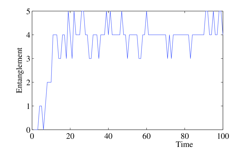
Figure 2: Entanglement evolution of stabilizer states where $N=10$ and $N_{A}=5$. Here a single realization only. The dramatic jumps reflect the fact that stabilizer entanglement only comes in integer values.

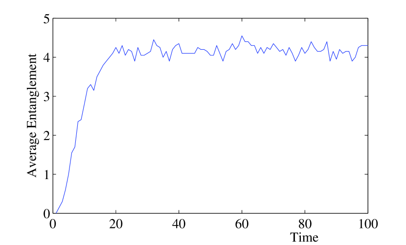
Figure 3: Here averaged over 20 realizations. One sees that the average behaviour is like that of general states.

5 Two phases in approach to typical entanglement

Theorem 1 tells us that systems undergoing this sort of random interactions will tend to become maximally entangled very fast. Numerical studies in addition reveal a finer structure in the approach, namely two phases, apparently separated by a well-defined and short transition interval.

1. A phase in which entanglement is rapidly increasing and spreading through the system.

2. A phase in which entanglement has spread through the entire system.

We identify three ways of defining the moment of time that separates these two phases that will be explained in the following: the saturation moment $\tau_{sat}$, the cutoff moment $\tau_{cutoff}$ or the volume scaling moment $\tau_{vol}$.

5.1 Saturation moment

Applying the random interaction we make the following
Observation: There is a moment of saturation of the average entanglement.

Before this moment the average block entanglement increases essentially linearly in the time $n$. After the transition moment it is however practically constant and nearly maximal. Therefore we term the transition time between the two regimes the ’saturation time’ $\tau_{sat}$. There is some degree of freedom in what exact value to assign to this time. One could for example specify $\tau_{sat}(\epsilon)$ as the moment that the gradient of the average entanglement curve is within some fixed accuracy $\epsilon$ to 1. Figure 4 shows how this moment is reached.

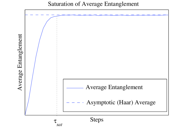
Figure 4: Illustrating $\tau_{sat}$. We find that this behaviour is generic from numerical simulations.

5.2 Cut off moment

The numerical observation that there appears to be two time-scales involved here, first a rapid approach to the asymptotic value and then a slow one, led us to study the statistical mathematics literature for tools that quantify this. In fact there has been extensive study of such problems, motivated by the fact that a randomisation process, such as shuffling cards in a casino, is in practise performed only a finite number of times. The question is then, how many shuffles are necessary before one is certain, for all practical purposes, that the cards are shuffled. In the setting concerned here, that corresponds to asking when we are certain, for practical purposes, that the entanglement probability distribution has achieved its asymptotic form. The tool we will use here is the so called ”cut-off effect”, which is exhibited by many Markov Chains[38].

The cut-off refers to an abrupt approach to the stationary distribution occurring at a certain number of steps taken in the chain. Say we have a Markov chain defined by its transition matrix P, and that it converges to a stationary distribution $\pi$. Initially the total variation distance $TV=\parallel P-\pi\parallel=sup\mid P(E)-\pi(E)\mid$ between the corresponding probability distributions is given by $TV=1$. After $k$ steps this distance is given by $TV(k)=\parallel P^{k}-\pi\parallel$. A cut-off occurs, basically, if $TV(k)\simeq 1$ for $k=0,1,2,...a$ and thereafter falls quickly such that after a few steps $TV(k)\simeq 0$. As we increase the size of the state space, the number of steps during which the abrupt approach takes place should decrease compared to $a$, the number of steps necessary to reach the cut off. Then, for very large state spaces, we can say that the randomisation occurs at $a$ steps, some function of the size of the state space.

As a precise definition of a cut off we use [38].
Definition: Let $P_{n}$, $\pi_{n}$ be Markov Chains on sets $\chi_{n}$. Let $a_{n}$, $b_{n}$ be functions tending to infinity, with $\frac{b_{n}}{a_{n}}$ tending to zero. Say the chains satisfy an $a_{n}$, $b_{n}$ cutoff if for some starting states $x_{n}$ and all fixed real $\theta$ with $k_{n}=\lfloor a_{n}+\theta b_{n}\rfloor$, then

$$\parallel P_{n}^{k_{n}}-\pi_{n}\parallel\longrightarrow c(\theta)$$ (29)

with $c(\theta)$ a function tending to zero for $\theta$ tending to infinity and to 1 for theta tending to minus infinity.

With this definition it is now possible to study whether there is a sharp cut-off time associated with the entanglement probability distribution, a functional on our specific Markov process. Indeed, numerically we make the
Observation: We observe an apparent cut off effect in the entanglement probability distribution under the two-particle interaction random process described in this work.

Figure 5 shows an example of a cut off for general states. The state space has been discretised by rounding off entanglement values to the nearest integer. We observe that $TV\simeq 1$ for a while and then falls. Finally there is a stage where $TV\simeq 0$. The effect becomes more pronounced with increasing $N$.

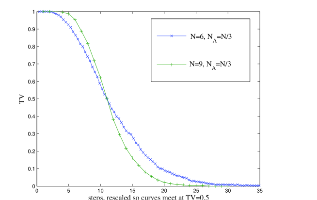
Figure 5: Observe cut-off effect for general states. The total variation distance to the asymptotic entanglement probability distribution, $TV\simeq 1$ for some finite time, before falling to 0. The fall becomes more dramatic with increasing system size. Note that, as is the customary way of representing this effect, we have rescaled the curves to meet where $TV\simeq 0.5$.

Now consider the analogous situation for stabilizer states. From Lemma 4 we would expect this behaviour to be representative of that of general states. Since stabilizer states are efficiently parameterised, using them this will allow us to scale further with N.

Observation: We observe an apparent cut off effect in the entanglement probability distribution under the stabilizer two-particle interaction random process described in this work.

How this squeezes up is showed for individual runs, averaged over 1000 realizations, in figure 6.

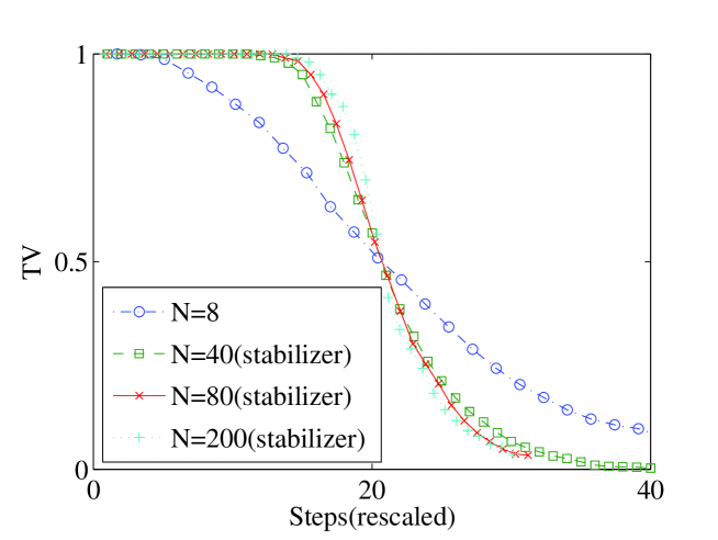
Figure 6: The cut-off effect in the total variation distance ($TV$) is here studied for larger $N$ by employing stabilizer states and tools to efficiently evaluate their entanglement[31]. One sees that the effect becomes increasingly pronounced with increasing $N$. We conjecture that the function is a step function in the limit of $N\rightarrow\infty$, consistent with the normal behaviour of the cut-off effect.

As stated, the cut off effect is common in classical Markov Chains such as card shuffling [38]. It is a testament to the universality of mathematics that applying quantum gates at random to a quantum register apparently exhibits the same features, in this regard, as applying shuffles to a deck of cards.

We term this the cut off moment $\tau_{cutoff}$. Using this moment to separate the first and second phase has the advantages that it unambiguously gives one moment, and this moment corresponds to the point when the entanglement distribution equals, for practical purposes, the asymptotic one.

5.3 The area to volume scaling transition

We now consider the two-party random process restricted to nearest-neighbours interactions, as in figure 7.

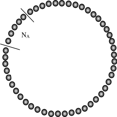
Figure 7: $N$ qubits with nearest neighbour interactions. We vary $N_{A}$ at different times and ask what the typical entanglement is.

This helps us to relate two pictures of typical entanglement. One is the notion that following a randomising process entanglement appears all pervasive in the system. In this case one may expect that the entanglement between two blocks scales roughly as the size of the smaller part, i.e. we observe a volume scaling. While this is the behaviour for generic states it is in strong contrast to the behaviour of pure states that are typically appearing in nature such as the ground states of Hamilton operators describing systems with short range interactions. Indeed, in such systems the block entanglement in ground states has been proven to scale as the boundary surface area between the two blocks for a wide variety of systems [43, 44, 45, 46]. This indicates that ground states of short-range Hamiltonians tend to explore only a tiny fraction of the entire Hilbert space as their entanglement properties are indeed rather atypical.

Numerical Observation: The entanglement scales as the area at small times and as the volume of the smaller block at large times.

This observation motivates the introduction of the transition time from area to volume scaling $\tau_{vol}$ and is shown in figure 8. The result could have been expected since the nearest neighbour structure is only respected at small times since at longer times the two-qubit unitaries have combined to form global unitaries. To assign an exact value to this moment one can specify $\tau_{vol}(\epsilon)$ as the moment $max|\mathbb{E}\left[S(\rho_{A})\right]-\mathbb{E}\left[S(\rho_{A,\tau})\right]|\leq\epsilon$ where the maximisation is over all partitions.

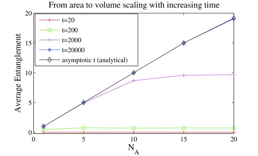
Figure 8: $N=40$ qubits with nearest neighbour interactions. We vary $N_{A}$ at different times and ask what the typical entanglement is. Sufficiently high statistics were taken that the statistical error was not visible on this plot. The asymptotic curve was calculated using equation 28.

6 Multipartite and mixed states

So far we have considered pure bipartite states. It is known that the unitarily invariant measure is not uniquely defined for mixed states however. This can be visualised already in the case of one qubit. On one qubit a unitary time evolution corresponds to a rotation of the Bloch Sphere. Pure states lie on the surface of the sphere and the unitarily invariant measure is an uniform distribution on the surface of the sphere. However mixed states can lie anywhere in the ball inside the sphere and there is no longer a unique measure as unitary invariance does not provide any restrictions on the radial distribution. Mixed measures may be induced by considering environments that allow for purifications of mixed states. Then the measure will be obtained by using the uniform measure on the purifications and then determine the measure that is obtain by partial tracing. Nevertheless some ambiguity remains related to the size of the environment. As is evident from the results here, increasing the size of the environment concentrates the measure more and more around the maximally mixed state.

Before evaluating the entanglement between A and B one traces out the environment C. This leads to AB to be in a mixed state. In fact, with increasing size of the environment the state of AB tends to become more mixed and the entanglement between A and B becomes negligible and ultimately disappears. This is a possible argument for emerging classicality. To measure entanglement in the mixed state we used the logarithmic negativity, $E_{N}$, defined in [47, 48, 49] and proven to be an entanglement monotone in [48].

$$E_{N}(\rho)=log_{2}||\rho^{T_{A}}||_{1}.$$ (30)

Hence here the entanglement is quantified as $E_{N}(tr_{C}(\rho_{ABC}))$ One can also note that for mixed states there are classical correlations. The mutual information, $S(\rho_{A})+S(\rho_{B})-S(\rho_{AB})$, can be interpreted as the combination of classical and quantum correlations [50].

Observation: The mutual information behaves very similarly to the quantum correlations (entanglement)in the two particle-interaction random walk simulations.

This suggest the classical correlations behave similarly to the entanglement in the random two-party process, as in figure 9.

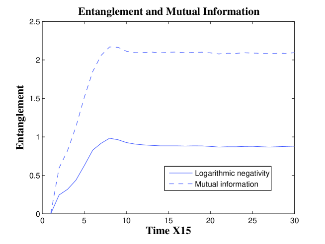
Figure 9: An example of a numerical simulation showing that the average classical and quantum correlations behave similarly. The quantum correlations are quantified using the logarithmic negativity. The combination of classical and quantum correlations is quantified using the mutual information. Here $N=10$, $N_{A}=3$, $N_{B}=3$ and $N_{C}=4$.

The usefulness of the entanglement as a possible macroscopic parameter is highlighted in figure 10 which shows how the equilibrium values is an attractor point regardless of initial state and that there is a flow towards this point. The latter observation hints that the average entanglement is a good parameter also in the approach to the attracting equilibrium.

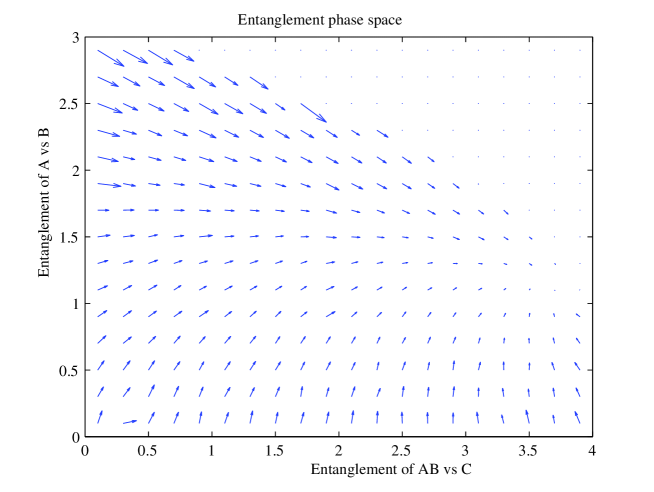
Figure 10: Entanglement ’Phase space’ flow diagram. The arrows point in the average flow direction and the length indicates the speed. The entanglement between A and B is quantified as $E_{N}(tr_{C}(\rho_{ABC}))$ and the entanglement between AB and C using $S(\rho_{C})$ We see how different initial states will all tend to the attractor point. The horizontal coordinate of this point is given by equation 1. The vertical coordinate by $\mathbb{E}\left[E_{N}(tr_{C}(\rho_{ABC}))\right]$. Here $N=10$, $N_{A}=3$, $N_{B}=3$ and $N_{C}=4$. The region in the top right corner is empty as such states are not physically realizable.

6.1 Simplified multipartite description

Considering generic entanglement only will hopefully provide simplifications in various settings. Here we suggest a way in which it simplifies the multipartite setting. We consider the tripartite setting. Let $N$ qubits be shared between three parties of size $N_{A}$, $N_{B}$ and $N_{C}$, s.t. $N_{A}+N_{B}+N_{C}=N$ and $N_{A}\leq N_{B}\leq N_{C}$. We can then consider many types of bipartite cuts. Let $E(A|B)$ signify the (unitarily invariant) entanglement average of the entanglement across the $A|B$ cut after C has been traced out, and let $E(A+B|C)$ signify the corresponding quantity across the $A+B\|C$ cut. The set $\Omega$ of all possible bipartite entanglement averages is then $\Omega=\{E(A|B),E(A|C),E(B|C),E(A+B|C),E(A+C|B),E(B+C|A)\}$. Let these values specify ’the tripartite entanglement’. Now for an arbitrary state, it is not the case that $\Omega$ is uniquely determined by $E(A|B)$ together with $E(A+B|C)$. However we make the following claim.

Conjecture: $\Omega$ is uniquely determined by $E(A|B)$ together with $E(A+B|C)$

Support for conjecture: Firstly note that if $N_{A}$, $N_{B}$ and $N_{C}$ are specified then $\Omega$ is uniquely determined. Then we need the following two statements to be true to prove the claim:

1.$N_{A}+N_{B}$ and $N_{C}$ are uniquely specified by $E(A+B|C)$. This is true if the Von Neumann entropy of entanglement increases monotonically when a qubit is given from the larger of the two parties to the smaller. We are concerned with the limit of large $N$, where equation 1 implies that $N_{C}=\lceil E(A+B|C)\rceil$ assuming $N_{C}\leq N_{A}+N_{B}$

2. For the given $N_{C}$ and $N$, $N_{A}$ and $N_{B}$ are uniquely determined by $E(A|B)$. Again one should be able to use a monotonicity argument here, although it will be more difficult due to the lack of a neat closed form of $E(A|B)=\mathbb{E}\left[E_{N}(tr_{C}(\rho_{ABC}))\right]$. It seems reasonable to expect it to be monotonous though since since $N_{C}$ is fixed.

This idea could presumably be extended to more than three parties and may lead to a description that is highly useful by virtue of requiring very few parameters.

7 Discussion and Conclusion

The entanglement evolution during random two-qubit interactions was studied in some depth and we have provided a detailed proof of the result presented in [1] that the average entanglement approaches the unitarily invariant value within $O(N^{3})$ steps. The essential idea of the proof is a map from the evolution in state space onto one on a much smaller space that tracks the evolution of the purity of the reduced subsystem. We then proved that the process can be simulated efficiently on a classical computer using stabilizer states.

We found through numerical studies that there are two phases in the approach: first a phase during which entanglement is rapidly spreading through the system, and then a phase where the entanglement is suffused throughout the system. Three moments of time that could be used to define the partition between these phases were introduced and discussed. Firstly the saturation of the average $\tau_{sat}$ was considered followed by the cut off moment $\tau_{cutoff}$. Then we noted that if one restricts the interactions to be between nearest neighbours, the entanglement initially scales as the area of the smaller region and in the second phase as that of the volume. This led us to introduce $\tau_{vol}$, the moment the entanglement is typically volume scaling. Of these perhaps the cut off moment $\tau_{cutoff}$ is the most attractive choice, since it gives an unambiguous single time that corresponds to the moment that the entanglement probability distribution is equal to, for practical purposes, that of the unbiased distribution of pure states.

The results support the relevance of generic entanglement as we show it can be generated efficiently from two-qubit gates. Therefore protocols relying on typical/generic entanglement, like [42, 26, 25, 16] gain relevance[1].

The above results may be extended in various directions that will be described briefly here.

Multi-particle entanglement measures – It would be interesting to extend the above results to further investigate properties of typical multi-partite entanglement. For entanglement measures based on average purities [2] this is possible with the results established here. Other measures such as the entanglement of formation may also be treated but require extensions of the approach presented here that go beyond the scope of this paper.

Markov Process Quantum Monte Carlo Methods – Our results possess another interpretation that is of interest for the numerical study of quantum-many-body systems. One numerical approach to classical spin systems is to evolve spin configurations randomly according to the Metropolis rule, i.e. always accepting moves that decrease energy and accepting moves that increase energy with a probability proportional to $exp\{-\Delta E/kT\}$. This reproduces the correct thermal average. One may of course consider a similar approach in the quantum setting applying random two-qubit gates to progress the state. Our present results fall into this category but apply for infinite temperatures as we draw our unitaries from the invariant Haar measure. However, we may adapt our analysis to the finite temperature regime employing stabilizer states at the expense of having to analyze a more complicated Markov process. Basic ideas of our approach carry over and open the possibility for rigorous statements concerning the convergence rate of such a Markov Process Quantum Monte Carlo approach.

Continuous Variables – These question are made additionally complicated in the continuous variable setting through the lack of a Haar measure in the setting of non-compact groups. However in [53] an approach to proceed is introduced. There one notes that it is reasonable to assume that the maximum energy of the global pure state is finite. This tames the non-compactness and one can define a way to pick states at random. Reference [53, 54] gives an explicit method to achieve that for Gaussian states, which probably will take on the role analogous to stabilizer states in the general setting. This opens up the possibility of studying the questions dealt with here in the continuous setting.

Two phases – The relation between the three moments of time that can be used to separate the two phases we observe should be further investigated. We believe analytical tools for studying the cut-off effect are sufficiently developed to undertake an analysis with the aim of proving relations between $\tau_{vol}$, $\tau_{cutoff}$, and $\tau_{sat}$ respectively.

Relation to other work – It would be interesting to investigate how our results relate to existing work on Spin-gases[55] which are similarly semi-quantal systems. We also hope to relate this line of enquiry to work touching on what the typical entanglement of the universe is[57, 56]. The main difference to the approach here would be to consider closed systems.

Experimental studies – Optical lattices appear to provide a suitable experimental setting to test the results obtained here. There is also hope of using Bose-Einstein condensates or linear optics to study the continuous variable case.

Acknowledgements – We gratefully acknowledge initial discussion with Jonathan Oppenheim as well as discussions with Koenraad Audenaert, Fernando Brandao, Benoit Darquie, Jens Eisert, David Gross, Konrad Kieling, Terry Rudolph, Alessio Serafini, Graeme Smith, John Smolin, Andreas Winter, and Aram Harrow.

We acknowledge support by the EPSRC QIP-IRC, The Leverhulme Trust, EU Integrated Project QAP, the Royal Society, the NSA, the ARDA through ARO contract number W911NF-04-C-0098, and the Institute for Mathematical Sciences at Imperial College London.

8 Appendix A: Uniform (Haar) measure on the unitary group

We here briefly introduce the often used uniform measure on pure states, sometimes called the unitarily invariant measure. This is a particular instance of a Haar measure, which can be viewed as a generalization of the ’flat distribution’. A flat probability distribution is the one reflecting no bias with respect to any object.

Such a distribution on a set of objects is invariant under permutations of the said objects. Therefore if there is a group of transformations associated with the set of elements, the distribution on those elements should be invariant under application of elements of the group. The simplest non-trivial example is probably a coin. Here there are two group elements, the identity and the flip. Only the unbiased probability distribution P(Head)=1/2 and P(Tail)=1/2 is invariant under those transformations.

Bearing this in mind, consider picking pure general states at random. The unbiased distribution on pure states is here required to be invariant under unitary transforms, i.e. $P(|\Psi\rangle)=P(U|\Psi\rangle)$, where it is implicit that we are in a continuous setting. This requirement uniquely defines the distribution. For a single qubit this can be nicely visualised as a uniformly dense distribution on the Bloch sphere, see figure 11.

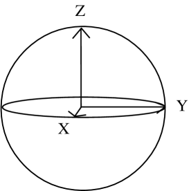
Figure 11: Bloch sphere: the unitarily invariant distribution corresponds to a uniform distribution over this sphere.

The normal method to pick pure states from this distribution is to fix an arbitrary pure state and apply a unitary picked at random from the associated measure on unitary matrices. See for example [52] for the explicit procedure.

9 Appendix B: Randomizing properties of Haar measure

The following lemma shows that Requirement 1 is satisfied by our example with Haar measure.

Lemma 5.

Suppose $F=F(A,B)$ is a bi-linear function of one-qubit operators $A$, $B$, that $\sigma_{a},\sigma_{b}$ are two Pauli matrices, and that $I$ is randomly drawn from Haar measure on $U(2)$. Then

$$\mathbb{E}\left[F(T\sigma_{a}T^{\dagger},T\sigma_{b}T^{\dagger})\right]=\left\{\begin{array}[]{ll}F(I,I),&a=b=0;\\ \frac{1}{3}\sum_{w\in\{x,y,z\}}F(\sigma_{w},\sigma_{w}),&a=b\neq 0\\ 0,&\mbox{otherwise.}\end{array}\right.$$

To prove it, we need an intermediate result.

Lemma 6.

Assume that $\sigma_{a}$, $a\neq 0$, is a Pauli operator and $T$ is a random unitary drawn from Haar measure on $U(2)$. Then

$$T\sigma_{a}T^{\dagger}=r_{x}\sigma_{x}+r_{y}\sigma_{y}+r_{z}\sigma_{z},$$

where $(r_{x},r_{y},r_{z})$ is a random vector whose distribution is invariant under permutations. Moreover, $\mathbb{E}\left[r_{u}r_{u^{\prime}}\right]=\delta_{u,u^{\prime}}/3$ for all $u,u^{\prime}\in\{x,y,z\}$.

Proof.

$T\sigma_{a}T^{\dagger}$ is a $2\times 2$ Hermitian matrix. Therefore, there exist real numbers (in fact random variables) $r_{u}=\Tr(\sigma_{u}T\sigma_{a}T^{\dagger})/2$ ($u\in\{0,x,y,z\}$) such that

$$T\sigma_{w}T^{\dagger}=r_{0}I+r_{x}\sigma_{x}+r_{y}\sigma_{y}+r_{z}\sigma_{z}.$$

$\Tr{(T\sigma_{a}T^{\dagger})}=\Tr(\sigma_{a})=0$ implies $r_{0}=0$. Before we continue, let us state a simple fact we will use repeatedly.

Claim 2 (Conjugation trick).

For any unitary $Q\in U(2)$, $T\sigma_{a}T^{\dagger}$ and $QT\sigma_{a}T^{\dagger}Q^{\dagger}=QT\sigma_{a}(QT)^{\dagger}$ have the same probability distribution. Therefore, the distribution of $(r_{x},r_{y},r_{z})$ is the same as that of $(r^{\prime}_{x},r^{\prime}_{y},r^{\prime}_{z})$, where

$$r^{\prime}_{u}=\frac{1}{2}\,\Tr(\sigma_{u}QT\sigma_{w}T^{\dagger}Q^{\dagger})=\frac{1}{2}\,\Tr((Q\sigma_{u}Q^{\dagger})T\sigma_{w}T^{\dagger}).$$ (31)

In fact, this follows directly from the invariance property of Haar measure. Since $T$ and $QT$ have the same probability distribution, so do $T\sigma_{a}T^{\dagger}$ and $QT\sigma_{a}(QT)^{\dagger}$ (which are the same deterministic function of $Q$ and $QT$, respectively) and the same holds for $(r_{x},r_{y},r_{z})$ is the same as that of $(r^{\prime}_{x},r^{\prime}_{y},r^{\prime}_{z})$.

We now apply the trick as follows.

1. Take $Q=H$ (the Hadamard matrix). Then $Q\sigma_{x}Q^{\dagger}=\sigma_{z}$, $Q\sigma_{z}Q^{\dagger}=\sigma_{x}$ and $Q\sigma_{y}Q^{\dagger}=\sigma_{y}$. This implies that $2r^{\prime}_{x}=Tr((Q\sigma_{x}Q^{\dagger})T\sigma_{a}T^{\dagger})=Tr(\sigma_{y}T\sigma_{w}T^{\dagger})=2r_{y}$, $2r^{\prime}_{y}=Tr((Q\sigma_{y}Q^{\dagger})T\sigma_{a}T^{\dagger})=Tr(\sigma_{z}T\sigma_{a}T^{\dagger})=2r_{x}$ and $r^{\prime}_{z}=r_{z}$. Hence $(r^{\prime}_{x},r^{\prime}_{y},r^{\prime}_{z})=(r_{z},r_{y},r_{x})$ and $(r_{x},r_{y},r_{z})$ have the same distribution.

2. Now take $Q=|\,0\rangle\langle 0\,|-i|\,1\rangle\langle 1\,|$. $Q\sigma_{x}Q^{\dagger}=\sigma_{y}$, $Q\sigma_{y}Q^{\dagger}=\sigma_{x}$ and $Q\sigma_{z}Q^{\dagger}=\sigma_{z}$. It follows from the above reasoning that $(r_{y},r_{x},r_{z})$ and $(r_{x},r_{y},r_{z})$ have the same distribution.

3. Take $Q=\sigma_{z}$ this time. Then $Q\sigma_{x}Q^{\dagger}=-\sigma_{x}$, $Q\sigma_{y}Q^{\dagger}=-\sigma_{y}$, $Q\sigma_{z}Q^{\dagger}=\sigma_{z}$, so $(-r_{x},-r_{y},r_{z})$ and $(r_{x},r_{y},r_{z})$ have the same distribution. Similarly Similarly, we can take $Q=\sigma_{y}$ or $Q=\sigma_{x}$ to show that $(-r_{x},r_{y},-r_{z})$ and $(r_{x},-r_{y},-r_{z})$ also have the same distribution.

The first two items show that the distribution of $(r_{x},r_{y},r_{z})$ is invariant by transposition of the $x$ and $z$ coordinates and of the $x$ and $y$ coordinates. It follows that the distribution is also invariant under transposition of the $y$ and $z$ coordinates (which is a composition of a $xz$ transposition followed by a $xy$ transposition and another $xz$ transposition). Since any permutation is a composition of transpositions, we have shown that the the distribution of $(r_{x},r_{y},r_{z})$ is invariant under permutations of the coordinates. Moreover, it also follows that

$$1=\frac{\Tr(\sigma_{w}^{2})}{2}=\frac{1}{2}\mathbb{E}\left[\Tr[(T\sigma_{w}T^{\dagger})^{2}]\right]=\mathbb{E}\left[r_{x}^{2}+r_{y}^{2}+r_{z}^{2}\right]=3\mathbb{E}\left[r_{u}^{2}\right]\mbox{ for all }u\in\{x,y,z\}.$$

Thus it only remains to show that $\mathbb{E}\left[r_{u}r_{u^{\prime}}\right]=0$ if $u\neq u^{\prime}$. To this end, we use item $3.$ If for instance $u=x$, $u^{\prime}=z$ we recall that $(-r_{x},-r_{y},r_{z})$ and $(r_{x},r_{y},r_{z})$ have the same distribution, hence $r_{x}r_{z}$ and $-r_{x}r_{z}$ also have the same distribution, which implies our claim. The other cases follow similarly.∎

We can now prove Lemma 5.

Proof.

First assume that $a\neq b$. Without loss of generality, assume that $b\neq 0$. We apply an idea based on the Conjugation Trick from the previous proof. There exists $c\in\{x,y,z\}$ such that $\sigma_{a}$ and $\sigma_{c}$ commute and $\sigma_{b}$ anti-commutes with $\sigma_{c}$. As $U$ and $U\sigma_{c}$ have the same distribution, $(U\sigma_{c})\sigma_{a}(U\sigma_{c})^{\dagger}=U\sigma_{a}U^{\dagger}$ and $(U\sigma_{c})\sigma_{b}(U\sigma_{c})^{\dagger}=-U\sigma_{b}U^{\dagger}$, we have

$$\mathbb{E}\left[F(U\sigma_{a}U^{\dagger},U\sigma_{b}U^{\dagger})\right] = \mathbb{E}\left[F((U\sigma_{c})\sigma_{a}(U\sigma_{c})^{\dagger},(U\sigma_{c})\sigma_{b}(U\sigma_{c})^{\dagger})\right]$$

$$= -\mathbb{E}\left[F(U\sigma_{a}U^{\dagger},U\sigma_{b}U^{\dagger})\right],$$

thus the expected value is $0$. Now if $a=b=0$, the result is trivial. If $a=b\neq 0$, we can write $U\sigma_{a}U^{\dagger}=r_{x}\sigma_{x}+r_{y}\sigma_{y}+r_{z}\sigma_{z}$ as in Lemma 6, and by bi-linearity

$$\mathbb{E}\left[F(U\sigma_{a}U^{\dagger},U\sigma_{a}U^{\dagger})\right]=\sum_{w^{\prime},w^{\prime\prime}}\mathbb{E}\left[r_{w^{\prime}}r_{w^{\prime\prime}}\right]F(\sigma_{w^{\prime}},\sigma_{w^{\prime\prime}}).$$ (32)

Applying Lemma 6 finishes the proof.∎

10 Appendix C: Stabilizer states

Stabilizer states are a discrete subset of general quantum states, which can be described by a number of parameters scaling polynomially with the number of qubits in the state [28, 29, 8].

A stabilizer operator on $N$ qubits is a tensor product of operators taken from the set of Pauli operators

$$\sigma_{1}:=\left(\begin{array}[]{cc}0&1\\ 1&0\end{array}\right),\,\,\sigma_{2}:=\left(\begin{array}[]{cc}0&-i\\ i&0\end{array}\right),\,\,\sigma_{3}:=\left(\begin{array}[]{cc}1&0\\ 0&-1\end{array}\right),$$ (33)

and the identity $I$. An example for $N=3$ would be the operator $g=\sigma_{1}\otimes I\otimes sigma_{3}$. A set $G=\{g_{1},\ldots,g_{K}\}$ of $K$ mutually commuting stabiliser operators that are independent, i.e. $\prod_{i=1}^{K}g_{i}^{s_{i}}=I$ exactly if all $s_{i}$ are even, is called a generator set. For $K=N$ a generator set $G$ uniquely determines a single state $|\psi\rangle$ that satisfies $g_{k}|\psi\rangle=|\psi\rangle$ for all $k=1,\ldots,N$. Such a generating set generates the stabilizer group. Each unique such group in turn defines a unique stabilizer state.

For example the GHZ state $|000\rangle+|111\rangle$ is defined by the generator set $\langle\sigma_{1}\otimes\sigma_{1}\otimes\sigma_{1},\sigma_{0}\otimes\sigma_{3}\otimes\sigma_{3},\sigma_{3}\otimes\sigma_{3}\otimes\sigma_{0}\rangle$.

A key observation that is useful for the considerations here is the fact that the bipartite entanglement of a stabilizer state, i.e. the entanglement across any bipartite split, takes only integer values [31, 32].

Finally we note the fact that in order for the stabilizer state to be non-trivial it is necessary and sufficient that the elements of the stabilizer group (a) commute, and (b) are not equal to -I [8].

References

- [1] R. Oliveira, O.C.O. Dahlsten and M.B. Plenio, Efficient Generation of Generic Entanglement, E-print arXiv:quant-ph/0605126 (To appear in Phys. Rev. Lett.).
- [2] M.B. Plenio and S. Virmani, An introduction to entanglement measures, Quant. Inf. Comp. 7, 1 (2007) and E-print arXiv:quant-ph/0504163.
- [3] M. Horodecki (2001), Entanglement measures, Quant. Inf. Comp. 1,1 (pp3-26).
- [4] W. Wootters (2001), Entanglement of formation and concurrence, Quant. Inf. Comp. 1,1 (pp27-44).
- [5] P. Horodecki, R. Horodecki (2001), Distillation and bound entanglement, Quant. Inf. Comp. 1,1 (pp45-75).
- [6] M.B. Plenio and V. Vedral, Entanglement in Quantum Information Theory, Contemp. Phys. 39, 431 (1998).
- [7] J. Eisert and M.B. PlenioIntroduction to the basics of entanglement theory of continuous-variable systems, Int. J. Quant. Inf. 1, 479 (2003).
- [8] M. Nielsen and I. Chuang, Quantum Information and Computation, Cambridge University Press.
- [9] J. Eisert and D. Gross, E-print arXiv:quant-ph/0505149.
- [10] C. H. Bennett, S. Popescu, D. Rohrlich, J. A. Smolin and A. V. Thapliyal, Exact and Asymptotic Measures of Multipartite Pure State Entanglement, Phys. Rev. A. 63, 012307 (2001).
- [11] N. Linden, S. Popescu, B. Schumacher and M. Westmoreland, Reversibility of local transformations of multiparticle entanglement, E-print arXiv:quant-ph/9912039.
- [12] E. Galvão, M.B. Plenio and S. Virmani, Tripartite entanglement and quantum relative entropy, J. Phys. A 33, 8809 (2000).
- [13] S. Wu and Y. Zhang, Multipartite pure-state entanglement and the generalized Greenberger-Horne-Zeilinger states, Phys. Rev. A 63, 012308 (2001).
- [14] S. Ishizaka, Bound Entanglement Provides Convertibility of Pure Entangled States , Phys. Rev. Lett. 93, 190501 (2004).
- [15] S. Ishizaka and M.B. Plenio, Multiparticle entanglement manipulation under positive partial transpose preserving operations , Phys. Rev. A 71, 052303 (2005).
- [16] P. Hayden, D.W. Leung and A. Winter, Aspects of generic entanglement. , Comm. Math. Phys. 265, 95 (2006).
- [17] E.Lubkin (1978), Entropy of an n-system from its correlation with a k-reservoir, J. Math. Phys 19(5).
- [18] S.Lloyd and H.Pagels (1988), Complexity as Thermodynamic Depth., Ann. of Phys. 188, 186-213.
- [19] D.N.Page (1993), Average entropy of a subsystem, Phys. Rev. Lett. 71 No.9, (1993).
- [20] S.K Foong and S.Kanno (1994), Proof of Page’s conjecture on the average entropy of a subsystem, Phys. Rev. Lett. 72 No. 8.
- [21] J.Emerson, E.Livine, S.Lloyd Random Circuits and Pseudo-Random Unitary operators for Quantum Information Processing, Science 302: 2098Ch-2100, 2003.
- [22] J.Emerson, E.Livine, S.Lloyd. Convergence conditions for random quantum circuits, Phys. Rev. A 72, 060302 (2005).
- [23] J. Emerson, Random Circuits and Pseudo-Random Unitary Operators for Quantum Information Processing, QCMC04, AIP Conf. Proc. 734, 139 (2004).
- [24] G.Smith, D.W.Leung, Typical Entanglement of Stabilizer States, E-print arXiv:quant-ph/0510232.
- [25] H. Buhrman, M. Christandl, P. Hayden, H.K. Lo, and S. Wehner. On the (im)possibility of quantum string commitment, E-print arXiv:quant-ph/0504078.
- [26] A. Harrow, P. Hayden, and D. Leung. Superdense coding of quantum states, Phys. Rev. Lett., 92:187901, 2004.
- [27] D. P. DiVincenzo, D. W. Leung, and B. M. Terhal, Quantum data hiding IEEE Trans. Inf. Theory, 48(3):580 598, 2002.
- [28] D. Gottesman, Stabilizer Codes and Quantum Error Correction, Caltech PhD thesis.
- [29] D. Gottesman (1998), The Heisenberg Representation of Quantum Computers, E-print arXiv:quant-ph/9807006.
- [30] O.C.O.Dahlsten and M.B.Plenio, Entanglement probability distribution of bi-partite randomised stabilizer states, Quant. Inf. Comp. 6, 527-538, (2006).
- [31] K.M.R. Audenaert and M.B. Plenio (2005), Entanglement on mixed stabilizer states: normal forms and reduction procedures, New J. Phys. 7, 170. Note that the Matlab codes in this work can be downloaded from www.imperial.ac.uk/quantuminformation.
- [32] D. Fattal, T. S. Cubitt, Y. Yamamoto, S. Bravyi and I.L. Chuang (2004), Entanglement in the stabilizer formalism, E-print:arXiv quant-ph/0406168.
- [33] M. Hein, J. Eisert and H.J. Briegel (2004), Multiparty Entanglement in Graph States, Phys. Rev. A 69, 062311.
- [34] S. Anders, M. B. Plenio, W. Dür, F. Verstraete and H.-J. Briegel, Ground state approximation for strongly interacting systems in arbitrary dimension, Phys. Rev. Lett. 97, 107206 (2006).
- [35] C.Dankert, R.Cleve, J.Emerson, E.Livine, Exact and Approximate Unitary 2-Designs: Constructions and Applications , E-print arXiv:quant-ph/0606161.
- [36] D. Gross, K. Audenaert and J.Eisert, Evenly distributed unitaries: on the structure of unitary designs, E-print arXiv: quant-ph/0611002.
- [37] J. Emerson, R. Alicki, K. Zyczkowski, Scalable Noise Estimation with Random Unitary Operators, J. Opt. B: Quantum Semiclass. Opt. 7, S347, (2005).
- [38] P.Diaconis, The cutoff phenomenon in finite Markov chains, Proc. Natl. Acad. Sci. USA 93, 1659-1664, (1996).
- [39] P.Diaconis, Group Representations in Probability and Statistics, Institute of Mathematical Statistics. Lecture Notes Monograph Series, 11.
- [40] R. Montenegro, P. Tetali, Mathematical Aspects of Mixing Times in Markov Chains. In series Foundations and Trends in Theoretical Computer Science (ed: M. Sudan), volume 1:3, NOW Publishers, Boston-Delft, June 2006. http://www.ravimontenegro.com/research/TCS008-journal.pdf.
- [41] D. J. Aldous and J. Fill, Reversible Markov Chains and Random Walks on Graphs, (book to appear); URL for draft at http://statwww. berkeley.edu/users/aldous/RWG/book.html.
- [42] A.Abeyesinghe, P.Hayden, G.Smith, Optimal Superdense Coding of entangled states, IEEE Trans. Inform. Theory, vol. 52, no. 8, pp. 3635-3641, 2006.
- [43] K. Audenaert, J. Eisert, M.B. Plenio and R.F. Werner, Entanglement Properties of the Harmonic Chain, Phys. Rev. A 66, 042327 (2002).
- [44] M.B. Plenio, J. Eisert, J. Dreissig and M. Cramer, Entropy, entanglement, and area: analytical results for harmonic lattice systems, Phys. Rev. Lett. 94, 060503 (2005)
- [45] M. Cramer, J. Eisert, M.B. Plenio and J. Dreissig, An entanglement-area law for general bosonic harmonic lattice systems, Phys. Rev. A 73, 012309 (2006).
- [46] J. P. Keating, F. Mezzadri, Random Matrix Theory and Entanglement in Quantum Spin Chains, Commun. Math. Phys., Vol. 252, 543-579 (2004).
- [47] G.Vidal and R.F.Werner, A computable measure of entanglement, Phys. Rev. A 65, 32314 (2002).
- [48] M.B.Plenio, Logarithmic Negativity: A Full Entanglement Monotone That is not Convex, Phys. Rev. Lett. 95 090503 (2005).
- [49] J. Eisert, PhD Thesis Universität Potsdam 2001.
- [50] B.Groisman, S.Popescu and A.Winter, On the quantum, classical and total amount of correlations in a quantum state, Phys. Rev. A, vol 72, 032317 (2005).
- [51] CNOT: and is linear.
- [52] P.Diaconis, What is a random matrix, Notices of the AMS, 52, 11, (2005).
- [53] A.Serafini, O.C.O.Dahlsten and M.B.Plenio, Thermodynamical state space measure and typical entanglement of pure Gaussian states, E-print arXiv:quant-ph/0610090.
- [54] A.Serafini, O.C.O.Dahlsten, D.Gross and M.B.Plenio, Canonical and micro-canonical typical entanglement of continuous variable systems , E-print arXiv:quant-ph/0701051.
- [55] J. Calsamiglia, L. Hartmann, W. Dür, and H.-J. Briegel, Entanglement and decoherence in spin gases, Phys. Rev. Lett. 95, 180502 (2005).
- [56] J. Gemmer, A. Otte, and G. Mahler, Quantum Approach to a Derivation of the Second Law of Thermodynamics , Phys. Rev. Lett. 86, 1927, (2001).
- [57] S. Popescu, A.Short, and A. Winter, The foundations of statistical mechanics from entanglement: Individual states vs. averages, Nature Physics 2, 754, (2006).