Quantum reconstruction of an intense polarization squeezed optical state

Abstract

We perform a reconstruction of the polarization sector of the density matrix of an intense polarization squeezed beam starting from a complete set of Stokes measurements. By using an appropriate quasidistribution, we map this onto the Poincaré space providing a full quantum mechanical characterization of the measured polarization state.

Efficient methods of quantum-state reconstruction are of the greatest relevance for quantum optics. Indeed, they are invaluable for verifying and retrieving information. Since the first theoretical proposals firsttheory and the pioneer experiments determining the quantum state of a light field firstexp , this discipline has witnessed significant growth Jarda . Laboratory demonstrations of state tomography are numerous and span a broad range of physical systems, including molecules DWM1995 , ions LMK1996 , atoms KPM1997 , spins spin , and entangled photon pairs WJE1999 .

Any reliable quantum tomographical scheme requires three key ingredients HMR2006 : the availability of a tomographically complete measurement, a suitable representation of the quantum state, and a robust algorithm to invert the experimental data. Whenever these conditions are not met, the reconstruction becomes difficult, if not impossible. This is the case for the polarization of light, despite the fact that many recent experiments in quantum optics have been performed using polarization states. The origin of these problems can be traced back to the fact that the characterization of the polarization state in terms of the total density operator is superfluous because it contains not only polarization information. This redundancy can be easily handled for low number of photons, but becomes a significant hurdle for highly excited states. An adequate solution has been found only recently: it suffices to reconstruct only of a subset of the density matrix. This subset has been termed the “polarization sector” RMF2000 (or the polarization density operator Kar2005 ) since its knowledge allows for a complete characterization of the polarization state KM2004 .

The purpose of this Letter is to report on the first theoretical and experimental reconstruction of intense polarization states. Specifically, we focus on the case of intense squeezed states to confirm how, even in this bright limit, they still preserve fingerprints of very strong nonclassical behavior.

We begin by briefly recalling some background material. We assume a two-mode field that is fully described by two complex amplitude operators, denoted by $\hat{a}_{H}$ and $\hat{a}_{V}$, where the subscripts $H$ and $V$ indicate horizontally and vertically polarized modes, respectively. The commutation relations of these operators are standard: $[\hat{a}_{j},\hat{a}_{k}^{\dagger}]=\delta_{jk}$, with $j,k\in\{H,V\}$. The description of the polarization structure is greatly simplified if we use the Schwinger representation

$$\hat{J}_{1}=\frac{1}{2}(\hat{a}^{\dagger}_{H}\hat{a}_{V}+\hat{a}^{\dagger}_{V}\hat{a}_{H})\,,\qquad\hat{J}_{2}=\frac{i}{2}(\hat{a}_{H}\hat{a}^{\dagger}_{V}-\hat{a}^{\dagger}_{H}\hat{a}_{V})\,,$$

$$\hat{J}_{3}=\frac{1}{2}(\hat{a}^{\dagger}_{H}\hat{a}_{H}-\hat{a}^{\dagger}_{V}\hat{a}_{V})\,,$$ (1)

together with the total photon number $\hat{N}=\hat{a}^{\dagger}_{H}\hat{a}_{H}+\hat{a}^{\dagger}_{V}\hat{a}_{V}$. These operators coincide, up to a factor 1/2, with the Stokes operators, whose average values are precisely the classical Stokes parameters. One immediately finds that $\hat{\mathbf{J}}=(\hat{J}_{1},\hat{J}_{2},\hat{J}_{3})$ satisfies the commutation relations distinctive of the su(2) algebra: $[\hat{J}_{1},\hat{J_{2}}]=i\hat{J}_{3},$ and cyclic permutations. This noncommutability precludes the simultaneous precise measurement of the physical quantities they represent.

The Hilbert space $\mathcal{H}$ describing the polarization structure of these fields has a convenient orthonormal basis in the form of the Fock states for both polarization modes, namely $|n_{H},n_{V}\rangle$. However, it is advantageous to use the basis $|J,m\rangle$ of common eigenstates of $\hat{J}^{2}$ and $\hat{J}_{3}$. Since $J=N/2$, this can be accomplished just by relabeling the Fock basis as $|J,m\rangle\equiv|n_{H}=J+m,n_{V}=J-m\rangle$. Here, for fixed $J$ (i.e., fixed $N$), $m$ runs from $-J$ to $J$ and these states span a $(2J+1)$-dimensional subspace wherein $\hat{\mathbf{J}}$ acts in the standard way. Since any polarization observable has a block-diagonal form in this basis, it seems appropriate to define the polarization density operator as

$$\hat{\varrho}=\bigoplus_{J=0}^{\infty}\hat{\varrho}_{J}=\sum_{J=0}^{\infty}\ \sum_{m,m^{\prime}=-J}^{J}\varrho^{J}_{mm^{\prime}}\ |J,m\rangle\langle J,m^{\prime}|\,.$$ (2)

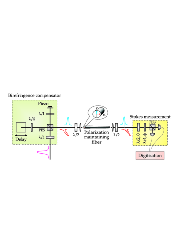
Figure 1: (Color online) Setup for efficient polarization squeezing generation and the corresponding Stokes measurement apparatus.

For a reconstruction of the quantum state one first has to extract the required data from the tomographical measurements. The overall scheme of our experimental setup is illustrated in Fig. 1. The field to be characterized is analyzed using a general polarization measurement apparatus consisting of a half-wave plate $(\lambda/2,\theta)$ followed by a quarter-wave plate ($\lambda/4,\phi$) and a polarizing beam splitter (PBS). The wave plates transform the input polarization allowing the measurement of different Stokes parameters by the projection onto the PBS basis $|J,m\rangle$. The PBS outputs are measured directly using detectors with custom-made InGaAs photodiodes (98% quantum efficiency at DC) and a low-pass filter ($\leq$ 40 MHz) to avoid AC saturation due to the laser repetition rate. The RF currents of the photodetectors were mixed with an electronic local oscillator at 17.5 MHz and digitized with an analog/digital converter at $10^{7}$ samples per second with a 16 bit resolution and 10 times oversampling. The quantum state we measure is defined by the resolution bandwidth of 1 MHz at the 17.5 MHz sideband relative to the 200 THz carrier. Ten digitized sample corresponds to the photocurrent at this sideband generated by photons impinging on the photodiode for 1 $\mu$s. This photodetection can be modelled by the positive operator-valued measure (POVM) agliati05

$$\hat{\Pi}_{m}^{J}=|J,m\rangle\langle J,m|\,,$$ (3)

so that $w_{m}^{J}=\mathop{\mathrm{Tr}}\nolimits(\hat{\varrho}\hat{\Pi}_{m}^{J})$ is the probability of detecting $n_{H}=J+m$ photons in the horizontal mode and simultaneously $n_{V}=J-m$ photons in the vertical one. When the total number of photons $2J$ is not measured and only the difference $2m$ is observed, the POVM is

$$\hat{\Pi}_{m}=\sum_{J=|m|}^{\infty}|J,m\rangle\langle J,m|\,.$$ (4)

The wave plates in the measurement perform linear polarization transformations. These can be described in terms of $\hat{J}_{2}$, which generates rotations about the direction of propagation, and $\hat{J}_{3}$, which generates phase shifts between the modes. In other words, their action is represented by $\hat{\mathcal{R}}(\mathbf{n})=e^{i\theta\hat{J}_{2}}\,e^{i\phi\hat{J}_{3}}$, where $\mathbf{n}=(\cos\phi\sin\theta,\sin\phi\sin\theta,\cos\theta)$ is a unit vector given by the spherical angles $(\theta,\phi)$. The experimental histograms recorded for each $\mathbf{n}$ then correspond to the tomographic probabilities

$$w^{J}_{m}(\mathbf{n})=\mathop{\mathrm{Tr}}\nolimits[\hat{\varrho}\,\hat{\Pi}_{m}^{J}(\mathbf{n})]={}_{\mathbf{n}}\!\langle J,m|\hat{\varrho}|J,m\rangle_{\mathbf{n}}\,,$$ (5)

where $\hat{\Pi}_{m}^{J}(\mathbf{n})=\hat{\mathcal{R}}(\mathbf{n})\,\hat{\Pi}_{m}^{J}\,\hat{\mathcal{R}}^{\dagger}(\mathbf{n})$ and $|J,m\rangle_{\mathbf{n}}$ is the eigenstate of $\mathbf{n}\cdot\hat{\mathbf{J}}$ relative to the eigenvalue $m$, which is precisely a SU(2) coherent state Per1986 . The final tomogram reads

$$w_{m}(\mathbf{n})=\mathop{\mathrm{Tr}}\nolimits[\hat{\varrho}\ \hat{\Pi}_{m}(\mathbf{n})]=\sum_{J=|m|}^{\infty}\ {}_{\mathbf{n}}\!\langle J,m|\hat{\varrho}|J,m\rangle_{\mathbf{n}}\,.$$ (6)

The reconstruction in each $(2J+1)$-dimensional invariant subspace can be now carried out exactly since it is essentially equivalent to a spin $J$ spintom . In fact, after some calculations one finds that the tomograms can be represented in the following compact form

$$w^{J}_{m}(\mathbf{n})=\frac{1}{2\pi}\int_{0}^{2\pi}d\omega\ \mathop{\mathrm{Tr}}\nolimits\left(\hat{\varrho}_{J}\ e^{i\omega\,\mathbf{n}\cdot\hat{\mathbf{J}}}\right)\,e^{-im\omega}\,,$$ (7)

which is precisely the Fourier transform of the characteristic function of the observable $\mathbf{n}\cdot\hat{\mathbf{J}}$.

Inverting this expression, one obtains

$$\hat{\varrho}_{J} = \frac{2J+1}{4\pi^{2}}\int_{0}^{2\pi}d\omega\ \sin^{2}\left(\frac{\omega}{2}\right)$$ (8)

$$\times \int_{\mathcal{S}_{2}}d\mathbf{n}\ e^{-i\omega\,\mathbf{n}\cdot\hat{\mathbf{J}}}\sum_{m=-J}^{J}w_{m}^{J}(\mathbf{n})\,e^{im\omega}\,,$$

where the integration over the solid angle $d\mathbf{n}=\sin\theta\,d\theta d\phi$ extends over the unit sphere $\mathcal{S}_{2}$. By summing over all the invariant subspaces $J$, the density matrix can be reconstructed as follows

$$\hat{\varrho}=\sum_{m=-\infty}^{\infty}\int_{\mathcal{S}_{2}}d\mathbf{n}\ w_{m}(\mathbf{n})\,\mathcal{K}(m-\mathbf{n}\cdot\hat{\mathbf{J}})\,,$$ (9)

where the kernel $\mathcal{K}(x)$ is

$$\mathcal{K}(x)=\frac{2J+1}{4\pi^{2}}\int_{0}^{2\pi}d\omega\ \sin^{2}\left(\frac{\omega}{2}\right)\,e^{-i\omega x}\,.$$ (10)

We stress the appealing analogy of Eq. (9) with the more widely known formula for the reconstruction of the density matrix of a single-mode radiation field from the homodyne tomograms of the rotated quadratures Jarda .

From the exact solution (9), one can calculate any polarization quasidistribution WSU2 . From a computational point of view reconstructing the SU(2) $Q$ function turns out to be the simplest, since in each invariant subspace it reduces to

$$Q(J,\mathbf{n})={}_{\mathbf{n}}\!\langle J,m|\hat{\varrho}|J,m\rangle_{\mathbf{n}}\,,$$ (11)

so, in view of the form (5), it is especially suited for our purposes. The evaluation of the Wigner function can also be carried out, although with additional effort. Nevertheless, we do not expect these two quasidistributions to differ notably for the states we study here. As a consequence, we only need to evaluate the matrix elements of the kernel $\mathcal{K}(m-\mathbf{n}^{\prime}\cdot\hat{\mathbf{J}})$. This can be accomplished using several equivalent techniques, although the most direct way to proceed is to note that

$$\displaystyle{}_{\mathbf{n}}\!\langle J,m|\mathcal{K}(m-\mathbf{n}^{\prime}\cdot\hat{\mathbf{J}})|J,m\rangle_{\mathbf{n}}=\frac{2J+1}{4\pi^{2}}\int_{0}^{2\pi}d\omega\ \sin^{2}\left(\frac{\omega}{2}\right)$$

$$\displaystyle\times\ e^{im\omega}\left[\cos\left(\frac{\omega}{2}\right)-i\sin\left(\frac{\omega}{2}\right)\cos\chi\right]^{2J}\,,$$ (12)

where $\cos\chi=\mathbf{n}\cdot\mathbf{n}^{\prime}$. In the limit of $J\gg~{}1$ the integral in (Quantum reconstruction of an intense polarization squeezed optical state) reduces to $d^{2}\delta(x)/dx^{2}$ evaluated at $x=m-J\,\mathbf{n}\cdot\mathbf{n}^{\prime}$. Since $m$ can be taken as a quasicontinuous variable, we can integrate by parts

$$Q(J,\mathbf{n})=\frac{2J+1}{4\pi^{2}}\int_{-\infty}^{\infty}\!dm\int_{\mathcal{S}_{2}}\!d\mathbf{n}^{\prime}\,\frac{d^{2}w_{m}(\mathbf{n})}{dm^{2}}\,\delta(m-J\,\mathbf{n}\cdot\mathbf{n}^{\prime})\,.$$ (13)

Thus, in the limit of high photon numbers the reconstruction turns out to be equivalent to an inverse 3D Radon transform Dea1983 of the measured tomograms, which greatly simplifies the numerical evaluation of $Q(J,\mathbf{n})$.

To test this theory, we prepared polarization squeezed states by exploiting the Kerr nonlinearity experienced by ultrashort laser pulses in optical fibers heersink05 . Our experimental setup shown in Fig. 1 uses a Cr⁴⁺:YAG laser emitting 140 fs FWHM pulses at 1497 nm with a repetition rate of 163 MHz. Using the two polarization axes of a 13.2 m birefringent fiber (3M FS-PM-7811, 5.6 $\mu$m mode-field diameter), two quadrature squeezed states are simultaneously and independently generated. The emerging pulses’ intensities are set to be identical and they are aligned to temporally overlap. The fiber’s polarization axes exhibit a strong birefringence (beat length 1.67 mm) that must be compensated. To minimize post-fiber losses, we precompensate the pulses in an unbalanced Michelson-like interferometer that introduces a tunable delay between the polarizations heersink03 . A small part (0.1 %) of the fiber output serves as the input to a control loop to maintain a $\pi/2$ relative phase between the exiting pulses, producing a circularly polarized beam.

Since the Kerr effect is photon-number conserving, the amplitude fluctuations of the two individual modes $H$ and $V$ are at the shot-noise level. This was checked using a coherent beam from the laser and employing balanced detection. The average output power from the fiber was 13 mW which, with the bandwidth definition of our quantum state, corresponds to an average number of photons of $10^{11}$ per 1 $\mu$s. The Kerr effect in fused silica generates squeezing up to some Terahertz, making the choice of the sideband in principle arbitrary. The wave plates in the measurement apparatus were rotated by motorized stages. These scanned one quarter of the Poincaré sphere in 64 steps for $\phi$ ($0^{\circ}-22.5^{\circ}$) and 65 steps for $\theta$ ($0^{\circ}-45^{\circ}$), a measurement of which took over 5 hours. The rest of the data can be deduced from symmetry. For each pair of angles, the photocurrent noise of both detectors after the PBS was simultaneously sampled $2.9\times 10^{6}$ times. Noise statistics of the difference of the two detectors’ photocurrents were acquired in histograms with 2048 bins, resulting in the tomograms $w_{m}(\mathbf{n})$. The optical intensity incident on both detectors was recorded as well.

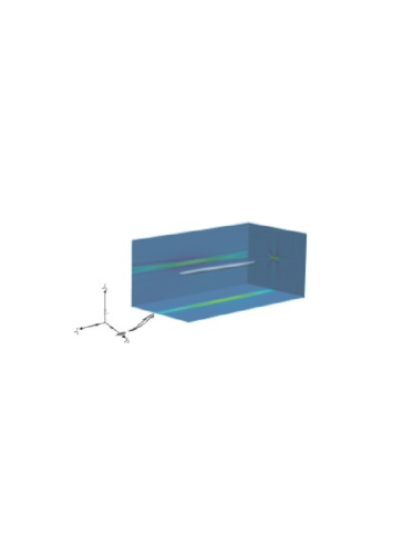
Figure 2: (Color online) Three-dimensional isocontour surface plot of the measured $Q(J,\mathbf{n})$ function for a polarization squeezed state. In the inset, we show the projections over the coordinate planes passing through the origin of the ellipsoid. The projection on the $J_{1}$-$J_{3}$ plane shows typical artifacts from the Radon transform.

To reconstruct the $Q$ function we performed a 3D inverse Radon transform. In Fig. 2 we show the result of the reconstruction for a polarization squeezed state. Here an isocontour surface of the 3D space (or Poincaré space) of $Q(J,\mathbf{n})$ is seen, as well as the projections of this surface. The ellipsoidal shape of the polarization squeezed state is clearly visible. The antisqueezed direction of the ellipsoid is dominated by excess noise stemming largely from Guided Acoustic Brillouin Scattering (GAWBS), which is characteristic for squeezed states generated in optical fibers. Note that this reconstruction of an intense Kerr squeezed state is very hard with conventional homodyne detection techniques for quadrature variables due to the high intensities. The projection of the ellipsoid on the plane $J_{2}$-$J_{3}$ results in an ellipse (and not a circle) because of imperfect polarization contrast in the measurement setup. As the classical excitation of the state is in the $J_{2}$ direction, one expects to reach the shot-noise limit in this projection. After the interference at the PBS all intensity impinges on only one detector. However, with limited polarization contrast some parts of the $>$ 25 dB excess noise from the dark output port can be mixed into the intense beam. Acting as a homodyne measurement this will be visible in the noise of the detector.

In Fig. 3 we compare the isocontour surface plots of a coherent and a polarization squeezed state for the value corresponding to half width at half maximum. The size of the contours agree with the 6.2 $\pm$ 0.3 dB squeezing that was directly measured with a spectrum analyzer.

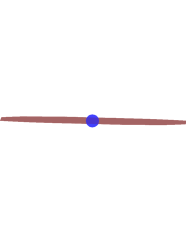
Figure 3: (Color online) Meridional sections of the isocontour surface plots of the $Q$ function for a coherent state (blue) and a polarization squeezed state (red).

By summing over all the values of $J$, we can obtain the total $Q(\mathbf{n})$, which is a probability distribution over the Poincaré unit sphere and is properly normalized. In Fig. 4 we have plotted such a function for the squeezed state. As the state has a large excitation of the order of $10^{11}$ photons and the angles of the distribution on the unit sphere are small, the spherical coordinates can be treated like Cartesian coordinates in the vicinity of the classical point and we present a zoomed version of the surface of the sphere. Again the excess phase noise of the squeezed state is visible. The oscillations with negativities near the main peak are characteristic of artifacts arising from the inverse Radon transformation. These artifacts are more visible for sharp or elongated structures. To improve the reconstruction one would have to go to more sophisticated reconstructions, e.g., maximum likelihood methods Jarda .

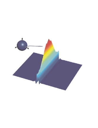
Figure 4: (Color online) Probability distribution over the Poincaré unit sphere for a polarization squeezed state obtained over all invariant subspaces. The distribution is strongly concentrated at the classical mean value, so we show a zoomed version.

In summary, we have presented an exact inversion formula for quantum polarization states and derived a simplified version for high-intensity states. The reconstruction of an intense polarization squeezed state, formed by the Kerr effect in an optical fiber, was performed. Interesting future investigations include the comparison with the maximum likelihood method and the reconstruction of nonclassical polarization states with lower intensity.

We thank V. P. Karassiov for useful discussions and C. Müller for technical assistance. Financial support from the EU (COVAQIAL No FP6-511004), CONACyT (Grant 45704), and DGI (Grant FIS2005-0671) is gratefully acknowledged. M. V. Ch. was supported by DFG (Grants 436 RUS 17-75-05 and 436 RUS 17-76-06).

References

- (1) R. G. Newton and B. L. Young, Ann. Phys. (N. Y.) 49, 393 (1968); W. Band and J. L. Park, Found. Phys. 1, 133 (1970); J. Bertrand and P. Bertrand, ibid 17, 397 (1987); K. Vogel and H. Risken, Phys. Rev. A 40, 2847 (1989).
- (2) D. T. Smithey, M. Beck, M. G. Raymer, and A. Faridani, Phys. Rev. Lett. 70, 1244 (1993).
- (3) U. Leonhardt, Measuring the Quantum State of Light (Cambridge U. Press, Cambridge, 1997); G. M. D’ Ariano, M. G. A. Paris, and M. F. Sacchi, Adv. Imag. Elect. Phys. 128, 205 (2003); Quantum State Estimation, edited by M. G. A. Paris and J. Řeháček, Lect. Not. Phys. Vol. 649 (Springer, Heidelberg, 2004); A. I. Lvovsky and M. G. Raymer, quant-ph/0511044 .
- (4) T. J. Dunn, I. A. Walmsley, and S. Mukamel, Phys. Rev. Lett. 74, 884 (1995).
- (5) D. Leibfried, D. M. Meekhof, B. E. King, C. Monroe, W. M. Itano, and D. J. Wineland, Phys. Rev. Lett. 77, 4281 (1996).
- (6) C. Kurtsiefer, T. Pfau, and J. Mlynek, Nature (London) 386, 150 (1997).
- (7) I. L. Chuang, N. Gershenfeld, and M. Kubinec, Phys. Rev. Lett. 80, 3408 (1998); G. Klose, G. Smith, and P. S. Jessen, ibid 86, 4721 (2001).
- (8) A. G. White, D. F. V. James, P. H. Eberhard, and P. G. Kwiat, Phys. Rev. Lett. 83, 3103 (1999); M. W. Mitchell, C. W. Ellenor, S. Schneider, and A. M. Steinberg, ibid 91, 120402 (2003).
- (9) Z. Hradil, D. Mogilevtsev, and J. Řeháček, Phys. Rev. Lett. 96, 230401 (2006)
- (10) M. G. Raymer, D. F. McAlister and A. Funk, in Quantum Communication, Computing, and Measurement 2, edited by P. Kumar (Plenum, New York, 2000) pg. 147-162.
- (11) V. P. Karassiov, J. Russ. Las. Res. 26, 484 (2005).
- (12) P. A. Bushev, V. P. Karassiov, A. V. Masalov, and A. A. Putilin, Opt. Spectrosc. 91, 526 (2001).
- (13) A. Agliati, M. Bondani, A. Andreoni, G. De Cillis, and M. G. A. Paris, J. Opt. B 7, S652 (2005).
- (14) A. Perelomov, Generalized Coherent States (Springer, Berlin, 1986).
- (15) U. Leonhardt, Phys. Rev. Lett. 74, 4101 (1995); J. P. Amiet and S. Weigert, J. Phys. A 32, L269 (1999); C. Brif and A. Mann, Phys. Rev. A 59, 971 (1999); V. A. Andreev and V. I. Man’ko, J. Opt. B 2, 122 (2000); G. M. D’ Ariano, L. Maccone, and M. Paini, ibid 5, 77 (2003); A. B. Klimov, O. V. Man’ko, V. I. Man’ko, Yu. F. Smirnov, and V. N. Tolstoy, J. Phys. A 35, 6101 (2002).
- (16) G. S. Agarwal, Phys. Rev. A 24, 2889 (1981); J. P. Dowling, G. S. Agarwal, and W. P. Schleich, ibid 49, 4101 (1994); C. Brif and A. Mann, J. Phys. A 31, L9 (1998).
- (17) S. R. Deans, The Radon transform and some of its applications (Wiley, New York, 1983).
- (18) J. Heersink, V. Josse, G. Leuchs, and U. L. Andersen, Opt. Lett. 30, 1192 (2005).
- (19) J. Heersink, T. Gaber, S. Lorenz, O. Glöckl, N. Korolkova, and G. Leuchs, Phys. Rev. A 68, 013815 (2003); M. Fiorentino, J. E. Sharping, P. Kumar, D. Levandovsky, and M. Vasilyev, ibid 64, 031801(R) (2001).