Visualization of Coherent Destruction of Tunneling in an Optical Double Well System

Abstract

We report on a direct visualization of coherent destruction of tunneling (CDT) of light waves in a double well system which provides an optical analog of quantum CDT as originally proposed by Grossmann, Dittrich, Jung, and Hänggi [Phys. Rev. Lett. 67, 516 (1991)]. The driven double well, realized by two periodically-curved waveguides in an Er:Yb-doped glass, is designed so that spatial light propagation exactly mimics the coherent space-time dynamics of matter waves in a driven double-well potential governed by the Schrödinger equation. The fluorescence of Er ions is exploited to image the spatial evolution of light in the two wells, clearly demonstrating suppression of light tunneling for special ratios between frequency and amplitude of the driving field.

Control of quantum tunneling by external driving fields is a subject of major relevance in different areas of physics Grifoni98 ; Kohler05 . The driven double-well potential has provided since more than one decade a paradigmatic model to investigate tunneling control in such diverse physical systems as cold atoms in optical traps, superconducting quantum interference devices, multi-quantum dots and spin systems. Depending on the strength and frequency of the driving field, suppression Grossmann91 ; Grossmann92 or enhancement Lin90 of tunneling can be achieved. Tunneling enhancement is usually observed for high field strengths and driving frequencies close to the classical oscillation frequency at the bottom of each well. Since the enhancement generally involves a transition through an intermediate state which is chaotic for strong enough driving amplitudes, it is often referred to as ”chaos-assisted tunneling” Grifoni98 ; Utermann94 . Observations of chaos-assisted tunneling have been reported in atom optics experiments Hensinger01 and in electromagnetic analogs of quantum mechanical tunneling Dembowski00 ; Vorobeichik03 . In particular, tunneling enhancement has been observed in two coupled optical waveguides Vorobeichik03 . In the opposite limit, Grossmann, Hänggi and coworkers Grossmann91 found that, for certain parameter ratios between amplitude and frequency of the driving, tunneling can be brought to a standstill. They termed this effect ”coherent destruction of tunneling” (CDT) and, since then, it has been of continuing interest. Driven tunneling is related to the problem of periodic nonadiabatic level crossing and Landau-Zener (LZ) transitions Grifoni98 ; Kayanuma94 . In particular, in the strong modulation limit CDT may be viewed as a destructive interference effect Kayanuma94 . In spite of the great amount of theoretical work devoted to CDT, to date most of experimental evidences of CDT are rather indirect. In condensed-matter systems, dephasing and many-particle effects make tunneling control more involved Thon04 . In Ref.Nakamura01 coherent control of Rabi oscillations in Josephson-junction circuits irradiated by microwaves has been reported, however the condition for CDT was not reached. Quantum interference effects and evidences of CDT in qubit systems have been recently reported in Oliver05 ; Hakonen06 , whereas suppression of quantum diffusion, also known as dynamic localization, has been experimentally demonstrated in Refs. Keay95 ; Madison98 ; Longhi06 . However, CDT is a rather distinct effect than dynamic localization (see Grifoni98 ; Raghavan96 ). For a cleancut demonstration of CDT, a direct visualization of the dynamics is desirable, which was not accomplished in all these previous experiments. Engineered optical structures, on the other hand, have been recently demonstrated to provide a very appealing laboratory tool for a direct visualization of optical analogs of quantum mechanical phenomena which require a high degree of coherence Trompeter06 .
In this Letter we report on the first visualization of CDT dynamics using an optical analog of a driven bistable Hamiltonian based on two tunneling-coupled curved waveguides Longhi05 which enables an experimental access to the full space-time evolution of the corresponding quantum mechanical problem Grossmann91 . The structure designed to visualize CDT consists of a set of two $L=24$-mm-long parallel channel waveguides, placed at a distance $a=11\;\mu$m, whose axis is sinusoidally bent along the propagation distance $z$ with a bending profile $x_{0}(z)=A\cos(2\pi z/\Lambda)$ [see Fig.1(a)]. The waveguides have been manufactured by the ion-exchange technique DellaValle06 in an active Er-Yb phosphate substrate and probed at $\lambda\simeq 980$ nm wavelength using a fiber-coupled semiconductor laser [Fig.1(b)] with $\simeq 8\;\mu$m mode diameter. A transverse scan of the fiber along the sample is used to preferentially excite either one of the two wells. The probing light is partially absorbed by the Yb³⁺ ions (absorption length $\sim 6$ mm), yielding a green upconversion luminescence arising from the radiative decay of higher-lying energy levels of Er³⁺ ions Chiodo06 . By recording, at successive propagation lengths, the fluorescence from the top of the sample using a CCD camera connected to a microscope (magnification factor $\sim 12$) mounted on a PC-controlled micropositioning system, we could trace with accuracy the flow of light along the sample.

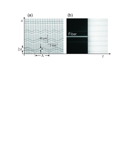
Figure 1: Microscope images (top view) of the sample showing (a) a few set of manufactured coupled optical waveguides, and (b) the fiber coupling geometry for waveguide excitation.

It was previously shown Longhi05 that the evolution of light waves in the optical double-well system is formally equivalent to the dynamics of a periodically-driven nonrelativistic quantum particle in a double-well potential. In the scalar and paraxial approximations, light propagation is described by the equation Vorobeichik03 ; Longhi05

$$i\lambdabar\frac{\partial\psi}{\partial z}=-\frac{\lambdabar^{2}}{2n_{s}}\nabla^{2}_{x,y}\psi+V(x-x_{0}(z),y)\psi.$$ (1)

where: $\lambdabar\equiv\lambda/(2\pi)=1/k$ is the reduced wavelength, $V(x,y)=[n_{s}^{2}-n^{2}(x,y)]/(2n_{s})\simeq n_{s}-n(x,y)$ is the double-well potential, $n(x,y)$ is the refractive index profile of the two-waveguide system, and $n_{s}$ is the reference (substrate) refractive index. The quantum-optical analogy can be retrieved after a Kramers-Henneberger transformation Longhi05 ; Longhi06 $x^{\prime}=x-x_{0}(z)$, $y^{\prime}=y$, $z^{\prime}=z$, $\phi(x^{\prime},y^{\prime},z^{\prime})=\psi(x^{\prime},y^{\prime},z^{\prime})\exp\left[-i(n_{s}/\lambdabar)\dot{x}_{0}(z^{\prime})x^{\prime}-i(n_{s}/2\lambdabar)\int_{0}^{z^{\prime}}d\xi\;\dot{x}_{0}^{2}(\xi)\right]$, where the dot indicates the derivative with respect to $z^{\prime}$, and after elimination of the $y^{\prime}$-dependence of the field $\phi$ using a standard effective index method Chiang86 . Equation (1) is then transformed into the following Schrödinger equation for a particle of mass $n_{s}$ in the double-well potential $V_{e}(x^{\prime})\simeq n_{s}-n_{e}(x^{\prime})$ under the action of a sinusoidal force $F(z^{\prime})$ Longhi05 :

$$i\lambdabar\frac{\partial\phi}{\partial z^{\prime}}=-\frac{\lambdabar^{2}}{2n_{s}}\frac{\partial^{2}\phi}{\partial x^{\prime 2}}+V_{e}(x^{\prime})\phi-Fx^{\prime}\phi\equiv\mathcal{H}_{0}\phi-Fx^{\prime}\phi,$$ (2)

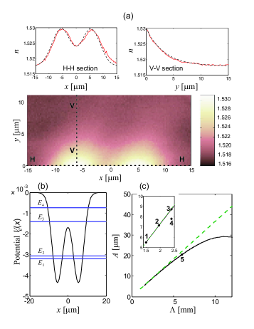
Figure 2: (color online) (a) Measured refractive index profile of the double waveguide system. (b) Computed profile of the effective 1D double-well potential. (c) Manifold of quasi-energy crossing in the $(\Lambda,A)$ plane (solid line). The dashed line has been evaluated from the first zero of the Bessel function using Eq.(3). The inset is an enlargement of the linear portion of the manifold, corresponding to CDT. The five points in the figure correspond to the geometrical parameters of the optical waveguides manufactured in our experiment.

where $n_{e}(x^{\prime})$ is the effective index profile of the waveguide system and $F(z^{\prime})=-n_{s}\ddot{x}_{0}(z^{\prime})=(4\pi^{2}An_{s}/\Lambda^{2})\cos(2\pi z^{\prime}/\Lambda)$ is the ac force. Note that, in the optical analog, the Planck constant is played by the reduced wavelength $\lambdabar$ of photons, whereas the temporal variable of the quantum problem is mapped into the spatial propagation coordinate $z^{\prime}$. CDT is thus simply observed as a suppression of photon tunneling between the two waveguides along the propagation direction.
The refractive index profile $n(x,y)$ has been measured by a refracted-near-field profilometer (Rinck Elektronik) at 670 nm. The measured 2D index profile is depicted in Fig.2(a), together with its section profiles along the horizontal ($HH$) and vertical ($VV$) lines. Figure 2(b) shows the corresponding symmetric double-well potential $V_{e}(x)\simeq n_{s}-n_{e}(x)$ obtained by the effective index approximation. To derive $n_{e}(x)$, the measured 2D index profile $n(x,y)$ was fitted [see dashed curves in Fig.2(a)] by the relation Sharma92 $n(x,y)\simeq n_{s}+\Delta n[g(x-a/2)+g(x+a/2)]f(y)$, where $\Delta n\simeq 0.0124$ is peak index change, $g(x)=[{\rm erf}((x+w)/D_{x})-{\rm}{\rm erf}((x-w)/D_{x})]/[2{\rm erf}(w/D_{x})]$ and $f(y)=\exp(-y/D_{y})$ define the shape of the index profile parallel to the surface of the waveguide ($x$-direction) and perpendicular to the surface ($y$-direction), respectively, $2w\simeq 5\;\mu$m is the channel width and $D_{x}\simeq 4.3\;\mu$m, $D_{y}\simeq 3.3\;\mu$m are the lateral and in-depth diffusion lengths. The numerical computation of the eigenvalues for the Hamiltonian $\mathcal{H}_{0}=-\lambdabar^{2}/(2n_{s})\partial^{2}_{x^{\prime}}+V_{e}(x^{\prime})$ in absence of the driving force indicates that the double-well potential $V_{e}$ supports four bound modes $\xi_{l}(x^{\prime})$ whose energies $E_{l}$ ($l=1,2,3,4$) are depicted in Fig.2(b) by the four horizontal solid lines. The linear combinations $u_{R,L}(x^{\prime})=[\xi_{1}(x^{\prime})\pm\xi_{2}(x^{\prime})]/\sqrt{2}$ of the eigenfunctions $\xi_{1}(x^{\prime})$ and $\xi_{2}(x^{\prime})$ associated to the quasi-degenerate energy levels $E_{1}$ and $E_{2}$ below the barrier correspond to photon localization in the right (R) or in left (L) well of the potential, so that an initial excitation of one of the two wells, obtained by launching the light into either one of the two waveguides, is given approximately by the superposition of the two lowest eigenstates $\xi_{1}(x^{\prime})$ and $\xi_{2}(x^{\prime})$. For the straight waveguides, the field evolution is dominated by the splitting of this doublet, leading to a periodic tunneling of photons between the two waveguides with a spatial period $d_{12}=2\pi\lambdabar/(E_{2}-E_{1})\simeq 7.94$ mm. This is clearly shown in Fig.3(a), where the measured fluorescence pattern corresponding to initial excitation of one of the two waveguides is reported. For the sake of clearness, in the picture the luminosity level of the fluorescence, which decreases with propagation distance due to light absorption, has been gradually rescaled at successive frames. The measured pattern is very well reproduced by a direct numerical simulation of Eq.(1), performed with a standard beam propagation software (BeamPROP 4.0). Higher-order bound modes of the double-well potential shown in Fig.2(b) can be excited by different beam launching conditions. For instance, if the fiber is positioned in the middle between the two waveguides, an excitation of the modes $\xi_{1}(x)$ and $\xi_{3}(x)$ with even symmetry is preferentially attained. In this case, the field evolution is dominated by the splitting of the states $\xi_{1}(x)$ and $\xi_{3}(x)$, leading to a periodic fluorescence pattern with the short spatial period $d_{13}=2\pi\lambdabar/(E_{3}-E_{1})\simeq 545\;\mu$m [see Fig.3(b)].

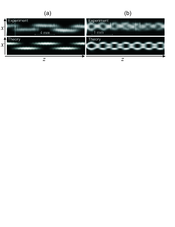
Figure 3: Fluorescence light distribution (top view) in the straight waveguide coupler, and corresponding light intensity distribution predicted by Eq.(1), for different coupling conditions. (a) Excitation of one of the two waveguides; (b) Beam launching in the middle between the two waveguides.

The tunneling dynamics in presence of the external force $F$ strongly depends on the amplitude and (spatial) frequency $\omega=2\pi/\Lambda$ of the force as compared to the energy level spacing of the double-well system Grifoni98 . For instance, at modulation frequencies comparable with the frequency spacing $(E_{3}-E_{2})/\lambdabar$, tunneling is expected to be enhanced. This case was previously demonstrated for a two-waveguide optical system in Ref.Vorobeichik03 . Conversely, CDT occurs approximately for a modulation frequency in the range $(E_{2}-E_{1})\lesssim\lambdabar\omega\lesssim(E_{3}-E_{2})$ and for a modulation amplitude which corresponds to exact crossing between the quasienergies $\epsilon_{1}$ and $\epsilon_{2}$ associated to the lowest tunnel doublet Grifoni98 . In Fig.2(c) the solid curve shows the manifold associated to the exact crossing $\epsilon_{2}=\epsilon_{1}$ in the $(\Lambda,A)$ plane, as numerically computed by means of a two-level approximation of the related driven tunneling problem Grifoni98 ; Grossmann92 . In the high-frequency limit, i.e. for $\lambdabar\omega\gg(E_{2}-E_{1})$ but $\lambdabar\omega<(E_{3}-E_{2})$ to avoid the participation in the dynamics of the third level of energy $E_{3}$, an approximate expression for the quasienergy difference $\Delta\epsilon=\epsilon_{2}-\epsilon_{1}$ reads Grifoni98 ; Grossmann92 ; Longhi05

$$\Delta\epsilon=(E_{2}-E_{1})J_{0}\left(\frac{2\pi\mu_{12}n_{s}A}{\lambdabar\Lambda}\right)$$ (3)

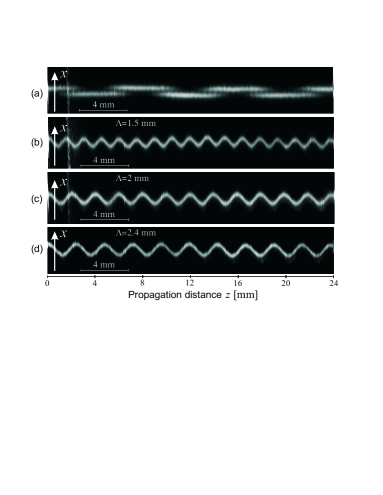
Figure 4: Measured fluorescence light distribution in the ”waveguide” reference frame $(x,z)$ for the straight waveguide coupler (a), and for the three curved waveguide couplers [(b), (c) and (d)] with increasing period $\Lambda$ and amplitude $A$ corresponding to points 1,2 and 3 of Fig.2(c).

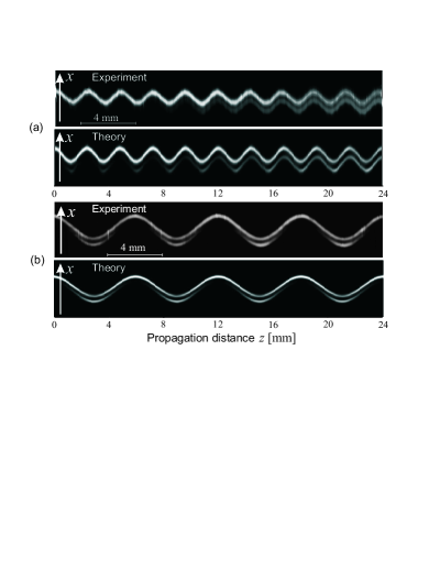
Figure 5: Measured fluorescence light pattern, and corresponding photon density $|\psi(x,0,z)|^{2}$ predicted by Eq.(1), in curved waveguide couplers corresponding to (a) break-up of quasienergy crossing [point 4 in Fig.2(c)], and (b) stroboscopic suppression of tunneling [point 5 in Fig.2(c)].

where $\mu_{12}=\langle\xi_{1}|x|\xi_{2}\rangle$. Considering the first zero of the Bessel function, the condition $\Delta\epsilon=0$ is thus represented by a straight line in the $(\Lambda,A)$ plane, which is depicted by the dashed curve in Fig.2(c). Such a curve, however, deviates from the exact one as $\Lambda$ increases and approaches $4\pi\lambdabar/(E_{2}-E_{1})\simeq 16$ mm, where the solid curve drops toward zero. Crossing of the quasienergies is a necessary -but not a sufficient- condition for the occurrence of CDT. In fact, CDT requires additionally that the degenerate Floquet states at exact energy crossing do not show appreciable amplitude oscillations in one period. A detailed numerical analysis of Eq.(1) shows that CDT indeed occurs along the linear portion of the manifold of Fig.2(c), i.e. for $\Lambda\lesssim 2.5$ mm, which is represented by the enlarged inset in the figure. We experimentally demonstrated the onset of CDT in this portion of the manifold by manufacturing three curved waveguide couplers corresponding to the points 1,2 and 3 of Fig.2(c), i.e. to $\Lambda=1.5$ mm, $A\simeq 5.5\;{\mu}$m (point 1), $\Lambda=2$ mm, $A\simeq 7.3\;{\mu}$m (point 2) and $\Lambda=2.4$ mm, $A\simeq 8.8\;{\mu}$m (point 3). Figure 4 shows the measured fluorescence patterns, as recorded on the CCD camera from the top of the sample, for the straight waveguide coupler and for the three curved waveguide couplers when one of the two waveguides is excited at the input plane. Note that, since the fluorescence is proportional to the local photon density, the patterns in the figure map the profile of $|\psi|^{2}$ in the ”waveguide” reference frame. Therefore, in Figs. 4(b), (c) and (d) the condition for CDT is clearly demonstrated because the photon density follows the sinusoidal bending profile $x_{0}(z)$ of the initially excited well, without tunneling into the adjacent waveguide. We also experimentally checked that the observation of CDT requires that the following two conditions must be simultaneously satisfied: (i) quasienergy crossing, and (ii) absence of appreciable amplitude oscillations of the degenerate Floquet eigenstates within one oscillation period Grifoni98 ; Grossmann92 . As an example, in Fig.5(a) we show the measured fluorescence pattern -and corresponding photon density pattern predicted by the theory- for the curved waveguide coupler corresponding to point 4 of Fig.2(c) ($\Lambda=2.5$ mm and $A=7.9\,\mu$m), in which the condition (i) is not satisfied. Note that in this case the pattern periodicity is broken and tunneling is not suppressed, though the tunneling rate is reduced as compared to the straight waveguide coupler case [compare Fig.4(a) and Fig.5(a)]. Figure 5(b) shows the measured fluorescence pattern for the curved waveguide coupler corresponding to point 5 of Fig.2(c) ($\Lambda=6$ mm and $A\simeq 20.5\;\mu$m). In this case the condition (i) for quasienergy crossing is fulfilled, however over one oscillation period the Floquet eigenstates show non-negligible amplitude oscillations. Though tunneling is suppressed at the stroboscopic distances $z=\Lambda,2\Lambda,...$, over one oscillation period an appreciable fraction of light is observed to tunnel forth and back between the two waveguides. Such a stroboscopic destruction of tunneling can be viewed as a result of destructive interference between successive LZ transitions taking place at periodic level crossings Grifoni98 ; Kayanuma94 , i.e. at the positions $z=\Lambda/4,3\Lambda/4,...$ where $\ddot{x}_{0}=0$. This periodic regime, however, does not correspond to a true CDT Grossmann92 .
In conclusion, we reported on the first visualization of photonic CDT in an optical double-well system which mimics the corresponding quantum-mechanical problem originally proposed in Grossmann91 . The two basic conditions for the observation of CDT, namely quasienergy crossing and absence of amplitude oscillations of the degenerate Floquet doublet, have been experimentally demonstrated.

References

- (1) M. Grifoni and P. Hänggi, Phys. Rep. 304, 229 (1998).
- (2) S. Kohler, J. Lehmann, and P. Hänggi, Phys. Rep. 406, 379 (2005).
- (3) F. Grossmann, T. Dittrich, P. Jung and P. Hänggi, Phys. Rev. Lett. 67, 516 (1991); F. Grossmann, P. Jung, T. Dittrich, and P. Hänggi, Z. Phys. B 84, 315 (1991).
- (4) F. Grossmann, P. Hänggi, Europhys. Lett. 18 (1992) 571.
- (5) W.A. Lin and L.E. Ballentine, Phys. Rev. Lett. 65, 2927 (1990); J. Plata, J.M. Gomez-Llorente, J. Phys. A 25, L303 (1992); M. Holthaus, Phys. Rev. Lett. 69, 1596 (1992).
- (6) R. Utermann, T. Dittrich and P. Hänggi, Phys. Rev. E 49, 273 (1994).
- (7) W.K. Hensinger et al., Nature (London) 412, 52 (2001); D.A. Steck, W.H. Oskay, and M.G. Raizen, Science 293, 274 (2001).
- (8) C. Dembowski, H.-D. Graf, A. Heine, R. Hofferbert, H. Rehfeld, and A. Richter, Phys. Rev. Lett. 84, 867 (2000).
- (9) I. Vorobeichik, E. Narevicius, G. Rosenblum, M. Orenstein, and N. Moiseyev, Phys. Rev. Lett. 90, 176806 (2003).
- (10) Y. Kayanuma, Phys. Rev. A 50, 843 (1994).
- (11) A. Thon, M. Merschdorf, W. Pfeiffer, T. Klamroth, P. Saalfrank, and D. Diesing, Appl. Phys. A 78, 189 (2004).
- (12) Y. Nakamura, Y.A. Pashkin, and J.S. Tsai, Phys. Rev. Lett. 87, 246601 (2001).
- (13) W.D. Oliver et al., Science 310, 1653 (2005).
- (14) M. Sillanpää, T. Lehtinen, A. Paila, Y. Makhlin, and P. Hakonen, Phys. Rev. Lett. 96, 187002 (2006).
- (15) B. J. Keay et al., Phys. Rev. Lett. 75, 4102 (1995).
- (16) K.W. Madison et al., Phys. Rev. Lett. 81, 5093 (1998).
- (17) S. Longhi et al., Phys. Rev. Lett. 96, 243901 (2006).
- (18) S. Raghavan, V.M. Kenkre, D.H. Dunlap, A.R. Bishop, and M.I. Salkola, Phys. Rev. A 54, R1781 (1996).
- (19) S. Longhi, Phys. Rev. A 71, 065801 (2005).
- (20) H. Trompeter et al., Phys. Rev. Lett. 96, 023901 (2006).
- (21) G. Della Valle et al., Electron. Lett. 42, 632 (2006).
- (22) N. Chiodo et al., Opt. Lett. 31, 1651 (2006).
- (23) K.S. Chiang, Appl. Opt. 25, 348 (1986).
- (24) A. Sharma and P. Bindal, Opt. Quant. Electron. 24, 1359 (1992).