Entanglement versus observables

Abstract

A general scheme to seek for the relations between entanglement and observables is proposed in principle. In two-qubit systems with enough general Hamiltonian, we find the entanglement to be the functions of observables for six kinds of chosen state sets and verify how these functions be invariant with time evolution. Moreover, we demonstrate and illustrate the cases with entanglement versus a set of commutable observables under eight kinds of given initial states. Our conclusions show how entanglement become observable even measurable by experiment, and they are helpful for understanding of the nature of entanglement in physics.

Quantum entanglement lies at the heart of quantum mechanics and is viewed as a useful resource in quantum information and quantum computation Gruska . Recently, the relations between quantum entanglement and energy McHugh ; Cavalcanti ; Guhne ; OurCTP as well as physical phenomena Brukner have attracted a lot of attentions from many physicists working in this area. Obviously, these studies and their conclusions are helpful to clearly understand the nature of quantum entanglement and effectively use it in the practical tasks of quantum information processing.

Entanglement indeed relates closely with energy, in particular, for spin Hamiltonian systems. However, their relation is not one to one from our point of view. We prefer to think that this fact indicates quantum entanglement versus quantum obsevables. This is the motivation and propose of our study in this letter.

In fact, for a given state in a Hilbert space $\mathcal{H}$ spanned by all $\{\mbox{$\left|{i}\right\rangle$},i=1,2,\cdots\}$, its entanglement is a function of (perhaps partial) density matrix elements $\rho_{ij}$ as follows

$$E_{q}=f\left(\left\{\rho_{ij}\right\}\right).$$ (1)

When there exists a set of observables $\{\mathcal{O}^{\alpha},\alpha=1,2,\cdots\}$ in the $\mathcal{H}$, and corresponding eigenvectors and eigenvalues of any observable $\mathcal{O}^{\alpha}$ are, respectively, $\left|{v^{\alpha}_{i}}\right\rangle$ and $\lambda^{\alpha}_{i}$ ($i=1,2,\cdots$). Thus, without loss of generality, the given state can be expanded as

$$\rho=\sum_{i,j}\rho_{ij}\mbox{$\left|{i}\right\rangle$}\mbox{$\left\langle{j}\right|$}=\sum_{i,j}a_{ij}^{\alpha}\left(\{\rho_{kl}\})\right)\mbox{$\left|{v^{\alpha}_{i}}\right\rangle$}\mbox{$\left\langle{v^{\alpha}_{j}}\right|$}.$$ (2)

Hence

$$\overline{\mathcal{O}}^{\alpha}={\rm Tr}\left(\mathcal{O}^{\alpha}\rho\right)=\sum_{i}a_{ii}^{\alpha}\left(\{\rho_{kl}\})\right)\lambda^{\alpha}_{i}.$$ (3)

If there are such a set of observables giving an equation system made of the above form equations with various $\alpha$ that we can solve this equation system to obtain all $\rho_{ij}$ appearing at Eq.(1), that is,

$$\rho_{ij}=g_{ij}\left(\left\{\overline{\mathcal{O}}^{\alpha},\left\{\lambda^{\alpha}_{k}\right\}\right\}\right).$$ (4)

Thus, we can build the relation

$$E_{q}=f\left[g_{ij}\left(\left\{\overline{\mathcal{O}}^{\alpha},\left\{\lambda^{\alpha}_{k}\right\}\right\}\right)\right].$$ (5)

This is a general scheme to seek for the relation between entanglement and observables in principle. It is clear that only if this relation is true for a set or a kind of states, it will be really useful and significant because, in the subspace of this set or this kind of states, quantum entanglement becomes observable. Particularly, it will be more interesting and important if this relation is invariant with time evolution and the involved observables are commutable each other.

Now, let we give out six sets of states of two qubits with the above features and the following structures

$$\rho_{1} = \left(\begin{array}[]{llll}a_{1}&0&0&{\rm e}^{-{\rm i}\alpha_{1}}v_{1}\\ 0&0&0&0\\ 0&0&0&0\\ {\rm e}^{{\rm i}\alpha_{1}}v_{1}&0&0&1-a_{1}\end{array}\right),$$ (10)

$$\rho_{2} = \left(\begin{array}[]{llll}0&0&0&0\\ 0&b_{2}&{\rm e}^{-{\rm i}\alpha_{2}}v_{2}&0\\ 0&{\rm e}^{{\rm i}\alpha_{2}}v_{2}&1-{b_{2}}&0\\ 0&0&0&0\end{array}\right),$$ (15)

$$\rho_{3} = \left(\begin{array}[]{llll}0&0&0&0\\ 0&1-{c_{3}}-{d_{3}}&{\rm e}^{-{\rm i}\alpha_{3}}v_{3}&0\\ 0&{\rm e}^{{\rm i}\alpha_{3}}v_{3}&{c_{3}}&0\\ 0&0&0&{d_{3}}\end{array}\right),$$ (20)

$$\rho_{4} = \left(\begin{array}[]{llll}{a_{4}}&0&0&0\\ 0&{b_{4}}&{\rm e}^{-{\rm i}\alpha_{4}}v_{4}&0\\ 0&{\rm e}^{{\rm i}\alpha_{4}}v_{4}&1-{a_{4}}-{b_{4}}&0\\ 0&0&0&0\end{array}\right),$$ (25)

$$\rho_{5} = \left(\begin{array}[]{llll}1-{c_{5}}-{d_{5}}&0&0&{\rm e}^{-{\rm i}\alpha_{5}}v_{5}\\ 0&0&0&0\\ 0&0&{c_{5}}&0\\ {\rm e}^{{\rm i}\alpha_{5}}v_{5}&0&0&{d_{5}}\end{array}\right),$$ (30)

$$\rho_{6} = \left(\begin{array}[]{llll}1-{b_{6}}-{d_{6}}&0&0&{\rm e}^{-{\rm i}\alpha_{6}}v_{6}\\ 0&{b_{6}}&0&0\\ 0&0&0&0\\ {\rm e}^{{\rm i}\alpha_{6}}v_{6}&0&0&{d_{6}}\end{array}\right),$$ (35)

where we have used the Hermi and unit trace properties of the density matrix. As to the positive conditions of them are also required. In order to clearly determine their entanglement by negativity measure n1 ; n2 , we assume all diagonal elements and $v_{i}$ in these density matrices are not negative (negative $v_{i}$ can be rewritten by absorbing its minus sign into ${\rm e}^{\pm{\rm i}\alpha_{i}}$). It is easy to calculate their negativity

$$\begin{array}[]{ll}N_{1}=\left|v_{1}\right|,&\quad N_{2}=\left|v_{2}\right|,\\[6.0pt] N_{3}=\sqrt{d_{3}^{2}+v_{3}^{2}}-d_{3},&\quad N_{4}=\sqrt{a_{4}^{2}+v_{4}^{2}}-a_{4},\\[6.0pt] N_{5}=\sqrt{c_{5}^{2}+v_{3}^{2}}-c_{5},&\quad N_{6}=\sqrt{b_{6}^{2}+v_{4}^{2}}-b_{6}.\end{array}$$ (36)

Introduce the spin tensor for two qubit systems

$$s_{\mu\nu}=\sigma_{\mu}\otimes\sigma_{\nu}\quad(\mu,\nu=0,1,2,3),$$ (37)

where $\sigma_{0}$ is $2\times 2$ identity matrix and $\sigma_{i}$ $(i=1,2,3)$ are the Pauli matrices. Thus, the total spin vector and its square read

$$S_{i} = \frac{1}{2}\left(s_{i0}+s_{0i}\right),\quad S^{2}=\sum_{i=1}^{3}S_{i}S_{i}.$$ (38)

Here, $\hbar$ is taken as 1 for simplicity. Denoting the expected value of an operator $\mathcal{O}$ in the state $\rho_{i}$ by $\langle{\mathcal{O}}\rangle_{i}$, we can express the entanglement by the some components of spin tensor, that is

$$N_{1} = \frac{1}{2}\sqrt{(\langle{s}_{11}\rangle_{1}^{2}+(\langle{s}_{12}\rangle_{1}^{2}},$$ (39)

$$N_{2} = \frac{1}{2}\sqrt{\langle{s}_{11}\rangle_{2}^{2}+\langle{s}_{12}\rangle_{2}^{2}},$$ (40)

$$N_{3} = \frac{1}{2}\sqrt{\langle{s}_{11}\rangle_{3}^{2}+\langle{s}_{12}\rangle_{3}^{2}+\langle{S_{z}}\rangle_{3}^{2}}+\langle{S_{z}}\rangle_{3},$$ (41)

$$N_{4} = \frac{1}{2}\sqrt{\langle{s}_{11}\rangle_{4}^{2}+\langle{s}_{12}\rangle_{4}^{2}+\langle{S_{z}}\rangle_{4}^{2}}-\langle{S_{z}}\rangle_{4},$$ (42)

$$N_{5}\! = \!\frac{1}{2}\sqrt{\langle{s}_{11}\rangle_{5}^{2}\!+\!\langle{s}_{12}\rangle_{5}^{2}\!+\!\left(2\!-\!\langle{S^{2}}\rangle_{5}\right)^{2}}\!+\!\langle{S^{2}}\rangle_{5}\!-\!2,\hskip 28.45274pt$$ (43)

$$N_{6}\! = \!\frac{1}{2}\sqrt{\langle{s}_{11}\rangle_{6}^{2}\!+\!\langle{s}_{12}\rangle_{5}^{2}\!+\!\left(2\!-\!\langle{S^{2}}\rangle_{6}\right)^{2}}\!+\!\langle{S^{2}}\rangle_{6}\!-\!2.$$ (44)

Therefore, the entanglement, for the given six kinds of state sets, can be expressed as the functions of some observables.

It is more interesting how these relations evolute with time. Without loss of generality, the general Hamiltonian of two-qubit systems can be written as

$$H=\sum_{\mu,\nu=0}^{3}h_{\mu\nu}\sigma_{\mu}\otimes\sigma_{\nu}=\sum_{\mu,\nu=0}^{3}h_{\mu\nu}s_{\mu\nu}.$$ (45)

where $h_{\mu\nu}$ are real. Based on the facts that Hamiltonian is made of the spin tensor and that entanglement can expressed as the spin tensor, it is not surprised that there exists the relation between entanglement and energy. However, entanglement quantity and its evolution with time can not be well determined and described by only using energy from our point of view.

It is easy to verify the sufficient conditions to keep the form invariance of time evolution of the above relations (39,40) under the following two kinds form of Hamiltonians

$$H[1] = h_{30}s_{30}+h_{03}s_{03}+f_{1}\left(s_{12}-s_{21}\right)$$ (46)

$$+g_{1}\left(s_{11}+s_{22}\right)+h_{33}s_{33},$$

$$H[2] = h_{30}s_{30}+h_{03}s_{03}+f_{2}\left(s_{12}+s_{21}\right)$$ (47)

$$+g_{2}\left(s_{11}-s_{22}\right)+h_{33}s_{33}.$$

In fact, the verification process is standard and simple. We first expand the density matrix by using the basis made of the eigenvectors of chosen Hamiltonian and their conjugate vectors. Then, acting the time evolution operator (independent of time) on it, we can obtain the final density matrix at a given time. It is key matter to make the final state has the same structure as some $\rho_{i}$. Finally, we calculate its negativity. It is clear that we chose such Hamiltonians (46, 47) and following their simplifications (50)–(55) in order to guarantee the required structure of final state. This is arrived at because these chosen Hamiltonians have appropriate eigenvectors and eigenvalues. The details is omitted in order to save space.

Similarly, we can verify that the relation (41,42) and (43,44) have the form invariance of time evolution, respectively, under $H[1]$ and $H[2]$.

It is more significant if, in the above the relations between entanglement and observables, the involved observables are commutable each other. Actually, this can be obtained by taking particular initial states. Firstly, let us set the initial state as

$$\mbox{$\left|{\psi}\right\rangle$}=\sin\theta_{1}\mbox{$\left|{00}\right\rangle$}+{\rm e}^{-{\rm i}\alpha_{1}}\cos\theta_{1}\mbox{$\left|{11}\right\rangle$}.$$ (48)

Obviously, it is entangled and will evolute to the first kind $\rho_{1}$. Its negativity reads

$$N_{\psi}(t)=\frac{1}{2}\sqrt{1-\langle{S}_{z}\rangle_{2}(t)}.$$ (49)

It is both formally invariant and numerically conversed for the time evolution with $H[1]$, that is, $N_{\psi}(0)=N_{\psi}(t)$. While under $H[2]$, it only keeps invariance in form, but the conversation is broken in general. In order to understand how entanglement evolute, we chose two simplified forms of $H[2]$

$$H[2,1] = \frac{1}{2}\omega_{2}\left(\sigma_{3}\otimes\sigma_{0}-\sigma_{0}\otimes\sigma_{3}\right)$$ (50)

$$+g_{2}\left(\sigma_{1}\otimes\sigma_{1}-\sigma_{2}\otimes\sigma_{2}\right)+h_{2}\sigma_{3}\otimes\sigma_{3},$$

$$H[2,2] = \frac{1}{2}\omega_{2}\left(\sigma_{3}\otimes\sigma_{0}-\sigma_{0}\otimes\sigma_{3}\right)$$ (51)

$$+f_{2}\left(\sigma_{1}\otimes\sigma_{2}+\sigma_{2}\otimes\sigma_{1}\right)+h_{2}\sigma_{3}\otimes\sigma_{3}.$$

Then, let us fix $\alpha_{1}$, for example, $\alpha_{1}=0$, we can draw Fig.1 and Fig.2 to show the surface graphics determined by $\theta$, $\langle S_{z}\rangle(t)$ and $N(t)$.

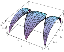
Figure 1: Under $H[2,1]$, $\langle S_{z}\rangle_{\psi}(t)=-\cos\left(2T\right)\cos\left(2\theta_{1}\right)$, $N_{\psi}(t)=\sqrt{1-\cos^{2}\left(2T\right)\cos^{2}\left(2\theta_{1}\right)}/2$ ($\alpha_{1}=0$, $T=2g_{2}$).

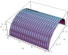
Figure 2: Under $H[2,2]$, $\langle S_{z}\rangle_{\psi}(t)=-\cos\left(2T-2\theta_{1}\right)$, $N_{\psi}(t)=\sqrt{\sin^{2}\left(2T-2\theta_{1}\right)}/2$ ($\alpha_{1}=0$, $T=2f_{2}$).

When the initial state is taken as

$$\mbox{$\left|{\phi}\right\rangle$}=\sin\theta_{2}\mbox{$\left|{01}\right\rangle$}\pm\cos\theta_{2}\mbox{$\left|{10}\right\rangle$},$$ (52)

its negativity reads

$$N_{\phi}(t)=\frac{1}{2}\sqrt{\left(\langle{S^{2}}\rangle(t)-1\right)^{2}}.$$ (53)

It is both formally invariant and numerical conserved only under $H[2]\left(h_{03}=h_{30}\right)$, or only invariant in form under $H[1,2]$. Here, we have defined that

$$H[1,1] = \frac{1}{2}\omega_{1}\left(\sigma_{3}\otimes\sigma_{0}+\sigma_{0}\otimes\sigma_{3}\right)$$ (54)

$$+g_{1}\left(\sigma_{1}\otimes\sigma_{1}+\sigma_{2}\otimes\sigma_{2}\right)+h_{1}\sigma_{3}\otimes\sigma_{3},$$

$$H[1,2] = \frac{1}{2}\omega_{2}\left(\sigma_{3}\otimes\sigma_{0}+\sigma_{0}\otimes\sigma_{3}\right)$$ (55)

$$+f_{1}\left(\sigma_{1}\otimes\sigma_{2}-\sigma_{2}\otimes\sigma_{1}\right)+h_{1}\sigma_{3}\otimes\sigma_{3}.$$

Fig.3 and Fig.4 show the surface graphics determined by $\theta$, $\langle{S}^{2}\rangle(t)$ and $N_{\phi(\pm)}(t)$ under $H[1,2]$.

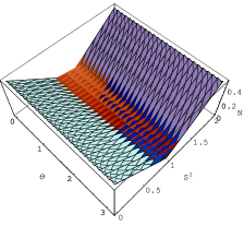
Figure 3: Under $H[1,2]$, $\langle{S}^{2}\rangle_{\phi(+)}(t)=1+\sin^{2}\left(2T+2\theta_{2}\right)$, $N_{\phi(+)}(t)=\sqrt{\sin^{2}\left(2T+2\theta_{2}\right)}/2$ ($\alpha_{2}=0$, $T=2f_{1}$).

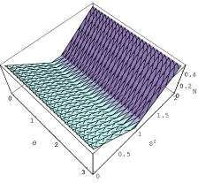
Figure 4: Under $H[1,2]$, $\langle{S}^{2}\rangle_{\phi(-)}(t)=1+\sin^{2}\left(2T-2\theta_{2}\right)$, $N_{\phi(-)}(t)=\sqrt{\sin^{2}\left(2T-2\theta_{2}\right)}/2$ ($\alpha_{2}=\pi$, $T=2f_{1}$).

Similarly, we can obtain the invariance of the relations between the entanglement and observables for the following six kinds of mixed states at the initial time

$$\rho_{1}^{M}(0) = \sin^{2}\theta\mbox{$\left|{00}\right\rangle$}\mbox{$\left\langle{00}\right|$}+\cos^{2}\theta\mbox{$\left|{11}\right\rangle$}\mbox{$\left\langle{11}\right|$},$$ (56)

$$\rho_{2}^{M}(0) = \sin^{2}\theta\mbox{$\left|{01}\right\rangle$}\mbox{$\left\langle{01}\right|$}+\cos^{2}\theta\mbox{$\left|{10}\right\rangle$}\mbox{$\left\langle{10}\right|$},$$ (57)

$$\rho_{3}^{M}(0) = \sin^{2}\theta\mbox{$\left|{10}\right\rangle$}\mbox{$\left\langle{10}\right|$}+\cos^{2}\theta\mbox{$\left|{11}\right\rangle$}\mbox{$\left\langle{11}\right|$},$$ (58)

$$\rho_{4}^{M}(0) = \sin^{2}\theta\mbox{$\left|{01}\right\rangle$}\mbox{$\left\langle{01}\right|$}+\cos^{2}\theta\mbox{$\left|{11}\right\rangle$}\mbox{$\left\langle{11}\right|$},$$ (59)

$$\rho_{5}^{M}(0) = \sin^{2}\theta\mbox{$\left|{00}\right\rangle$}\mbox{$\left\langle{00}\right|$}+\cos^{2}\theta\mbox{$\left|{10}\right\rangle$}\mbox{$\left\langle{10}\right|$},$$ (60)

$$\rho_{6}^{M}(0) = \sin^{2}\theta\mbox{$\left|{01}\right\rangle$}\mbox{$\left\langle{00}\right|$}+\cos^{2}\theta\mbox{$\left|{01}\right\rangle$}\mbox{$\left\langle{01}\right|$}.$$ (61)

They are separable, but they will become entangled after the finite time evolution. Actually, these mixed states can be thought of as the reduced density matrix from the compound systems initially with entanglement. For example, the state $\left(\sin\theta\mbox{$\left|{00}\right\rangle$}+\cos\theta\mbox{$\left|{11}\right\rangle$}\right)\otimes\mbox{$\left|{10}\right\rangle$}$ has entanglement between the first and second qubits. To partially trace qubits 2 and 4, we will get $\rho_{1}^{M}(0)$ made of qubits 1 and 3, or partially trace qubits 1 and 3, we will get $\rho_{3}^{M}(0)$ made of qubits 2 and 4, and so on. This implies that our methods and following discussions can be similarly used to the cases of entanglement transfer and with the environment-system interactions Cavalcanti .

Obviously, $N_{\rho^{M}_{1}}$ under both $H[2,1]$ and $H[2,2]$, $N_{\rho^{M}_{2}}$ under $H[1,2]$ are, respectively,

$$N_{\rho_{1}^{M}}(t) = \frac{1}{2}\sqrt{\langle{S}_{z}\rangle(0)^{2}-\langle{S}_{z}\rangle(t)^{2}},$$ (62)

$$N_{\rho_{2}^{M}}(t) = \frac{1}{2}\sqrt{\left(\langle{S^{2}}\rangle(t)-1\right)^{2}}.$$ (63)

While, under $H[1,2]$

$$N_{\rho_{i}^{M}}(t) = \sqrt{\langle{S}_{z}\rangle_{i}^{2}(t)+\left(\langle{S}^{2}\rangle_{i}(t)+\langle{S}_{z}\rangle_{i}(t)-1\right)^{2}}\hskip 14.22636pt$$ (64)

$$+\langle{S}_{z}\rangle_{i}(t),$$

$$N_{\rho_{j}^{M}}(t) = \sqrt{\langle{S}_{z}\rangle_{j}^{2}(t)+\left(\langle{S}^{2}\rangle_{j}(t)-\langle{S}_{z}\rangle_{j}(t)-1\right)^{2}}$$ (65)

$$-\langle{S}_{z}\rangle_{j}(t),$$

and under both $H[2,1]$ and $H[2,2]$,

$$N_{\rho_{k}^{M}}(t)\!\!\! =\!\!\! \sqrt{\left(2\!-\!\langle{S}^{2}\rangle_{k}(t)\right)^{2}\!+\!\left(\langle{S}^{2}\rangle_{k}(t)\!-\!1\right)^{2}-\langle{S}_{z}\rangle_{k}^{2}(t)}\hskip 14.22636pt$$ (66)

$$+\langle{S}^{2}\rangle_{i}(t)-2,$$

where, $i=3,4$, $j=5,6$ and $k=3,4,5,6$. The surface figures determined by $S_{z}$, $S^{2}$ and $N$ are Figs. 5 - 8

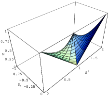
Figure 5: Under $H[1,2]$, $\langle{S}_{z}\rangle_{i}(t)=-\cos^{2}\theta_{i}$, $\langle{S}^{2}\rangle_{i}(t)=\left[3+\cos(2\theta_{i})-(-1)^{i}\sin(2T)\sin^{2}\theta_{i}\right]/2$, $N_{\rho_{i}^{M}}(t)=\sqrt{\cos^{4}\theta_{i}+\sin^{2}(2T)\sin^{4}\theta_{i}}-\cos^{2}\theta_{i}$ ($i=3,4$ and $T=2f_{2}$).

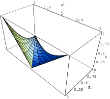
Figure 6: Under $H[1,2]$, $\langle{S}_{z}\rangle_{j}(t)=\sin^{2}\theta_{j}$, $\langle{S}^{2}\rangle_{j}(t)=\left[3-\cos(2\theta_{j})-(-1)^{i}\sin(2T)\cos^{2}\theta_{j}\right]/2$, $N_{\rho_{j}^{M}}(t)=\sqrt{\sin^{4}\theta_{j}+\sin^{2}(2T)\cos^{4}\theta_{j}}-\sin^{2}\theta_{j}$ ($j=5,6$, $T=2f_{2}t$).

Figure 7: Under $H[2,1]$, $\langle{S}_{z}\rangle_{i}(t)\!\!=\!\!-\cos(2T)\sin^{2}\theta_{i}$, $\langle{S}^{2}\rangle_{i}(t)=\left[3+\cos(2\theta_{i})\right]/2$, $N_{\rho_{i}^{M}}(t)=\sqrt{\sin^{4}\theta_{i}+\sin^{2}(2T)\cos^{4}\theta_{i}}-\sin^{2}\theta_{i}$ ($i=3,4$, $T=2f_{1}t$).

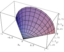
Figure 8: Under $H[2,2]$, $\langle{S}_{z}\rangle_{j}(t)=\cos(2T)\sin^{2}\theta_{j}$, $\langle{S}^{2}\rangle_{j}(t)=\left[3-\cos(2\theta_{j})\right]/2$, $N_{\rho_{j}^{M}}(t)=\sqrt{\cos^{4}\theta_{j}+\sin^{2}(2T)\sin^{4}\theta_{j}}-\cos^{2}\theta_{j}$ ($j=5,6$, $T=2f_{2}t$).

In summary, we propose a general scheme to seek for the relations between entanglement and observables in principle, and we find and verify such relations for the given state sets in two-qubits system, that is, entanglement is expressed as the function of observables. In addition, our methods can be similarly used to the cases of entanglement transfer as well as with the environment-system interaction. Because, Hamiltonian can be expressed by the involved observables, our conclusions have implied the relation between entanglement and energy. Moreover, our conclusions are more determined relations than those derived out by only considering energy. Then we obtain what Hamiltonian will keep their invariance in form with time evolution. This is required to think that entanglement is observable from our point of view. More important and interesting thing in such a claim is that we demonstrate and illustrate that the entanglement can be expressed as the functions of a set of commutable observables $S^{2}$ and $S_{z}$ for eight kinds of initial state sets in two-qubit systems. As well-known, the involved observable should be measurable at the same time. Actually, this means that entanglement can be measured by experiment in these state sets. We expect it will be true in the near future.

We are grateful all the collaborators of our quantum theory group in our university. This work was supported by the National Natural Science Foundation of China under Grant No. 60573008.

References

(1)J. Gruska and H. Imai, Quantum Computing, Osborne McGraw-Hill (1999; updating
2004); M. Nielsen and I. L. Chung, Quantum Computation and
Quantum Information, Cambradge University Press, Canmbridge,
England, (2006)
(2)D. McHugh, M. Ziman, and V. Buz̆ek, Phys. Rev. A74, 042303(2006)
(3)D. Cavalcanti Jr., J. G. Oliveira, J. G. Peixoto de
Faria, M. O. Terra Cunha, and M. F. Santos, Phys. Rev. A74, 042328(2006)
(4)O. Gühne and G. Tóth, Phys. Rev. A74, 052319(2006)
(5)Feng Xu, An Min Wang, Ningbo Zhao, Xiaoqiang Su, and Rengui Zhu,
Commun. Theor. Phys.46 (2006)p591
(6)C. Brukner, V. Vedral and A. Zeilinger, Phys. Rev. A73, 012110(2006)
(7)Karol Zyczkowski, Pawel
Horodecki, Anna Sanpera, and Maciej Lewenstein, Phys. Rev. A 58
(1998) 883
(8)G. Vidal, R.F. Werner, Phys. Rev. A 65, 032314 (2002)