The differential information-geometry of quantum phase transitions

Abstract

The manifold of coupling constants parametrizing a quantum Hamiltonian is equipped with a natural Riemannian metric with an operational distinguishability content. We argue that the singularities of this metric are in correspondence with the quantum phase transitions featured by the corresponding system. This approach provides a universal conceptual framework to study quantum critical phenomena which is differential-geometric and information-theoretic at the same time.

Introduction.– Suppose you are given with a set of quantum states associated to a family of Hamiltonians smoothly depending on a set of parameters, e.g., coupling constants. This parameter manifold – that can include temperature in the case the considered states are thermal ones – is partitioned in regions characterized by the fact that inside them one can “adiabatically” move from one point to the other and no singularities in the expectation values of any observables are encountered. The boundaries between these regular regions are in turn associated to the non-analytic behaviour of some observable and are referred to as critical points; crossing one of these points results in a phase transition (PT). States lying in different regions generally have some strong structural difference and are, in principle, easily distinguishable once somehow a preferred observable is chosen.

The standard machinery, i.e., the so-called Landau-Ginzburg paradigm, to deal with this phenomenon is based on the notions of symmetry breaking, order parameter, and correlation length huang . On the other hand, some system fails to fall in this conceptual framework. This can be due to the difficulty of identifying the proper order parameter for systems whose symmetry breaking pattern is unknown or to the very absence of a local order parameter, e.g., quantum phase transitions (QPTs) involving different kinds of topological order toporder . Even another standard characterization of QPTs, i.e., singularities in the ground state (GS) energy as a function of the coupling constant, misses to capture the boundaries between phases for some QPTs, e.g., those with matrix-product states wo-ci .

In the last few years ideas and tools borrowed from quantum information science qis have been used to study quantum, i.e., zero temperature, phase transistions sachdev ; in particular the role of quantum entanglement in QPTs has been extensively investigated qpt-qis . More recently an approach to QPTs based on the concept of quantum fidelity has been put forward za-pa and applied to systems of quasi-free fermions za-co-gio ; co-gio-za , to the so-called matrix-product states co-ion-za , and extended to finite-temperature zhong-guo . In the fidelity approach, QPTs are identified by studying the behavior of the amplitude of the overlap, i.e., scalar product, between two ground states corresponding to two slightly different set of parameters; at QPTs a drop of the fidelity with scaling behaviour is observed and quantitative information about critical exponents can be extracted co-gio-za ; co-ion-za . The fidelity approach is not based on the identification of an order parameter – and therefore does not require a knowledge of symmetry breaking patterns – or more in general on the analysis of any distinguished observable, e.g., Hamiltonian, but it is a purely metrical one. All the possible observables are in a sense considered at once.

In this paper we shall unveil the universal differential-geometric structure underlying these observations. We shall show how QPTs can be associated to the singularities of a Riemannian metric tensor inherited by the parameter space from the natural Riemannian structure of the projective space of quantum states. This structure has an interpretation in terms of information-geometry woo ; bra-ca providing the differential-geometric approach of this paper with an information-theoretic content.

Information-geometry and QPTs.– Let us consider a smooth family $H(\lambda),\,\lambda\in{\cal M}$(=the parameter manifold), of quantum Hamiltonians in the Hilbert-space $\cal H$ of the system. If $|\Psi_{0}(\lambda)\rangle\in{\cal H}$ denotes the (unique for simplicity) ground-state of $H(\lambda),$ one has defined the map $\Psi_{0}\colon{\cal M}\rightarrow{\cal H}/\lambda\rightarrow|\Psi_{0}(\lambda)\rangle$ associating to each set of parameters the ground-state of the corresponding quantum Hamiltonian. This map can be seen also as a map between ${\cal M}$ and the projective space $P{\cal H}$(=manifold of “rays” of $\cal H$). This space is a metric space being equipped with the so-called Fubini-Study distance $d_{FS}(\psi,\phi):=\cos^{-1}{\cal F}(\psi,\phi)$, where

$${\cal F}(\psi,\phi):=|\langle\psi,\phi\rangle|$$ (1)

and $\|\psi\|=\|\phi\|=1.$ In Ref. woo Wootters showed that this metric has a deep operational meaning: it quantifies the maximum amount of statistical distinguishability between the pure quantum states $|\psi\rangle$ and $|\phi\rangle.$ More precisely, $d_{FS}(\psi,\phi)$ is the maximum over all possible projective measurements of the Fisher-Rao statistical distance between the probability distributions obtained from $|\psi\rangle$ and $|\phi\rangle$ fish . Moreover, this result extends to mixed states as well by replacing the pure-state fidelity (1) with the Uhlmann fidelity Uhlmann and the projective measurements with generalized ones bra-ca .

These results are non-trivial and allow to identifty in a precise manner the Hilbert space geometry with a geometry in the information space: the bigger the Hilbert (or projective) space distance between $|\psi\rangle$ and $|\phi\rangle$ the higher the degree of statistical distinguishability of these two states. From this perspective it is clear that a single real number, i.e., the distance, virtually encodes information about infinitely many observables, e.g., order parameters, one may think to measure. This remark basically contains the main intuition at the basis of the metric approach to QPTs advocated in this paper: at the transition points, a small difference between the control parameters results in a greatly enhanced distinguishability of the corresponding GSs, which should be quantitatively revelead by the behavior of their distance.

For the purposes of this paper it is crucial to note that the projective manifold $P{\cal H}$, besides the structure of metric space, has a well-known structure of Riemannian manifold, i.e., it is equipped with a metric tensor. Here, for the sake of self-consistency, we briefly recall how this Riemannian metric is obtained starting from the Hilbert space structure of $\cal H.$ $P{\cal H}$ can be seen as the base manifold of a (principal) fiber bundle with total space given by the unit ball $S$ of $\cal H$, i.e., $S:=\{|\psi\rangle\in{\cal H}\,/\,||\psi||=1\}$, and projection $\pi\colon S\rightarrow P{\cal H}\,/\,|\psi\rangle\rightarrow\{e^{i\theta}|\psi\rangle\,/\,\theta\in[0,2\pi)\}.$ The tangent space to each point $|\psi\rangle$ of $S$ is isomorphic to a subspace of $\cal H$ and has therefore defined over it the Hermitean bilinear form $g_{|\psi\rangle}(u,v):=\langle u,v\rangle$ ($u$ and $v$ are tangent vectors, i.e., elements of $\cal H$). This defines a (complex) metric tensor field $g$ over $S.$ To project $g$ down to $P{\cal H}$ one has to introduce the notion of horizontal subspace for each tangent space of $S$ or equivalently that of parallel transport and the associated one of connection. In this case the Hilbert space structure of the tangent spaces provides a natural solution to this task: the horizontal subspace is simply the set of vectors $|u\rangle$ which are orthogonal to the fiber over $|\psi\rangle$, i.e., $\langle u,\psi\rangle=0.$ It follows that the complex metric over $P{\cal H}$ is given by $\tilde{g}_{\pi(|\psi\rangle)}(u,v)=\langle u,(1-|\psi\rangle\langle\psi|)v\rangle$, called the quantum geometric tensor pro . The real (imaginary) part of this quantity defines a Riemannian metric tensor (symplectic form) on $P{\cal H}.$ Another, elementary way of getting the form of the Riemannian metric over $P{\cal H}$ is by means of Eq. (1). For $\cal F$ very close to the unity, one can write $d_{FS}^{2}(\psi,\psi+\delta\psi)\simeq 2(1-{\cal F}).$ Since ${\cal F}(\psi,\psi+\delta\psi)\simeq|1+\langle\psi,\delta\psi\rangle+(1/2)\langle\psi,\delta^{2}\psi\rangle|^{2},$ using this expression and the normalization of $|\psi\rangle$ one finds

$$ds^{2}: = d_{FS}^{2}(\psi,\psi+\delta\psi)=\langle\delta\psi,\delta\psi\rangle-|\langle\psi,\delta\psi\rangle|^{2}$$ (2)

$$= \langle\delta\psi,(1-|\psi\rangle\langle\psi|)\delta\psi\rangle\ .$$

What we would like to do now is to see the metric in the parameter manifold $\cal M$ induced, i.e., “pulled-back” by the ground state mapping $\Psi_{0}$ introduced above. By writing $\delta|\Psi_{0}(\lambda)\rangle=\sum_{\mu}|\partial_{\mu}\Psi_{0}\rangle d\lambda^{\mu}$, with $\partial_{\mu}:=\partial/\partial\lambda^{\mu}$, $\mu=1,\ldots,\rm{dim}\,{\cal M}$, and using Eq. (2), one imediately obtains $ds^{2}=\sum_{\mu\nu}g_{\mu\nu}d\lambda^{\mu}d\lambda^{\nu},$ where

$$g_{\mu\nu}=\Re\langle\partial_{\mu}\Psi_{0}|\partial_{\nu}\Psi_{0}\rangle-\langle\partial_{\mu}\Psi_{0}|\Psi_{0}\rangle\langle\Psi_{0}|\partial_{\nu}\Psi_{0}\rangle\ .$$ (3)

Now we provide a simple perturbative argument on why one should expect a singular behavior of the metric tensor at QPTs BPcomment . By using the first order perturbative expansion $|\Psi_{0}(\lambda+\delta\lambda)\rangle\sim|\Psi_{0}(\lambda)\rangle+\sum_{n\neq 0}(E_{0}-E_{n})^{-1}|\Psi_{n}(\lambda)\rangle\langle\Psi_{n}(\lambda)|\delta H|\Psi_{0}(\lambda)\rangle$, where $\delta H:=H(\lambda+\delta\lambda)-H(\lambda)$, one obtains for the entries of the metric tensor (3) the following expression

$$g_{\mu\nu}=\Re\sum_{n\neq 0}\frac{\langle\Psi_{0}(\lambda)|\partial_{\mu}H|\Psi_{n}(\lambda)\rangle\langle\Psi_{n}(\lambda)|\partial_{\nu}H|\Psi_{0}(\lambda)\rangle}{[E_{n}(\lambda)-E_{0}(\lambda)]^{2}}\ .$$ (4)

An analogous expression, with the real part replaced by the imaginary one, gives the antisymmetric tensor which describes the curvature two-form whose holonomy is the Berry phase BP . Continuous QPTs are known to occur when, for some specific values of the parameters and in the thermodynamical limit, the energy gap above the GS closes. This amounts to a vanishing denominator in Eq. (4) that may break down the analyticity of the metric tensor entries.

To get further insight about the physical origin of these singularities we notice that the metric tensor (3) can be cast in an interesting covariance matrix form pro . In the generic case, by moving from $H(\lambda)$ to $H(\lambda+\delta\lambda)$ no level-crossings occur. In this case the unitary operator $O(\lambda,\delta\lambda):=\sum_{n}|\Psi_{n}(\lambda+\delta\lambda\rangle\langle\Psi_{n}(\lambda)|$ “adiabatically” maps the eigenvectors at $\lambda$ onto those at $\lambda+\delta\lambda.$ Then by introducing the observables $X_{\mu}:=i(\partial_{\mu}O)O^{\dagger}$ the metric tensor (3) takes the form $g_{\mu\nu}=(1/2)\langle\{\bar{X}_{\mu},\,\bar{X}_{\nu}\}\rangle$ where $\bar{X}_{\mu}:=X_{\mu}-\langle X_{\mu}\rangle.$ Moreover, the line element $ds^{2}$ can be seen as the variance of the observable $X:=i(dO)O^{\dagger}$, i.e., $ds^{2}=\langle\bar{X}^{2}\rangle.$ The operator $X$ is the generator of the map transforming eigenstates corresponding to different values of the parameter into each other. The smaller the difference between these eigenstates for a given parameter variation, the smaller the variance of $X.$ Intuitively, at the QPT one expects to have the maximal possible difference between $|\Psi_{0}(\lambda)\rangle$ and $|\Psi_{0}(\lambda+\delta\lambda)\rangle$, i.e., many “unperturbed” eigenstates $|\Psi_{n}(\lambda)\rangle$ are needed to build up the “new” GS; accordingly the variance of $X$ can get very large, possibly divergent. In a sense $ds^{2}$ can be seen as a sort of susceptibility of the “order parameter” $X.$

Quasi-Free fermionic systems.– In order to show explicitly how the singularities, i.e., divergencies of $g_{\mu\nu}$ arise, we will discuss the case of the $XY$ model in a detailed fashion; before doing that we would like to make some general considerations about the systems of quasi-free fermions on the basis of the results presented in Ref. za-co-gio . Systems of quasi-free fermions are defined by the following quadratic Hamiltonian

$$H=\sum_{i,j=1}^{L}c_{i}^{\dagger}A_{ij}c_{j}+\frac{1}{2}\sum_{i,j=1}^{L}(c_{i}^{\dagger}B_{ij}c_{j}^{\dagger}+\rm{H.c.})\ ,$$ (5)

where: the $c_{i}$’s ($c_{i}^{\dagger}$’s) are the annihilation (creation) operators of $L$ fermionic modes, $A,B\in M_{L}(\mathbb{R})$ are $L\times L$ real matrices, symmetric and anti-symmetric respectively, i.e., $A^{T}=A,\,B^{T}=-B$. In Ref. za-co-gio it has been shown that the set of GSs of Eq. (5) is parametrized by orthogonal $L\times L$ real matrices $T$ giving the unitary part of the polar decomposition of the matrix $Z:=A-B.$ One can then prove that ${\cal F}(Z,Z^{\prime}):=|\langle\Psi_{Z}|\Psi_{Z^{\prime}}\rangle|=\sqrt{|\det[(T+T^{\prime})/2]|}$ za-co-gio . With no loss of generality we can assume $\det(T)=1$ which identifies the GS manifold of the quasi-free systems (5) with $SO(L,\mathbb{R}).$ Since $f(Z^{\prime}):={\cal F}(Z,Z^{\prime})$ has a maximum equal to one at $Z^{\prime}=Z$ one has $\delta^{2}f(Z^{\prime})|_{Z}=\delta^{2}\ln f(Z^{\prime})|_{Z}$; from this, the expansion for $Z^{\prime}\rightarrow Z$ of the above formula for ${\cal F}$ (Eq. (8) in Ref. za-co-gio ) and by defining $K:=\ln T\in so(L,\mathbb{R}),$ one finds an explicit form for the metric: $ds^{2}\simeq 2(1-{\cal F})=(1/8){\mathrm{Tr}}(dK)^{2}.$ From this equation, if $K=K(\lambda)$, with $\lambda\in{\cal M}$, one obtains the following expression for the metric tensor induced over $\cal M$, i.e., $g_{\mu\nu}=(1/8){\mathrm{Tr}}(\partial_{\mu}K\partial_{\nu}K).$ For translationally invariant Hamiltonians (5) the anti-symmetric matrix $K$ can be always cast in the canonical form $K=i\oplus_{k}\theta_{k}\sigma_{k}^{y}$ where $k$ is a momentum label. Therefore in this important case one has $g_{\mu\nu}=(1/4)\sum_{k}(\partial\theta_{k}/\partial\lambda^{\mu})(\partial\theta_{k}/\partial\lambda^{\nu}).$

We see here that the connection established in Refs. za-co-gio ; co-gio-za ) between QPTs, e.g., due to the vanishing of a quasi-particle energy, and a singularity in the second order expansion of ${\cal F}$ can be directly read as a connection between QPTs in quasi-free systems and singularities in the metric tensor $g_{\mu\nu}.$

The nature of this connection will be now exemplified by considering the QPTs of the periodic antiferromagnetic $XY$ spin chain in a transverse magnetic field. By writing the spin operator in terms of Pauli matrices, i.e., $\bm{S}=\bm{\sigma}/2$, the Hamiltonian for an odd number of spins $L=2M+1$ reads $H=\sum_{j=-M}^{M}[-(1+\gamma)\sigma_{j}^{x}\sigma_{j+1}^{x}/4-(1-\gamma)\sigma_{j}^{y}\sigma_{j+1}^{y}/4+h\sigma_{j}^{z}/2]$, where $\gamma$ is the anisotropy parameter in the $x$-$y$ plane and $h$ is the magnetic field. This Hamiltonian can be cast in the form (5) by the Jordan-Wigner transformation. The critical points of this model are given by the lines ${h}=\pm 1$ and by the segment $|{h}|<1,\gamma=0$. The single particle energies are $\Lambda_{k}=\sqrt{\epsilon_{k}^{2}+\gamma^{2}\sin^{2}(2\pi{}k/L)}$, where $\epsilon_{k}=\cos(2\pi{}k/L)-{h}$ and $k=-M,\dots,M$. For this model the $\theta_{k}$’s defined above have the form $\theta_{k}=\cos^{-1}(\epsilon_{k}/\Lambda_{k})$ and $g_{\mu\nu}=(1/4)\sum_{k=1}^{M}(\partial\theta_{k}/\partial{\lambda^{\mu}})(\partial\theta_{k}/\partial{\lambda^{\nu}})$, where $\lambda^{1,2}=h,\gamma$. One finds $(\partial\theta_{k}/\partial{h})^{2}=\gamma^{2}\sin^{2}{x_{k}}/\Lambda_{k}^{4}$, $(\partial\theta_{k}/\partial\gamma)^{2}=\sin^{2}{x_{k}}(\cos{x_{k}}-{h})^{2}/\Lambda_{\nu}^{4}$, and $(\partial\theta_{k}/\partial{h})(\partial\theta_{k}/\partial\gamma)=\gamma\sin^{2}{x_{k}}(\cos{x_{k}}-{h})/\Lambda_{k}^{4}$, with $x_{k}=2\pi k/L$.

In the thermodynamic limit (TDL), the explicit calculation of $g_{\mu\nu}$ can be performed analytically. Indeed, except at critical points, for large $L$ one can replace the discrete variable $x_{k}$ with a continuous variable $x$ and substitute the sum with an integral, i.e., $\sum_{k=1}^{M}\to[L/(2\pi)]\int_{0}^{\pi}\mathrm{d}x$. At critical points this is not generally feasible due to singularities in some of the terms in the sums. Outside critical points, the resulting integrals, albeit non-trivial, yield simple analytical formulas, which differ depending on whether $|{h}|<1$ or $|{h}|>1$.

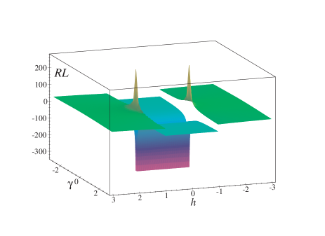
Figure 1: Induced curvature $R$ scaled by the system size $L$ for the parameter space of the $XY$ model.

For $|{h}|<1$ in the TDL one finds a diagonal metric tensor

$$g=\frac{L}{16|\gamma|}\mathrm{diag}\left(\frac{1}{1-{h}^{2}},\frac{1}{(1+|\gamma|)^{2}}\right)$$ (6)

Closed analytic formulas in the TDL can be obtained also for $|{h}|>1$, although in a less compact form, which we omit here for brevity. We only note that for $|{h}|>1$ also the off-diagonal elements of the metric tensor are non-zero. Having the induced metric tensor it is also possible to investigate the induced curvature of the parameter manifold. We therefore compute the scalar curvature $R$, which is the trace of the Ricci curvature tensor Nak . We find $R(|{h}|<1)=-(16/L)(1+|\gamma|)/|\gamma|$ and $R(|{h}|>1)=(16/L)(|{h}|+\sqrt{{h}^{2}+\gamma^{2}-1})/\sqrt{{h}^{2}+\gamma^{2}-1}$. Note that the curvature diverges on the segment $|{h}|\leq 1,\gamma=0$ and is discontinuous on the lines ${h}=\pm 1$. Indeed, $\lim_{|{h}|\to 1^{+}}R=-\lim_{|{h}|\to 1^{-}}R$. The behaviour of the curvature $R$ is shown in Fig. 1.

Mixed states and classical transitions.– In this section we would like to make some extentions of the idea developed in this paper to finite temperature. This will allow us to establish a connection between the present approach and the one for classical PTs developed in ruppy ; brody . This latter formalism is in fact obtained in the special case of commuting density matrices which effectively turns the quantum problem into a classical one.

The fidelity approach to QPTs can be extended to finite-temperature, i.e., to mixed-states, by using the Uhlmann fidelity Uhlmann : ${\cal F}(\rho_{0},\rho_{1}):=\mathrm{Tr}[\rho_{1}^{1/2}\rho_{0}\rho_{1}^{1/2}]^{1/2}.$ When $\rho_{0}$ and $\rho_{1}$ are commuting operators the fidelity takes the form ${\cal F}(\rho_{0},\rho_{1})=\sum_{n}\sqrt{p_{n}^{0}p_{n}^{1}}$ where the $p_{n}^{\alpha}$ are the eigenvalues of the $\rho_{\alpha}$’s rel-ent . In particular, when $\rho_{\alpha}=Z_{\alpha}^{-1}\exp(-\beta_{\alpha}H),Z_{\alpha}:=\mathrm{Tr}\exp(-\beta_{\alpha}H),\,(\alpha=0,1)$ one immediately finds that the fidelity has a simple expression in terms of partition functioms: ${\cal F}=Z(\beta_{0}/2+\beta_{1}/2)(Z(\beta_{0})Z(\beta_{1}))^{-1/2}$ zhong-guo . By expanding for $\beta_{0}=\beta,\beta_{1}=\beta+\delta\beta$ one obtains

$${\cal F}(\beta,\beta+\delta\beta)\simeq\exp\left[-\frac{\delta\beta^{2}}{8\beta^{2}}c_{V}(\beta)\right]$$ (7)

where $c_{V}(\beta)$ denotes the specific heat huang . This relation is remarkable in that it connects the distinguishability degree of two neighboring thermal quantum states directly to the macroscopic thermodynamical quantity $c_{V}.$ The line element of the parameter space, i.e., the $\beta$ axis, is then given by $ds^{2}\sim c_{V}(\beta)\beta^{-2}d\beta^{2}=(\langle H^{2}\rangle_{\beta}-\langle H\rangle^{2}_{\beta})d\beta^{2}.$ A closely related formula has been obtained in ruppy ; brody . Since $PTs$ are associated to anomalies, e.g., divergences, in the behavior of $c_{V}(\beta)$, we see that also in this “classical” case the metric $ds^{2}$ induced on the parameter space contains signatures of the critical points. In this sense the information-geometrical approach to PTs seems able to put quantum and classical PTs under the same conceptual umbrella.

Conclusions.– In this paper we proposed a differential-geometric approach to study quantum phase transtions. The basic idea is that, since distance between quantum states quantitatively encodes their degree of distinguishability, crossing a critical point separating regions with structurally different phases should result in some sort of singular behaviour of the metric. This intuition, based on early studies of quantum fidelity, can be made rigorous in some simple yet important cases, e.g., quasi-free fermion systems. The manifold of coupling constants parameterizing the system’s Hamiltonian can be equipped with a (pseudo) Riemannian tensor $g$ whose singularities correspond to the critical regions. For the case of the $XY$ chain we explicitely computed the components of $g$ in the thermodynamic limit, showing that they are divergent, with universal exponents, at the critical lines. We also computed the scalar curvature of $g$ and analyzed its relation with criticality. The geometrical approach advocated in this paper does not depend on the knowledge of any order parameter or on the analysis of a distinguished observable, it is universal and information-theoretic in nature. The study of the physical meaning of the geometric invariants one can build starting from $g$ (e.g., the curvature), their finite-size as well as scaling behaviour, and their relations with the nature of the quantum phase transition are important questions to be addressed in future research.

References

- (1) K. Huang, Statistical mechanics, John Wiley & Sons, New York, 1987.
- (2) X.G. Wen and Q. Niu, Phys. Rev. B41, 9377 (1990); X.G. Wen, Phys. Rev. Lett. 90, 016803 (2003).
- (3) M.M. Wolf, G. Ortiz, F. Verstraete, and J.I. Cirac, Phys. Rev. Lett. 97, 110403 (2006).
- (4) For a review see, e.g., D.P. DiVincenzo and C.H. Bennett, Nature 404, 247 (2000).
- (5) S. Sachdev, Quantum Phase Transitions (Cambridge University Press, Cambridge, England, 1999).
- (6) T.J. Osborne and M.A. Nielsen, Phys. Rev. A66, 032110 (2002); A. Osterloh, L. Amico, G. Falci, and R. Fazio, Nature 416, 608 (2002); G. Vidal, J.I. Latorre, E. Rico, and A. Kitaev, Phys. Rev. Lett. 90, 227902 (2003); Y. Chen, P. Zanardi, Z.D. Wang, F.C. Zhang, New J. Phys. 8, 97 (2006); L.-A. Wu, M.S. Sarandy, D.A. Lidar, Phys. Rev. Lett. 93, 250404 (2004).
- (7) P. Zanardi and N. Paunkovic, Phys. Rev. E 74, 031123 (2006).
- (8) P. Zanardi, M. Cozzini, and P. Giorda, quant-ph/0606130.
- (9) M. Cozzini, P. Giorda, and P. Zanardi, quant-ph/0608059 (to be published in Phys. Rev. B).
- (10) M. Cozzini, R. Ionicioiu, and P. Zanardi, cond-mat/0611727.
- (11) P. Zanardi, H.-T. Quan, X.-G. Wang, and C.-P. Sun, quant-ph/0612008.
- (12) W.K. Wootters, Phys. Rev. D, 23, 357 (1981).
- (13) S.L. Braunstein and C.M. Caves, Phys. Rev. Lett. 72, 3439 (1994).
- (14) Given the complete set of one-dimensional projections one has the two probability distributions and For and infintesimally close to each other the Fisher distance is given by
- (15) A. Uhlmann, Rep. Math. Phys. 9, 273 (1976); R. Jozsa, J. Mod. Opt. 41, 2315 (1994).
- (16) J.P. Provost and G. Vallee, Commun. Math. Phys. 76, 289 (1980).
- (17) For a reprint collection see Geometric phases in Physics, A. Shapere and F. Wilczek (Eds), World Scientific, Singapore, 1889.
- (18) This heuristic argument is going to be parallel to the one used in Ref. BP-qpt where the relation between QPTs an Berry phases is studied. While the Berry curvature can be identically vanishing, e.g., for real wavefunctions, this cannot be the case for the quantity (3).
- (19) S.-L. Zhu, Phys. Rev. Lett. 96, 077206 (2006); A. Hamma, quant-ph/0602091.
- (20) G. Ruppeiner, Phys. Rev. A 20, 1608 (1979); Rev. Mod. Phys. 67, 605 (1995) and references therein.
- (21) D. Brody and N. Rivier, Phys. Rev. E 51, 1006 (1995).
- (22) See, for example, M. Nakahara, Geometry, topology and Phsyics, Institute of Physics Publishing (1990).
- (23) For () we have that ; thus, to lowest non-zero order, the difference of the fidelity from 1 is proportional to the Fisher-Rao distance, that, for infinitesimal variations, coincides with the relative entropy between the two probability distributions and .