Multiphoton Quantum Optics and
Quantum State Engineering

Abstract

We present a review of theoretical and experimental aspects of multiphoton quantum optics. Multiphoton processes occur and are important for many aspects of matter-radiation interactions that include the efficient ionization of atoms and molecules, and, more generally, atomic transition mechanisms; system-environment couplings and dissipative quantum dynamics; laser physics, optical parametric processes, and interferometry. A single review cannot account for all aspects of such an enormously vast subject. Here we choose to concentrate our attention on parametric processes in nonlinear media, with special emphasis on the engineering of nonclassical states of photons and atoms that are relevant for the conceptual investigations as well as for the practical applications of forefront aspects of modern quantum mechanics. We present a detailed analysis of the methods and techniques for the production of genuinely quantum multiphoton processes in nonlinear media, and the corresponding models of multiphoton effective interactions. We review existing proposals for the classification, engineering, and manipulation of nonclassical states, including Fock states, macroscopic superposition states, and multiphoton generalized coherent states. We introduce and discuss the structure of canonical multiphoton quantum optics and the associated one- and two-mode canonical multiphoton squeezed states. This framework provides a consistent multiphoton generalization of two-photon quantum optics and a consistent Hamiltonian description of multiphoton processes associated to higher-order nonlinearities. Finally, we discuss very recent advances that by combining linear and nonlinear optical devices allow to realize multiphoton entangled states of the electromnagnetic field, either in discrete or in continuous variables, that are relevant for applications to efficient quantum computation, quantum teleportation, and related problems in quantum communication and information.

1 Introduction

In this report we review and discuss recent developments in the physics of multiphoton processes in nonlinear optical media and optical cavities, and their manipulation in the presence of passive and active optical elements. We review as well effective Hamiltonian models and Hamiltonian dynamics of nonquadratic (anharmonic) multiphoton interactions, and the associated engineering of nonclassical states of light beyond the standard coherent and two-photon squeezed states of linear quantum optics.
We present a detailed analysis of the methods and techniques for the production of genuinely quantum multiphoton processes in nonlinear media, and the corresponding models of multiphoton effective nonlinear interactions. Our main goal is to introduce the reader to the fascinating field of quantum nonlinear optical effects (such as, e.g., quantized Kerr interactions, quantized four-wave mixing, multiphoton down conversion, and electromagnetically induced transparency) and their application to the engineering of (generally non Gaussian), nonclassical states of the quantized electromagnetic field, optical Fock states, macroscopic superposition states such as, e. g., optical Schrödinger cat states, multiphoton squeezed states and generalized coherent states, and multiphoton entangled states.
This review is mainly devoted to the theoretical aspects of multiphoton quantum optics in nonlinear media and cavities, and theoretical models of quantum state engineering. However, whenever possible, we tried to keep contact with experimental achievements and the more promising experimental setups proposals. We tried to provide a self-contained introduction to some of the most relevant and appropriate theoretical tools in the physics of multiphoton quantum optics. In particular, we have devoted a somewhat detailed discussion to the recently introduced formalism of canonical multiphoton quantum optics, a systematic and consistent multiphoton generalization of standard one- and two-photon quantum optics. We have included as well an introduction to group-theoretical techniques and nonlinear operatorial generalizations for the definition of some types of nonclassical multiphoton states. Our review is completed by a self-contained discussion of very recent advances that by combining linear and nonlinear optical devices have lead to the realization of some multiphoton entangled states of the electromnagnetic field. This multiphoton entanglement, that has been realized either on discrete or on continuous variables systems, is relevant for applications in efficient quantum computation, quantum teleportation, and related problems in quantum communication and information.
Multiphoton processes occur in a large variety of phenomena in the physics of matter-radiation interactions. Clearly, it is a task beyond our abilities and incompatible with the requirements that a review article should be of a reasonable length extension, and sufficiently self-contained. We thus had to make a selection of topics, that was dictated partly by our personal competences and tastes, and partly because of the rapidly growing importance of research fields including engineering and control of nonclassical states of light, quantum entanglement, and quantum information. Therefore, our review is concerned with that part of multiphoton processes that leans towards the “deep quantum” side of quantum optics, and it does not cover such topics as Rydberg states and atoms, intense fields, multiple ionization, and molecular processes, that are all, in some sense, on the “semiclassical” side of the discipline. Moreover, we have not included sections or discussions specifically devoted to quantum noise, quantum dissipative effects, and decoherence. A very brief “framing” discussion with some essential bibliography on these topics is included in the conclusions.

The plan of the paper is the following. In Section 2 we give a short review of linear quantum optics, introduce the formalism of quasi-probabilities in phase space, and discuss the basics of homodyne and heterodyne detections and of quantum state tomography. In Section 3 we introduce the theory of quantized macroscopic fields in nonlinear media, and we discuss the basic properties of multiphoton parametric processes, including the requirements of energy conservation and phase matching, and the different experimental techniques for the realization of these requirements and for the enhancement of the parametric processes corresponding to higher-order nonlinear susceptibilities. In Section 4 we discuss in detail some of the most important and used parametric processes associated to second- and third-order optical nonlinearities, the realization of concurring interactions, including three- and four-wave mixing, Kerr and Kerr-like interactions, three-photon down conversion, and a first introduction to the engineering of mesoscopic quantum superpositions, and multiphoton entangled states. In Section 5 we describe group theoretical methods for the definition of generalized (multiphoton) coherent states, Hamiltonian models of higher-order nonlinear processes, including degenerate $k$-photon down conversions with classical and quantized pumps, Fock state generation in multiphoton parametric processes, displaced-squeezed number states and Kerr states, intermediate (binomial) states of the radiation field, photon-added and photon-subtracted states, higher-power coherent and squeezed states, and general $n$-photon schemes for the engineering of arbitrary nonclassical states. As already mentioned, in Section 6 we report on a recently established general canonical formulation of multiphoton quantum optics, that allows to introduce multiphoton squeezed states associated to exact canonical structures and diagonalizable Hamiltonians (multiphoton normal modes), we study their two-mode extensions defining non Gaussian entangled states, and we discuss some proposed setups for their experimental realization. In Section 7 we give a bird-eye view on the most relevant theoretical and experimental applications of multiphoton quantum processes and multiphoton nonclassical states in fields of quantum communication and information. Finally, in Section 8 we present our conclusions and discuss future perspectives.

2 A short review of linear quantum optics

In 1927, Dirac [1] was the first to carry out successfully the (nonrelativistic) quantization of the free electromagnetic field, by associating each mode of the radiation field with a quantized harmonic oscillator. Progress then followed with the inclusion of matter-radiation interaction [2], the definition of the general theory of the interacting matter and radiation fields [3, 4], and, after two decades of strenuous efforts, the final construction of divergence-free quantum electrodynamics in its modern form [5, 6, 7, 8, 9, 10, 11]. However, despite these fundamental theoretical achievements and the parallel experimental triumphs in the understanding of electron-photon and atom-photon interactions, only in the sixties, after the discovery of the laser [12], quantum optics entered in its modern era when the theory of quantum optical coherence was systematically developed for the first time by Glauber, Klauder, and Sudarshan [13, 14, 15, 16, 17, 18, 19].
Quantum electrodynamics predicts, and is necessary to describe and understand such fundamental effects as spontaneous emission, the Lamb shift, the laser linewidth, the Casimir effect, and the photon statistics of the laser. The classical theory of radiation fails to account for such effects which can only be explained in terms of the perturbation of the atomic states due to the vacuum fluctuations of the quantized electromagnetic field. Early mathematical developments of quantum electrodynamics have relied heavily on perturbation theory and have assigned a privileged role to the orthonormal basis of Fock number states. Such a formulation is however not very useful nor really appropriate when dealing with coherent processes and structures, like laser beams and nonlinear optical effects, that usually involve large numbers of photons, large-scale space-time correlations, and different types of few- and multi-photon effective interactions. For an exhaustive and comprehensive phenomenological and mathematical introduction to the subjects of quantum optics, see [20, 21, 22, 23, 24, 25, 26, 27, 28, 29, 30].
Before we come to deal with multiphoton processes and multiphoton quantum optics, we need to dedicate the remaining of this Section to a brief review of the physical “one-photon” context in which quantum optics was born. By shortly recalling the theory of optical coherence and a self-contained tutorial on the formalism of coherent states and their properties, this Section will serve as an introduction to the notation and some of the mathematical tools that will be needed in the course of this review.

2.1 Generation of fully coherent radiation: an historical overview

From a classical point of view, the coherence of light is associated with the appearing of interference fringes. The superposition of optical beams with equal frequency and steady phase difference gives rise to an interference pattern, which can be due to temporal or spatial coherence. Traditionally, an optical field is defined to be coherent when showing first-order coherence. The classic interference experiment of Young’s double slit can be described by means of the first-order correlation function, using either classical or quantum theory. The realization of experiments on intensity interferometry and photoelectric counting statistics [31, 32] led to the introduction of higher-order correlation functions. In particular, Hanbury Brown and Twiss [31] verified the bunching effect, showing that the photons of a light beam of narrow spectral width have a tendency to arrive in correlated pairs. A semiclassical approach was used by Purcell [33] to explain the correlations observed in the photoionization processes induced by a light beam. Mandel and Wolf [34] examined the correlations, retaining the assumption that the electric field in a light beam can be described as a classical Gaussian stochastic process. In 1963 came the contributions by Glauber, Klauder and Sudarshan [13, 14, 15, 16, 17, 18, 19] that were essential in opening a new and very fruitful path of theoretical and experimental investigations. Glauber re-introduced the coherent states, first discovered by Schrödinger [35] in the study of the quasi-classical properties of the harmonic oscillator, to study the quantum coherence of optical fields as a cooperative phenomenon in terms of many bosonic degrees of freedom. Here we shortly summarize Glauber’s procedure for the construction of the electromagnetic field’s coherent states [13, 14, 15]. The observable quantities of the electromagnetic field are taken to be the electric and magnetic fields $\vec{E}(\vec{r},t)$ and $\vec{B}(\vec{r},t)$, which satisfy the nonrelativistic Maxwell equations in free space and in absence of sources:

$$\vec{\nabla}\cdot\vec{E}=0\,,\quad\;\vec{\nabla}\cdot\vec{B}=0\,,\quad\;\vec{\nabla}\times\vec{E}=-\frac{\partial\vec{B}}{\partial t}\,,\quad\;\vec{\nabla}\times\vec{B}=\frac{\partial\vec{E}}{\partial t}\;.$$ (1)

Here and throughout the whole report, we will adopt international units with $c=\hbar=1$. The dynamics is governed by the electromagnetic Hamiltonian

$$H_{0}=\frac{1}{2}\int(\vec{E}^{2}+\vec{B}^{2})d^{3}r\;,$$ (2)

and the electric and magnetic fields can be expressed in terms of the vector potential $\vec{A}$:

$$\vec{E}=-\frac{\partial\vec{A}}{\partial t}\,\,\,,\quad\vec{B}=\vec{\nabla}\times\vec{A}\,\,,$$ (3)

where the Coulomb gauge condition $\vec{\nabla}\cdot\vec{A}=0$ has been chosen. Quantization is obtained by replacing the classical vector potential by the operator

$$\vec{A}(\vec{r},t)=\sum_{\vec{k},\lambda}\frac{1}{\sqrt{2\omega_{\vec{k},\lambda}V}}\{a_{\vec{k},\lambda}\hat{\epsilon}_{\vec{k},\lambda}e^{i\vec{k}\cdot\vec{r}-i\omega_{\vec{k},\lambda}t}+a_{\vec{k},\lambda}^{{\dagger}}\hat{\epsilon}_{\vec{k},\lambda}^{*}e^{-i\vec{k}\cdot\vec{r}+i\omega_{\vec{k},\lambda}t}\}\,\,,$$ (4)

with the transversality condition and the bosonic canonical commutation relations given by

$$\vec{k}\cdot\hat{\epsilon}_{\vec{k},\lambda}=0\,\,,\quad\quad[a_{\vec{k},\lambda},a_{\vec{k}^{\prime},\lambda^{\prime}}^{{\dagger}}]=\delta_{\vec{k},\vec{k}^{\prime}}\delta_{\lambda,\lambda^{\prime}}\,,\quad(\hat{\epsilon}_{\vec{k},\lambda}^{*}\cdot\hat{\epsilon}_{\vec{k},\lambda^{\prime}}=\delta_{\lambda,\lambda^{\prime}})\;.$$ (5)

In Eq. (4) $V$ is the spatial volume, $\hat{\epsilon}_{\vec{k},\lambda}$ is the unit polarization vector encoding the wave-vector $\vec{k}$ and the polarization $\lambda$, $\omega_{\vec{k},\lambda}$ is the angular frequency, and $a_{\vec{k},\lambda}$, $a_{\vec{k},\lambda}^{{\dagger}}$ are the corresponding bosonic annihilation and creation operators. Denoting by $\mathbf{k}$ the pair $(\vec{k},\lambda)$, the Hamiltonian (2) reduces to

$$H_{0}\,=\,\sum_{\mathbf{k}}H_{0,\mathbf{k}}\,=\,\frac{1}{2}\sum_{\mathbf{k}}\omega_{\mathbf{k}}(a_{\mathbf{k}}^{{\dagger}}a_{\mathbf{k}}+a_{\mathbf{k}}a_{\mathbf{k}}^{{\dagger}})\;.$$ (6)

Equation (6) establishes the correspondence between the mode operators of the electromagnetic field and the coordinates of an infinite set of harmonic oscillators. The number operator of the $k$-th mode $n_{\mathbf{k}}=a_{\mathbf{k}}^{{\dagger}}a_{\mathbf{k}}$, when averaged over a given quantum state, yields the number of photons present in mode $\mathbf{k}$, i.e. the number of photons possessing a given momentum $\vec{k}$ and a given polarization $\lambda$. The operators $n_{\mathbf{k}}$, $a_{\mathbf{k}}$, and $a_{\mathbf{k}}^{{\dagger}}$, together with the identity operator $I_{\mathbf{k}}$ form a closed algebra, the Lie algebra $h_{4}$, also known as the Heisenberg-Weyl algebra. The single-mode Hamiltonian $H_{0,\mathbf{k}}$ has eigenvalues $E_{\mathbf{k}}=\omega_{\mathbf{k}}\left(n_{\mathbf{k}}+\frac{1}{2}\right)$, $(n_{\mathbf{k}}=0,1,2,...)$. The eigenstates of $H_{0}$ thus form a complete orthonormal basis $\{|n_{\mathbf{k}}\rangle\}$, and are usually known as number or Fock states. The vacuum state $|0_{\mathbf{k}}\rangle$ is defined by the condition

$$a_{\mathbf{k}}|0_{\mathbf{k}}\rangle=0\,,$$ (7)

and the excited states (excited number states) are given by successive applications of the creation operators on the vacuum:

$$|n_{\mathbf{k}}\rangle=\frac{(a_{\mathbf{k}}^{{\dagger}})^{n_{\mathbf{k}}}}{\sqrt{n_{\mathbf{k}}!}}|0_{\mathbf{k}}\rangle\,,\quad(n_{\mathbf{k}}=0,1,2,...)\,.$$ (8)

From Eqs. (3) and (4), the electric field operator can be separated in the positive- and negative-frequency parts

$$\vec{E}(\vec{r},t) = \vec{E}^{(+)}(\vec{r},t)+\vec{E}^{(-)}(\vec{r},t)\,,$$ (9)

$$\vec{E}^{(+)}(\vec{r},t) = i\sum_{\mathbf{k}}\left[\frac{\omega_{\mathbf{k}}}{2V}\right]^{1/2}a_{\mathbf{k}}\hat{\epsilon}_{\mathbf{k}}e^{i(\vec{k}\cdot\vec{r}-\omega_{\mathbf{k}}t)}\,,\quad\vec{E}^{(+){\dagger}}(\vec{r},t)=\vec{E}^{(-)}(\vec{r},t)\;.$$ (10)

The coherent states $|\vec{\varepsilon}\rangle$ of the electromagnetic field are then defined as the right eigenstates of $\vec{E}^{(+)}(\vec{r},t)$, or equivalently as the left eigenstates of $\vec{E}^{(-)}(\vec{r},t)$ :

$$\vec{E}^{(+)}(\vec{r},t)|\vec{\varepsilon}\rangle=\vec{\mathcal{E}}(\vec{r},t)|\vec{\varepsilon}\rangle\,,\quad\langle\vec{\varepsilon}|\vec{E}^{(-)}(\vec{r},t)=\vec{\mathcal{E}}^{*}(\vec{r},t)\langle\vec{\varepsilon}|\,,$$ (11)

where the eigenvalue vector functions $\vec{\mathcal{E}}(\vec{r},t)$ must satisfy the Maxwell equations and may be expanded in a Fourier series with arbitrary complex coefficients $\alpha_{\mathbf{k}}$:

$$\vec{\mathcal{E}}(\vec{r},t)=i\sum_{\mathbf{k}}\left[\frac{\omega_{\mathbf{k}}}{2V}\right]^{1/2}\alpha_{\mathbf{k}}\hat{\epsilon}_{\mathbf{k}}e^{i(\vec{k}\cdot\vec{r}-\omega_{\mathbf{k}}t)}\;.$$ (12)

From Eqs. (11) and (12), it follows that the coherent states are uniquely identified by the complex coefficients $\alpha_{\mathbf{k}}$: $|\vec{\varepsilon}\rangle\equiv|\{\alpha_{\mathbf{k}}\}\rangle$, and, moreover, they are determined by the equations

$$|\{\alpha_{\mathbf{k}}\}\rangle=\prod_{\mathbf{k}}|\alpha_{\mathbf{k}}\rangle,\quad a_{\mathbf{k}}|\alpha_{\mathbf{k}}\rangle=\alpha_{\mathbf{k}}|\alpha_{\mathbf{k}}\rangle,\quad|\alpha_{\mathbf{k}}\rangle=e^{-\frac{|\alpha_{\mathbf{k}}|^{2}}{2}}\sum_{n_{\mathbf{k}}}\frac{\alpha^{n_{\mathbf{k}}}}{\sqrt{n_{\mathbf{k}}!}}|n_{\mathbf{k}}\rangle.$$ (13)

Coherent states possess two fundamental properties, non-orthogonality and over-completeness, expressed by the following relations

$$\langle\alpha_{\mathbf{k}}|\alpha_{\mathbf{k}^{\prime}}\rangle=\exp\left[\alpha_{\mathbf{k}}^{*}\alpha_{\mathbf{k}^{\prime}}-\frac{1}{2}(|\alpha_{\mathbf{k}}|^{2}+|\alpha_{\mathbf{k}^{\prime}}|^{2})\right]\,,$$

$$\int|\{\alpha_{\mathbf{k}}\}\rangle\langle\{\alpha_{\mathbf{k}}\}|\prod_{\mathbf{k}}\pi^{-1}d^{2}\alpha_{\mathbf{k}}=\hat{I}\;,\;\quad d^{2}\alpha_{\mathbf{k}}=dRe[\alpha_{\mathbf{k}}]dIm[\alpha_{\mathbf{k}}]\;,$$ (14)

where $\langle\cdot|\cdot\rangle$ denotes the scalar product, and $\hat{I}$ is the identity operator. Being indexed by a continuous complex parameter, the set of coherent states is naturally over-complete, but one can extract from it any complete orthonormal basis, and, moreover, any arbitrary quantum state $|\psi\rangle$ can still be expressed in terms of continuous superpositions of coherent states:

$$|\psi\rangle=\int f(\{\alpha_{\mathbf{k}}^{*}\})|\{\alpha_{\mathbf{k}}\}\rangle\prod_{\mathbf{k}}\pi^{-1}e^{-|\alpha|^{2}/2}d^{2}\alpha_{\mathbf{k}}\,,$$

$$f(\{\alpha_{\mathbf{k}}^{*}\})=\exp\{\frac{1}{2}\sum_{\mathbf{k}}|\alpha_{\mathbf{k}}|^{2}\}\langle\{\alpha_{\mathbf{k}}\}|\psi\rangle\,.$$ (15)

It is easy to show that the state (13) is realized by the radiation emitted by a classical current. The photon field radiated by an electric current distribution $\vec{J}(\vec{r},t)$ is described by the interaction Hamiltonian

$$H_{I}(t)=-\int\vec{J}(\vec{r},t)\cdot\vec{A}(\vec{r},t)d^{3}r\;,$$ (16)

and thus the associated time-dependent Schrödinger equation is solved by the evolution operator

$$U(t) =\exp\left\{-i\int_{-\infty}^{t}dt^{\prime}\int d^{3}r\vec{J}(\vec{r},t^{\prime})\cdot\vec{A}(\vec{r},t^{\prime})+i\varphi(t^{\prime})\right\}$$ (17)

$$=\prod_{\mathbf{k}}D_{\mathbf{k}}(\alpha_{\mathbf{k}})=\prod_{\mathbf{k}}\exp\{\alpha_{\mathbf{k}}(t)a^{{\dagger}}_{\mathbf{k}}-\alpha^{*}_{\mathbf{k}}(t)a_{\mathbf{k}}\}\;,$$

where $\varphi(t)$ is an overall time-dependent phase factor, the complex time-dependent amplitudes $\alpha_{\mathbf{k}}(t)$ read

$$\alpha_{\mathbf{k}}(t)=\frac{i}{\sqrt{2\omega_{\mathbf{k}}V}}\int_{-\infty}^{t}dt^{\prime}\int d^{3}re^{-i\vec{k}\cdot\vec{r}+i\omega_{\mathbf{k}}t^{\prime}}\hat{\epsilon}_{\mathbf{k}}^{*}\cdot\vec{J}(\vec{r},t^{\prime})\;,$$ (18)

and, finally, the operator $D_{\mathbf{k}}(\alpha_{\mathbf{k}})=\exp\{\alpha_{\mathbf{k}}(t)a^{{\dagger}}_{\mathbf{k}}-\alpha^{*}_{\mathbf{k}}(t)a_{\mathbf{k}}\}$ is the one-photon Glauber displacement operator. Therefore the coherent states of the electromagnetic field are generated by the time evolution from an initial vacuum state under the action of the unitary operator (17). Looking at each of the single-mode contributions in Eq. (17), we see clearly that the interaction corresponds to adding a linear forcing part to the elastic force acting on each of the mode oscillators, and that only one-photon processes are involved. Due to this factorization, the single-mode coherent state $|\alpha_{\mathbf{k}}\rangle$, Eq. (13), associated to the given mode $\mathbf{k}$, is generated by the application of the displacement operator $D_{\mathbf{k}}(\alpha_{\mathbf{k}})$ on the single-mode vacuum $|0_{\mathbf{k}}\rangle$. This can be easily verified by resorting to the Baker-Campbell-Haussdorf relation [23], which in this specific case reads $e^{\alpha_{\mathbf{k}}a^{{\dagger}}_{\mathbf{k}}-\alpha^{*}_{\mathbf{k}}a_{\mathbf{k}}}=e^{-\frac{1}{2}|\alpha_{\mathbf{k}}|^{2}}e^{\alpha_{\mathbf{k}}a_{\mathbf{k}}^{{\dagger}}}e^{-\alpha_{\mathbf{k}}^{*}a_{\mathbf{k}}}$. The decomposition of the electric field in the positive- and negative-frequency parts not only allows to introduce the coherent states in a very natural and direct way, but, moreover, leads, as first observed by Glauber, to the definition of a sequence of $n$-order correlation functions $G^{(n)}$ [14, 15, 36]. Let us consider the process of absorption of $n$ photons, each one polarized in the $\lambda_{j}$ direction $(j=1,...,n)$, and let the electromagnetic field be in a generic quantum state (either pure or mixed) described by some density operator $\rho$. The probability per unit (time)ⁿ that $n$ ideal detectors will record $n$-fold delayed coincidences of photons at points $(\vec{r}_{1},t_{1}),...,(\vec{r}_{n},t_{n})$ is proportional to

$$Tr[\rho E_{\lambda_{1}}^{(-)}(\vec{r}_{1},t_{1})\cdot\cdot\cdot E_{\lambda_{n}}^{(-)}(\vec{r}_{n},t_{n})E_{\lambda_{n}}^{(+)}(\vec{r}_{n},t_{n})\cdot\cdot\cdot E_{\lambda_{1}}^{(+)}(\vec{r}_{1},t_{1})]\,,$$ (19)

where the polarization indices have been written explicitely. Introducing the global variable $x_{j}=(\vec{r}_{j},t_{j},\lambda_{j})$ that includes space, time and polarization, the correlation function of order $n$ is easily defined as a straightforward generalization of relation (19):

$$G^{(n)}(x_{1},...,x_{n},x_{n+1},...,x_{2n})\equiv G^{(n)}(x_{1},...,x_{2n})$$

$$=Tr[\rho E^{(-)}(x_{1})\cdot\cdot\cdot E^{(-)}(x_{n})E^{(+)}(x_{n+1})\cdot\cdot\cdot E^{(+)}(x_{2n})]\;.$$ (20)

These correlation functions are invariant under permutations of the variables $(x_{1}...x_{n})$ and $(x_{n+1}...x_{2n})$ and their normalized forms are conveniently defined as follows:

$$g^{(n)}(x_{1},...,x_{2n})=\frac{G^{(n)}(x_{1},...,x_{2n})}{\prod_{j=1}^{2n}\left\{G^{(1)}(x_{j},x_{j})\right\}^{1/2}}\;,$$ (21)

so that, by definition, the necessary condition for a field to have a degree of coherence equal to $n$ is

$$|g^{(m)}(x_{1},...,x_{2m})|=1\,,$$ (22)

for every $m\leq n$. As $g^{(n)}(x_{1},...,x_{n};x_{n},...,x_{1})$ is a positive-defined function, other two alternative, but equivalent, conditions for having coherence of order $n$ are:

$$g^{(m)}(x_{1},...,x_{m};x_{m},...,x_{1})=1\;,$$

$$G^{(m)}(x_{1},...,x_{m};x_{m},...,x_{1})=\prod_{i=1}^{m}G^{(1)}(x_{i},x_{i})\;,$$ (23)

for every $m\leq n$. Relations (22), or (23), are only necessary conditions for $n$-order coherence, and mean that the detection rate of $m$-fold delayed coincidences is equal to the products of the detections rates of each photon counter. For a completely coherent field, i.e., coherent at any arbitrary order, the following equivalent conditions must be satisfied:

$$|g^{(n)}(x_{1},...,x_{2n})|=1\;,$$

$$|G^{(n)}(x_{1},...,x_{2n})|=\prod_{j=1}^{2n}\left\{G^{(1)}(x_{j},x_{j})\right\}^{1/2}\;,\quad n=1,2,...\;.$$ (24)

Relations (24) indicate that an even stronger definition of coherence can be adopted, by assuming the full factorization of $G^{(n)}$ in terms of a complex function $\mathcal{E}(x)$ of the global space-time-polarization variable:

$$G^{(n)}(x_{1},...,x_{n},x_{n+1},...,x_{2n})=\mathcal{E}^{*}(x_{1})\cdot\cdot\cdot\mathcal{E}^{*}(x_{n})\mathcal{E}(x_{n+1})\cdot\cdot\cdot\mathcal{E}(x_{2n})\,.$$ (25)

Coherent states defined by Eq. (11) imply the complete factorization of the correlation functions, see e.g. [13, 14, 15], and hence they describe a fully coherent radiation field. Let us consider in more detail the normalized second-order correlation function $g^{(2)}$. This correlation is of particular importance when dealing with the problem of discriminating the classical and the genuinely quantum, or “nonclassical” in the quantum optics jargon, statistical properties of a state. Let us consider only two modes $a_{j}$ $(j=1,2)$ of the field with frequencies $\omega_{j}$; then, the normalized second order correlation function corresponding to the probability of counting a photon in mode $i$ at time $t$ and a photon in mode $j$ at time $t+\tau$ can be expressed in terms of the creation and annihilation operators in the form:

$$g_{ij}^{(2)}(t,t+\tau)=\frac{\langle a_{i}^{{\dagger}}(t)a_{j}^{{\dagger}}(t+\tau)a_{i}(t)a_{j}(t+\tau)\rangle}{\langle a_{i}^{{\dagger}}(t)a_{i}(t)\rangle\langle a_{j}^{{\dagger}}(t+\tau)a_{j}(t+\tau)\rangle}\;,\quad(i,j=1,2)\;,$$ (26)

where the notation is self-explanatory. For stationary processes (processes invariant under time translations) $g^{(2)}$ is independent of $t$, i.e. $g^{(2)}(t,t+\tau)=g^{(2)}(0,\tau)\equiv g^{(2)}(\tau)$. For zero time delay, we thus have

$$g_{ij}^{(2)}(0)=\frac{\langle a_{i}^{{\dagger}}a_{j}^{{\dagger}}a_{i}a_{j}\rangle}{\langle a_{i}^{{\dagger}}a_{i}\rangle\langle a_{j}^{{\dagger}}a_{j}\rangle}\,.$$ (27)

In the case of a single-mode field, the equivalent relations are obtained by eliminating the subscripts $i$ and $j$. For a coherent state, all the correlation functions $g^{(n)}(\tau)=1$ at any order $n$, and, in particular, $g^{(2)}(\tau)=1$. However, for a generic state $g^{(2)}(\tau)\neq 1$ and the behavior of the normalized second order correlation function is related to the so-called bunching or antibunching effects [37]. In fact, for classical states photons exhibit a propensity to arrive in pairs at a photodetector (bunching effect); deviations from this tendency are then a possible signature of a genuinely nonclassical behavior (antibunching effect: photons are revealed each at a time at the photodetector). If one looks at second order correlation functions, bunching is favored if $g^{(2)}(\tau)<g^{(2)}(0)$, while antibunching is favored when $g^{(2)}(\tau)>g^{(2)}(0)$ [37]. Since $\lim_{\tau\rightarrow\infty}g^{(2)}(\tau)=1$, i.e. the probability of joint detection coincides with the probability of independent detection, a field for which $g^{(2)}(0)<1$ will always exhibit photon antibunching on some time scale. As an example, let us consider a single-mode, pure number state described by the (projector) density operator $\rho_{n}=|n\rangle\langle n|$, and a one-mode thermal state described by the density operator $\rho_{th}=\sum_{n}\frac{\bar{n}^{n}}{(1+\bar{n})^{n+1}}|n\rangle\langle n|$, where $\bar{n}$ denotes the average number of thermal photons. These two states both enjoy first-order coherence: $|g_{n}^{(1)}(0)|=|g_{th}^{(1)}(0)|=1$, but it is easy to verify that $g_{th}^{(2)}(0)=2$ while $g_{n}^{(2)}(0)=\left\{\begin{array}[]{cc}1-\frac{1}{n}&(n\geq 2)\,,\\ 0&(n=0,1)\,.\end{array}\right.$
Then, the normalized second order correlation function discriminates between the classical character of the thermal state and the genuinely quantum nature of the number states that exhibit antibunching. Similar results are obtained for two-mode states by looking at the two-mode cross-correlation functions. For a two-mode thermal state, described by the density operator $\rho_{2th}=\sum_{n_{1},n_{2}}\frac{\bar{n_{1}}^{n_{1}}}{(1+\bar{n_{1}})^{n_{1}+1}}\frac{\bar{n_{2}}^{n_{2}}}{(1+\bar{n_{2}})^{n_{2}+1}}|n_{1},n_{2}\rangle\langle n_{1},n_{2}|$, the second-order degree of coherence for the $i$-th mode is given by $g_{ii}^{(2)}(0)=2$, while the intermode cross-correlation is $g_{12}^{(2)}(0)=1$; therefore, for two-mode thermal states, the direct- and cross-correlations satisfy the classical Cauchy-Schwartz inequality [38]

$$g_{11}^{(2)}(0)g_{22}^{(2)}(0)>[g_{12}^{(2)}(0)]^{2}\;.$$ (28)

On the contrary , for a two-mode number state $|n_{1},n_{2}\rangle\langle n_{1},n_{2}|$ $(n_{i}\geq 2)$, we have $g_{ii}^{(2)}(0)=1-\frac{1}{n_{i}}$ $(i=1,2)$ and $g_{12}^{(2)}(0)=1$. Consequently, the nonclassicality of the state emerges via the violation of the Cauchy-Schwartz inequality for the direct- and the cross-correlations:

$$g_{11}^{(2)}(0)g_{22}^{(2)}(0)=1-\frac{n_{1}+n_{2}-1}{n_{1}n_{2}}<1=[g_{12}^{(2)}(0)]^{2}\;.$$ (29)

The most suitable framework for the description of the dynamical and statistical properties of the quantum states of the radiation field is established by introducing characteristic functions and appropriate quasi-probability distributions in phase space [13, 16, 42], that, among many other important properties, allow to handle and compute expectation values of any kind of observable built from ordered products of field operators. We will introduce and make use of some of the most important quasi-probability distributions later on, but here we anticipate some remarks on the phase-distribution function that Glauber and Sudarshan [13, 16] first introduced as the $P$-function representation of the density operator by the equivalence

$$\rho=\int P(\{\alpha_{\mathbf{k}}\})|\{\alpha_{\mathbf{k}}\}\rangle\langle\{\alpha_{\mathbf{k}}\}|\prod_{\mathbf{k}}d^{2}\alpha_{\mathbf{k}}\;.$$ (30)

In particular, Sudarshan proved that, for any state $\rho$ of the quantized electromagnetic field, any expectation value of any normally ordered operatorial function of the field operators $\mathcal{O}_{N}(\{a^{{\dagger}}_{\mathbf{k}}\},\{a_{\mathbf{k}}\})$ can be computed by means of a complex, classical distribution functional:

$$Tr[\mathcal{O}_{N}(\{a^{{\dagger}}_{\mathbf{k}}\},\{a_{\mathbf{k}}\})\rho]=\prod_{\mathbf{k}}\int d^{2}\alpha_{\mathbf{k}}\mathcal{O}_{N}(\{\alpha^{*}_{\mathbf{k}}\},\{\alpha_{\mathbf{k}}\})P(\{\alpha_{\mathbf{k}}\})\;.$$ (31)

The correspondence between the quantum-mechanical and classical descriptions, defined by the complex functional $P(\{\alpha_{\mathbf{k}}\})$, is at the heart of the optical equivalence theorem [16, 18], stating that the complete quantum mechanical description contained in the density matrix can be recovered in terms of classical quasi-probability distributions in phase space, as we will see in more detail in the following.

2.2 More about coherence at any order, one-photon processes and coherent states

The theory of coherent states marks the birth of modern quantum optics; it provides a convenient mathematical formalism, and at the same time it constitutes the standard of reference with respect to the degree of nonclassicality of any generic quantum state of the electromagnetic field. For this reason, we review here some fundamental properties of the coherent states, restricting the treatment to a single mode $a_{\mathbf{k}}$ of the radiation field, and dropping the subscript $\mathbf{k}$. The coherent states can be constructed using three different, but equivalent, definitions, each of them shedding light on some of their most important physical properties.

a)

The coherent states $|\alpha\rangle$ are eigenstates of the annihilation operator $a$. The quadrature representation $\psi_{\alpha}(x_{\lambda})$ of the coherent state $|\alpha\rangle$, defined as the overlap between the quadrature eigenstate $|x_{\lambda}\rangle$ and $|\alpha\rangle$: $\psi_{\alpha}(x_{\lambda})=\langle x_{\lambda}|\alpha\rangle$, can be easily determined by solving the eigenvalue equation $\langle x_{\lambda}|a|\alpha\rangle=\alpha\psi_{\alpha}(x_{\lambda})$. Expressing the annihilation operator in terms of the quadrature operators

$$X_{\lambda}=\frac{e^{-i\lambda}a+e^{i\lambda}a^{{\dagger}}}{\sqrt{2}}\;,\quad P_{\lambda}=X_{\lambda+\frac{\pi}{2}}\;,\;\quad[X_{\lambda},P_{\lambda}]\,=\,i\;,$$ (32)

the eigenvalue equation $\langle x_{\lambda}|a|\alpha\rangle=\alpha\psi_{\alpha}(x_{\lambda})$ can be expressed in the quadrature representation in the form

$$\frac{e^{i\lambda}}{\sqrt{2}}\left(x_{\lambda}+\frac{\partial}{\partial x_{\lambda}}\right)\psi_{\alpha}(x_{\lambda})=\alpha\psi_{\alpha}(x_{\lambda})\;.$$ (33)

Its normalized solution is

$$\psi_{\alpha}(x_{\lambda}) \,=\, \pi^{-1/4}e^{-\frac{1}{2}|\alpha|^{2}}e^{-\frac{1}{2}x_{\lambda}^{2}+\sqrt{2}e^{-i\lambda}\alpha x_{\lambda}-\frac{1}{2}e^{-2i\lambda}\alpha^{2}}$$ (34)

$$= \pi^{-1/4}e^{-\frac{i}{2}\langle X_{\lambda}\rangle\langle X_{\lambda+\pi/2}\rangle}e^{i\langle X_{\lambda+\pi/2}\rangle x_{\lambda}}e^{-\frac{1}{2}(x_{\lambda}-\langle X_{\lambda}\rangle)^{2}}\;,$$

with $\langle X_{\lambda}\rangle=\langle\alpha|X_{\lambda}|\alpha\rangle=\frac{\alpha e^{-i\lambda}+\alpha^{*}e^{i\lambda}}{\sqrt{2}}$. Therefore coherent states are Gaussian in $x_{\lambda}$, in the sense that they are characterized by a Gaussian probability distribution $|\psi_{\alpha}(x_{\lambda})|^{2}$, and thus are completely specified by the knowledge of the first and second statistical moments of the quadrature operators. The free evolution of the wave packet (34) is given by $|\alpha(t)\rangle=e^{-it\omega a^{{\dagger}}a}|\alpha\rangle=|e^{-i\omega t}\alpha\rangle$, and the corresponding expectation values of the quadrature operators are $\langle X\rangle(t)=\sqrt{2}Re[\alpha e^{i\omega t}]$, $\langle P\rangle(t)=\sqrt{2}Im[\alpha e^{i\omega t}]$. Hence, the coherent states $|\alpha(t)\rangle$ preserve the shape of the initial wave packet at any later time, and the expectation values of the quadrature operators evolve according to the classical dynamics of the pure harmonic oscillator.

b)

The coherent states can be obtained by applying the Glauber displacement operator $D(\alpha)$ on the vacuum state of the quantum harmonic oscillator, $|\alpha\rangle=D(\alpha)|0\rangle$.

c)

The coherent states are quantum states of minimum Heisenberg uncertainty,

$$\langle\Delta X_{\lambda}^{2}\rangle\langle\Delta P_{\lambda}^{2}\rangle=\frac{1}{4}\;,$$ (35)

where

$$\langle\Delta F^{2}\rangle\equiv\langle F^{2}\rangle-\langle F\rangle^{2}\;,$$ (36)

and, moreover,

$$\langle\Delta X_{\lambda}^{2}\rangle=\langle\Delta P_{\lambda}^{2}\rangle=\frac{1}{2}\;.$$ (37)

The three definitions $a)$, $b)$, $c)$ are equivalent, in the sense that they define the same class of coherent states. Later on, we will see that the equivalence between the three definitions breaks down when generalized coherent states will be defined for algebras more general than the Heisenberg-Weyl algebra of the harmonic oscillator.

Let us consider now the photon number probability distribution $P(n)$ for the coherent state $|\alpha\rangle$, i.e. the probability that $n$ photons are detected in the coherent state $|\alpha\rangle$. It is easy to see that it is a Poisson distribution:

$$P(n)\equiv|\langle n|\alpha\rangle|^{2}=e^{-|\alpha|^{2}}\frac{|\alpha|^{2n}}{n!}\;.$$ (38)

The average number of photons $\langle n\rangle$ in the state $|\alpha\rangle$ is therefore $\langle n\rangle=|\alpha|^{2}$, with variance $\langle\Delta n^{2}\rangle=\langle n\rangle$. Since the second order correlation function, for zero time delay, can be easily expressed in terms of the number operator as

$$g^{(2)}(0)=1+\frac{\langle\Delta n^{2}\rangle-\langle n\rangle}{\langle n\rangle^{2}}\;,$$ (39)

we obtain for a coherent state, as expected, $g^{(2)}(0)=1$. From the previous discussions it follows that coherent states are, as anticipated, ”classical” reference states, in the sense that they share some statistical aspects together with truly classical states of the radiation field, such as a positive defined quasi-probability distribution, a Poissonian photodistribution, and photon bunching. Thus, they can be used as a standard reference for the characterization of the nonclassical nature of other states, as, for instance, measured by deviations from Poissonian statistics. In particular, a state with a photon number distribution narrower than the Poissonian distribution (which implies $g^{(2)}(0)<1$) is referred to as sub-Poissonian, while if $g^{(2)}(0)>1$ (corresponding to a photon number distribution broader than Poissonian distribution), it is referred as super-Poissonian. It is clear that the phenomena of sub-Poissonian statistics and photon antibunching are closely related, because the first one implies the second for some time scale. However, the reverse statement cannot be established in general. In order to clarify this point, let us consider a generic stationary field distribution, for which it can be shown that [39]

$$\langle\Delta n^{2}\rangle-\langle n\rangle=\frac{\langle n\rangle^{2}}{T^{2}}\int_{-T}^{T}d\tau(T-|\tau|)[g^{(2)}(\tau)-1]\;,$$ (40)

where $T$ is the counting interval. It is then possible for a state realizing such a distribution, to be such that $g^{(2)}(\tau)>g^{(2)}(0)$, but still with super-Poissonian statistics. A detailed review on these subtleties and on sub-Poissonian processes in quantum optics has been carried out by Davidovich [40]. Another important signature of nonclassicality has been introduced by Mandel, who defined the $Q$ parameter [41]

$$Q=\frac{\langle\Delta n^{2}\rangle-\langle n\rangle}{\langle n\rangle}\,,$$ (41)

as a measure of the deviation of the photon number statistics from the Poissonian distribution. The interpretation of $Q$ is straightforward with respect to the field statistics.

2.3 Quasi-probability distributions, homodyne and heterodyne detection, and quantum state tomography

The classical or nonclassical character of a state can be tested on more general grounds by resorting to quasi-probability distributions in phase space. As already mentioned, the prototype of these distributions is the $P$-function defined by Eq. (30), which provides the diagonal coherent state representation [13, 16]

$$P(\alpha,\alpha^{*})=Tr[\rho\delta(\alpha^{*}-a^{{\dagger}})\delta(\alpha-a)]\;.$$ (42)

Here the Dirac $\delta$-function of an operator is defined in the usual limiting sense in vector spaces. For a coherent state $|\beta\rangle$ the $P$-representation is then the two-dimensional delta function over complex numbers, $\delta^{(2)}(\alpha-\beta)$, and this relation suggests a possible definition of nonclassical state: “If the singularities of $P(\alpha)$ are of types stronger than those of delta functions, i.e. derivatives of delta function, the state represented will have no classical analog” [15]. Besides the $P$-function, other distribution functions associated to different orderings of $a$ and $a^{{\dagger}}$ can be defined. A general quasi-probability distribution in phase space $W(\alpha,p)$ is defined as the two-dimensional Fourier transform of the corresponding $p-$ordered characteristic function $\chi(\xi,p)$ [42, 23]:

$$W(\alpha,p)=\frac{1}{\pi^{2}}\int_{-\infty}^{\infty}d^{2}\xi\chi(\xi,p)e^{\alpha\xi^{*}-\alpha^{*}\xi},\quad\chi(\xi,p)=Tr[\rho e^{\xi a^{{\dagger}}-\xi^{*}a}]e^{p|\xi|^{2}/2},$$ (43)

where $\alpha$ and $\xi$ are complex variables, and $p=1,0,-1$ correspond, respectively, to normal, symmetric and antinormal ordering [42, 23] in the product of bosonic operators. Moreover, it can been shown that $W(\alpha,p)$ is normalized and real for all complex $\alpha$ and real $p$. Statistical moments of any $p-$ordered product of annihilation and creation operators $a$ and $a^{{\dagger}}$ can be obtained exploiting the relation

$$\langle a^{{\dagger}m}a^{n}\rangle_{p}=\int_{-\infty}^{\infty}d^{2}\alpha W(\alpha,p)\alpha^{*m}\alpha^{n}\;.$$ (44)

For $p=1$, $W(\alpha,1)$ reduces to the Glauber-Sudarshan $P$ distribution; for $p=-1$, $W(\alpha,-1)$ defines the Husimi distribution $Q(\alpha)=\frac{1}{\pi}\langle\alpha|\rho|\alpha\rangle$ [43]. Finally, for $p=0$, $W(\alpha,0)=W(\alpha)$ defines the Wigner distribution [44, 45]. The Wigner distribution can be viewed as a joint distribution in phase space for the two quadrature operators $X_{\lambda}$ and $P_{\lambda}$ and can be written in the form

$$W(x_{\lambda},p_{\lambda})=\frac{1}{\pi}\int dye^{-2ip_{\lambda}y}\langle x_{\lambda}+y|\rho|x_{\lambda}-y\rangle\;.$$ (45)

The probability distribution for the quadrature component $X_{\lambda}$ is given by $\frac{1}{2}\int dp_{\lambda}W(x_{\lambda},p_{\lambda})$, and an equivalent, corresponding definition holds as well for the quadrature $P_{\lambda}$. In order to obtain a classical-like description and equip them with the meaning of true joint probability distributions in classical phase space, the Wigner functions $W(\alpha)$ should be nonnegative defined. In fact, in general the Wigner function can take negative values, in agreement with the basic quantum mechanical postulate on the complementarity of canonically conjugated observables. However, it is easy to see that $W(\alpha)$ is non negative for all Gaussian states, and thus, in particular, for coherent states. Therefore, another important measure of nonclassicality can be taken to be the negativity of $W(x_{\lambda},p_{\lambda})$ [46]. This criterion turns out to be of practical importance, after Vogel and Risken succeeded to show that the Wigner function can be reconstructed from a set of measurable quadrature-amplitude distributions, achieved by homodyne detection [47].
In quantum optics, homodyne detection is a fundamental technique for the measurement of quadrature operators $X_{\lambda}$ of the electromagnetic field [48, 49]. The scheme of a balanced homodyne detection is depicted in Fig. (1).

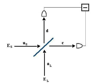
Figure 1: Scheme of a homodyne detector.

Two electromagnetic field inputs of the same frequency $\omega$, a signal field $E^{(+)}_{S}\propto a_{S}\;e^{-i\omega t}\;$ and a strong coherent laser beam $E^{(+)}_{L}\propto a_{L}\;e^{-i\omega t}\;$ (local oscillator), enter the two input ports of a beam splitter. The input modes $a_{S}$ and $a_{L}$ are converted in the output modes $c$ and $d$ by the unitary transformation $U_{BS}$:

$$\left(\begin{array}[]{c}c\\ d\\ \end{array}\right)\,=\,U_{BS}\left(\begin{array}[]{c}a_{S}\\ a_{L}\\ \end{array}\right)\;,\quad U_{BS}=\left(\begin{array}[]{cc}\sqrt{\eta}&\sqrt{1-\eta}e^{i\delta}\\ -\sqrt{1-\eta}e^{-i\delta}&\sqrt{\eta}\\ \end{array}\right)\;,$$ (46)

where $\eta$ is the transmittance of the beam splitter, and $\delta$ is the phase shift between transmitted and reflected waves. The detected difference of the output intensities $\langle I\rangle=\langle c^{{\dagger}}c\rangle-\langle d^{{\dagger}}d\rangle$ is

$$\langle I\rangle=(1-2\eta)(\langle a^{{\dagger}}_{L}a_{L}\rangle-\langle a^{{\dagger}}_{S}a_{S}\rangle)+2\sqrt{\eta(1-\eta)}\langle e^{-i\delta}a_{S}^{{\dagger}}a_{L}+e^{i\delta}a_{S}a_{L}^{{\dagger}}\rangle\;.$$ (47)

If the local oscillator mode $a_{L}$ can be approximated by an intense coherent field of complex amplitude $\alpha_{L}$ ($a_{L}\rightarrow\alpha_{L}$), exploiting $|\alpha_{L}|^{2}\gg\langle a^{{\dagger}}_{S}a_{S}\rangle$, the difference current can be written in the form

$$\langle I\rangle\,\approx\,(1-2\eta)|\alpha_{L}|^{2}+\sqrt{2\eta(1-\eta)}|\alpha_{L}|\langle X_{\xi-\delta}\rangle\;,$$ (48)

where $\xi=\arg\alpha_{L}$, and $X_{\xi-\delta}$ is the quadrature operator $X_{\lambda}$, associated to the signal mode $a_{S}$, with $\lambda\equiv\xi-\delta$. Exploiting the freedom in tuning the angles $\xi$ and $\delta$, the mean amplitude of any quadrature phase operator can be measured. Thus, the homodyne detector allows the direct experimental measurement of the field quadratures. Now, as shown in Ref. [47], the Wigner function, corresponding to a state $\rho$ of the signal mode $a_{S}$, can be reconstructed via an inverse Radon transform from the quadrature probability distribution $p(x,\lambda)\doteq\langle x_{\lambda}|\rho|x_{\lambda}\rangle$, which in turn is determined by the homodyne measurements. This procedure for the recontruction of a quantum state is the core of the so-called quantum homodyne tomography. It has been widely studied, refined, and generalized [50, 51, 52], and experimentally implemented in several different instances [53, 54, 55, 56]. One can show that the Wigner function can be written as the inverse Radon transform of $p(x,\lambda)$ in the form

$$W(x,y)\,=\,\int_{0}^{\pi}\frac{d\lambda}{\pi}\int_{-\infty}^{\infty}dx^{\prime}p(x^{\prime},\lambda)\int_{-\infty}^{\infty}\frac{dk}{4}e^{ik(x^{\prime}-x\cos\lambda-y\sin\lambda)}\;.$$ (49)

A further aim of quantum tomography is to estimate, for arbitrary quantum states, the average value $\langle\mathcal{O}\rangle$ of a generic operator $\mathcal{O}$. This expectation can be computed as

$$\langle\mathcal{O}\rangle\,=\,\int_{0}^{\pi}\frac{d\lambda}{\pi}\int_{-\infty}^{\infty}dxR[\mathcal{O}](x,\lambda)\;,$$ (50)

where the estimator $R[\mathcal{O}](x,\lambda)$ is given by

$$R[\mathcal{O}](x,\lambda)\,=\,Tr[\mathcal{O}K(X_{\lambda}-x)]\;,$$ (51)

and

$$K(x)\,\equiv\,\int_{-\infty}^{\infty}(dk/4)\exp(ikx)\,=\,-\mathcal{P}[1/(2x^{2})]\;,$$

where $\mathcal{P}$ denotes the Cauchy principal value.

For the sake of completeness, we briefly outline the description of another detection method, the so-called heterodyne detection [57, 58]. It allows simultaneous measurements of two orthogonal quadrature components, whose statistics is described by the Husimi $Q$-function. Heterodyne detection can be realized by the following device. The signal field and another field, the auxiliary field, feed the same port of a beam splitter, as depicted in Fig.(2). Moreover, as in the case of homodyne detection, a local field oscillator enters the other port of the beam splitter.

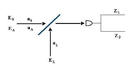
Figure 2: Scheme of heterodyne detector.

In this configuration, at variance with the homodyne instance, the frequencies of the signal, auxiliary and local oscillator fields are different. The signal field $E_{S}$ is associated to the mode $a_{S}$ at the frequency $\omega_{S}$, the auxiliary field $E_{A}$ is associated to the mode $a_{A}$ at the frequency $\omega_{A}$, and the local oscillator field $E_{L}$ is associated to the mode $a_{L}$ at the frequency $\Omega_{L}$, where

$$\omega_{S}\,+\,\omega_{A}\,=\,2\Omega_{L}\;,\quad\omega_{S}\,-\,\omega_{A}\,=\,2\Omega\;,\quad\Omega_{L}\,\gg\,\Omega\;.$$ (52)

A broadband detector is placed in one output port of the beam splitter to detect beats at the frequency $\Omega\ll\Omega_{L}$. After demodulation, the time dependent components, proportional to $\cos(\Omega t)$ and $\sin(\Omega t)$, can be detected simultaneously, yielding the measured variable

$$Z\,\equiv\,Z_{1}+iZ_{2}\,=\,a_{S}\otimes I_{a_{A}}\,+\,I_{a_{S}}\otimes a_{A}^{{\dagger}}\;.$$ (53)

It is to be remarked that, formally, the same quantum measurement can be obtained by a double homodyne detection.

3 Parametric processes in nonlinear media

The advent of laser technology allowed to begin the study of nonlinear optical phenomena related to the interaction of matter with intense coherent light, and extended the field of conventional linear optics (classical and quantum) to nonlinear optics (classical and quantum). Historically, the fundamental events, which marked such a passage, were the realization of the first laser device (a pulsed ruby laser) in 1960 [12] and the production of the second harmonic, through a pulsed laser incident on a piezoelectric crystal, in 1961 [59].
As the main body of this report will be concerned with quantum optical phenomena in nonlinear media, relevant for the generation of nonclassical multiphoton states, this Section is dedicated to a a self-contained, yet somewhat detailed discussion of the basic aspects of nonlinear optics that are of importance in the quantum domain. For a much more thorough and far more complete examination of the classical aspects of nonlinear optics the reader is referred to Refs. [60, 61, 62, 63, 64].
All linear and nonlinear optical effects arise in the processes of interaction of electromagnetic fields with matter fields. The physical characteristics of the material system determine its reaction to the radiation; therefore, the effect on the field can provide information about the system. On the other hand, the medium can be used to generate a new radiation field with particular features. Harmonic generation, wave mixing, self-focusing, optical phase-conjugation, optical bistability, and in particular optical parametric amplification and oscillation, can all be described by studying the properties of a fundamental object, the nonlinear polarization. For this reason, we will dedicate this Section to review the essential notions of nonlinear quantum optics, including the general description of optical field-induced electric polarization, the standard phenomenological quantization procedures, the effective Hamiltonians associated to two- and three-wave mixing processes, and the theory of the nonlinear susceptibilities. We will pay much attention to the lowest order processes, i.e. second and third order processes, which will be widely used in the next Section, and we will finally discuss the properties and the relative orders of magnitude of the different nonlinear susceptibilities.

Let us begin by considering a system constituted by an atomic medium and the applied optical field; the Hamiltonian of the whole system can be written as

$$H=H_{0}+H_{I}(t)\;,$$ (54)

where $H_{0}$ is the unperturbed Hamiltonian of the medium without an applied field and $H_{I}(t)$ is the matter-radiation interaction part. Considering, for simplicity, only the interaction between an outer-shell electron and the applied optical field, the interaction operator takes the form [60]

$$H_{I}(t)=-\frac{e}{2m_{e}}(\vec{p}_{e}\cdot\vec{A}+\vec{A}\cdot\vec{p}_{e})+\frac{e^{2}}{2m_{e}}\vec{A}\cdot\vec{A}+eV\;,$$ (55)

where $e$ and $m_{e}$ are the charge and the mass of the electron, $\vec{p}_{e}$ is the momentum operator of the electron, and $\vec{A}$ and $V$ are the vector and the scalar potential of the optical field. Choosing the Coulomb gauge so that $\vec{\nabla}\cdot\vec{A}=0$ and $V=0$, and neglecting the smaller diamagnetic quadratic term $\vec{A}\cdot\vec{A}$, we get

$$H_{I}(t)=-\frac{e}{m_{e}}\vec{A}\cdot\vec{p}_{e}\;.$$ (56)

For optical fields the wavelength is generally much larger than the molecular radius; as a consequence, the electric-quadrupole and the magnetic-dipole contributions can be neglected and the interaction Hamiltonian (56) reduces to the electric-dipole interaction:

$$H_{I}(t)=-\vec{p}\cdot\vec{E}(t)\;,$$ (57)

where $\vec{p}=e\,\vec{r}$ is the microscopic electric dipole vector of a single atom. The meaning, the applicability and the different properties of the interactions (56) and (57) have been discussed at length in the literature [65, 66, 67, 68, 69, 70, 71, 72], and it turns out that the vast majority of nonlinear optical processes can be adequately described by applying the electric-dipole approximation to the matter-radiation interaction Hamiltonian. The interaction is considered within a polarizable unit of the material system, that is a volume in which the electromagnetic field can be assumed to be uniform at any given time. In a solid this volume is large in comparison with the atomic dimensions, but small with respect to the wavelength of the optical field. As the field is uniform within a polarizable unit, the radiation interaction looks like that of an electric dipole in a constant field, and the electric-dipole approximation is fully justified in the spectral region going from the far-infrared to the ultraviolet; for shorter wavelengths $\vec{E}$ cannot be assumed to be uniform over atomic dimensions. When applicable, the electric-dipole approximation allows to identify the nonlocal macroscopic polarization with the local, macroscopic electric-dipole polarization $\vec{P}(t)\equiv\sum_{i=1}^{N}\vec{p}_{i}(t)$, given by the sum of all the $N$ induced atomic dipole moments that constitute the dielectric medium. The macroscopic polarization is in general a complicated nonlinear function of the electric fields; however, in the electric-dipole approximation, it is possible to describe the polarization and the dynamics of radiation in material media with the help of the dielectric susceptibilities, to be defined in the following. In particular, it is possible to expand the macroscopic dielectric polarization in a power series of the electric field amplitudes [60, 61, 62, 63, 64]:

$$\vec{P}(t)=\vec{P}^{(1)}(t)+\vec{P}^{(2)}(t)+...+\vec{P}^{(n)}(t)+...\;,$$ (58)

where the the generic term $\vec{P}^{(n)}(t)$ in the power series expansion reads, for each spatial component $P_{j}^{(n)}(t)$ ($j=1,2,3$),

$$P_{j}^{(n)}(t)=\int_{0}^{\infty}...\int_{0}^{\infty}d\tau_{1}...d\tau_{n}R_{j\alpha_{1}...\alpha_{n}}^{(n)}(\tau_{1},...,\tau_{n})E_{\alpha_{1}}(t-\tau_{1})...E_{\alpha_{n}}(t-\tau_{n}).$$ (59)

Here the subscript $\alpha_{i}$ is a short-hand notation for the spatial and polarization components of the electric field vector $\vec{E}$ at time $t-\tau_{i}$, the object $R_{j\alpha_{1}\alpha_{2}...\alpha_{n}}^{(n)}(\tau_{1},\tau_{2},...,\tau_{n})$ is the $j$-th spatial component of the $n$-th order response function, a tensor of rank $(n+1)$, that takes into account the reaction of the medium to the applied electromagnetic field. In Eqs. (58) and (59) only the temporal dependence is retained, while the spatial dependence is not explicitated for ease of notation. Moreover, it is assumed that the medium reacts only by a local response, that is the polarization at a point is completely determined by the electric field at that same point. Moving from the time domain to the frequency domain, Eq. (59) becomes

$$P_{j}^{(n)}(\omega)=\chi_{j\alpha_{1}\alpha_{2}...\alpha_{n}}^{(n)}(\omega_{\sigma};\omega_{1},...,\omega_{n})E_{\alpha_{1}}(\omega_{1})...E_{\alpha_{n}}(\omega_{n})\,,$$ (60)

where $\omega_{\sigma}=\sum_{i=1}^{n}\omega_{i}$, and the $n$-th order nonlinear susceptibility tensor is defined by

$$\chi_{j\alpha_{1}...\alpha_{n}}^{(n)}(\omega_{\sigma};\omega_{1},...,\omega_{n})$$

$$=\int...\int d\tau_{1}...d\tau_{n}\Theta(\tau_{1})...\Theta(\tau_{n})R^{(n)}_{j\alpha_{1}...\alpha_{n}}(\tau_{1},...,\tau_{n})e^{i(\omega_{1}\tau_{1}+...+\omega_{n}\tau_{n})}\;,$$ (61)

where $\Theta$ is the Heaviside step function. For a lossless, nondispersive and uniform medium, the susceptibilities $\underline{\chi}^{(n)}$ are symmetric tensors of rank $(n+1)$, while the polarization vector $\vec{P}$ provides the macroscopic description of the interaction of the electromagnetic field with matter [61]. There are various physical mechanisms which are responsible for nonlinear polarization responses in the medium [60]: the distortion of the electronic clouds, the intramolecular motion, the molecular reorientation, the induced acoustic motion, and the induced population changes. For our purposes, here and in the following only the first two mechanisms will have to be taken into account.

3.1 Quantized macroscopic fields in nonlinear dielectric media

Several approaches have been proposed for the quantization of the electromagnetic field in nonlinear, inhomogeneous, or dispersive media [73, 74, 75, 76, 77, 78, 79, 80, 81, 82, 83, 84, 85, 86, 87, 88]. The standard phenomenological macroscopic quantum theory, widely used in nonlinear optics, was formulated by Shen [75] and was later elaborated by Tucker and Walls [76] for the description of parametric frequency conversion. Classical electrodynamics in a dielectric medium is described by the macroscopic Maxwell equations

$$\vec{\nabla}\cdot\vec{D}=\rho_{ext}\,,$$ (62)

$$\vec{\nabla}\times\vec{E}=-\frac{\partial\vec{B}}{\partial t}\,,$$ (63)

$$\vec{\nabla}\cdot\vec{B}=0\,,$$ (64)

$$\vec{\nabla}\times\vec{B}=\frac{\partial\vec{D}}{\partial t}+\vec{J}_{ext},$$ (65)

where $\vec{D}=\vec{E}+\vec{P}$ is the displacement field, $\rho_{ext}$ and $\vec{J}_{ext}$ represent charge and current sources external to the dielectric medium, $\vec{P}$ is the polarization of the medium, and Heaviside-Lorentz units have been used throughout. We can also write the polarization, whose $j$-th component is given by Eq. (60), in the more synthetic form

$$\vec{P}=\underline{\chi}^{(1)}:\vec{E}+\underline{\chi}^{(2)}:\vec{E}\vec{E}+\underline{\chi}^{(3)}:\vec{E}\vec{E}\vec{E}+...\;,$$ (66)

where the first term denotes the contraction of the electric field vector with the first-order susceptibility tensor $\underline{\chi}^{(1)}$ (which is a tensor of rank $2$), the second term denotes the contraction of two electric field vectors with the second-order susceptibility tensor $\underline{\chi}^{(2)}$ (a tensor of rank $3$), the third term denotes the contraction of three electric field vectors with the third-order susceptibility tensor $\underline{\chi}^{(3)}$ (a tensor of rank $4$), and so on. Equations (64), (63), (62), (65) and (66) constitute the basis of the theory of nonlinear optical effects in matter. The standard method to derive a macroscopic quantum theory is to quantize the macroscopic classical theory. The Hamiltonian is

$$H=H_{0}+H_{I}=\frac{1}{2}\int d^{3}r[\vec{E}^{2}+\vec{B}^{2}]-\int d^{3}r\vec{E}\cdot\vec{P}\;.$$ (67)

The first term is the free quadratic Hamiltonian $H_{0}$, while the second term $H_{I}$ represents the interaction in the medium. Recalling the expression of the polarization vector $\vec{P}$ in terms of the electric fields and of the susceptibilities, one sees that the interaction Hamiltonian contains, in principle, nonlinear, anharmonic terms of arbitrary order. The lowest-order, cubic power of the electric field in the interaction Hamiltonian, is associated to the second-order susceptibility $\underline{\chi}^{(2)}$. The standard phenomenological quantization is achieved by introducing the vector potential operator (4), where $\omega_{\vec{k},\lambda}=c|\vec{k}|/n_{\vec{k},\lambda}$ is the angular frequency in the medium ($n_{\vec{k},\lambda}$ being the index of refraction). Effective Hamiltonians associated to nonlinear quasi-steady-state processes of different orders are widely used in quantum optics, and are based on this simple quantization procedure. However there are some difficulties with this theory; the most serious one being inconsistency with Maxwell equations. For instance, it is easy to verify that Eqs. (3) and the Coulomb condition $\vec{\nabla}\cdot\vec{A}=0$ imply that, in absence of external charges, $\vec{\nabla}\cdot\vec{E}=0$ rather than $\vec{\nabla}\cdot\vec{D}=0$, and, moreover, Eq. (63) is not satisfied. In the following we review the main progresses achieved to overcome such inconsistencies and to provide an exhaustive and consistent formulation of quantum electrodynamics in nonlinear media. A first successful solution to the shortcomings of the standard quantization scheme has been introduced by Hillery and Mlodinow [78], who assume the displacement field $\vec{D}$ as the canonical variable for quantization in a homogeneous and nondispersive medium. Starting from an appropriate Lagrangian density, they introduce the interaction Hamiltonian

$$H_{I}=\int d^{3}r\left(\frac{1}{2}\chi_{ij}^{(1)}E_{i}E_{j}+\frac{2}{3}\chi_{ijk}^{(2)}E_{i}E_{j}E_{k}+\frac{3}{4}\chi_{ijkl}^{(3)}E_{i}E_{j}E_{k}E_{l}+...\right),$$ (68)

where $\vec{E}$ and $\vec{B}$ are to be considered as functions of $\vec{A}$ and $\vec{D}$. Performing a mode expansion, annihilation (and creation) operators can be defined by

$$a_{\vec{k},\lambda}(t)=\int d^{3}re^{-i\vec{k}\cdot\vec{r}}\hat{\epsilon}_{\vec{k},\lambda}\left(\sqrt{\frac{\omega_{\vec{k}}}{2V}}\vec{A}(\vec{r},t)-\frac{i}{\sqrt{2\omega_{\vec{k}}V}}\vec{D}(\vec{r},t)\right)\;.$$ (69)

It is easy to check that these newly defined annihilation and creation operators obey the bosonic canonical commutation relations (5). It is also important to notice that, as $a_{\vec{k},\lambda}(t)$ depends on $\vec{D}$, it contains both field and matter degree of freedom. One can introduce a further, alternative quantization procedure [78] by redefining the four-vector potential, the so-called ”dual potential” $\Lambda=(\Lambda_{0},\vec{\Lambda})$:

$$\vec{D}=\vec{\nabla}\times\vec{\Lambda}\,,\quad\vec{B}=\frac{\partial\vec{\Lambda}}{\partial t}+\vec{\nabla}\Lambda_{0}\;.$$ (70)

Expressing the polarization in a more convenient form:

$$\vec{P}=\underline{\eta}^{(1)}:\vec{D}+\underline{\eta}^{(2)}:\vec{D}\vec{D}+\underline{\eta}^{(3)}:\vec{D}\vec{D}\vec{D}+...\;,$$ (71)

where the quantities $\eta$ can be expressed uniquely in terms of the susceptibilities $\chi$, one can derive the following canonical Hamiltonian density

$$H= \frac{1}{2}(\vec{B}^{2}+\vec{D}^{2})-\frac{1}{2}\vec{D}\cdot\underline{\eta}^{(1)}:\vec{D}-\frac{1}{3}\vec{D}\cdot\underline{\eta}^{(2)}:\vec{D}\vec{D}$$ (72)

$$-\frac{1}{4}\vec{D}\cdot\underline{\eta}^{(3)}:\vec{D}\vec{D}\vec{D}-...-\vec{B}\cdot\vec{\nabla}\Lambda_{0}\;.$$

The gauge condition can be chosen so that $\Lambda_{0}=0$ and $\vec{\nabla}\cdot\vec{\Lambda}=0$. The theory can be quantized in the same way as the free quantum electrodynamics, and the commutation relations are

$$[\dot{\Lambda}_{i}(\vec{r},t),\Lambda_{j}(\vec{r}^{\prime},t)]=i\delta_{ij}^{tr}(\vec{r}-\vec{r}^{\prime})\;,$$ (73)

where $\delta_{ij}^{tr}(\vec{r})=\frac{1}{(2\pi)^{3}}\int d^{3}k\left(\delta_{ij}-\frac{k_{i}k_{j}}{|\vec{k}|^{2}}\right)e^{i\vec{k}\cdot\vec{r}}$ is the transverse delta function. In this theory, however, some problems arise with operator ordering, and it is difficult to include dispersion. However, as shown by Drummond [81], this quantization method can be generalized to include dispersion, by resorting to a field expansion in a slowly varying envelope approximation, including an arbitrary number of envelopes, and assuming lossless propagation in the relevant frequency bands. The final quantum Hamiltonian is written in terms of creation and annihilation operators corresponding to group-velocity photon-polariton excitations in the dielectric.
Concerning nonlinear and inhomogeneous media, we briefly discuss a general procedure for quantization [88] that extends the approach of Glauber and Lewenstein [82]. This method is based on the assumption of medium-independent commutation relations for the fields $\vec{D}$ and $\vec{B}$, which from Eqs. (64) and (63) (for the source-free case) can be expanded in terms of a complete set of transverse spatial functions $\{\vec{f}_{\vec{k},\lambda}(\vec{r})\}$ and $\{\vec{\nabla}\times\vec{f}_{\vec{k},\lambda}(\vec{r})\}$:

$$\vec{D}(\vec{r},t)=-\sum_{\vec{k},\lambda}\Pi_{\vec{k},\lambda}(t)\vec{f}^{*}_{\vec{k},\lambda}(\vec{r})\;,\quad\vec{B}(\vec{r},t)=\sum_{\vec{k},\lambda}Q_{\vec{k},\lambda}(t)\vec{\nabla}\times\vec{f}_{\vec{k},\lambda}(\vec{r})\;.$$ (74)

Both the functions $\vec{f}_{\vec{k},\lambda}$ and the operatorial coefficients $Q$ and $\Pi$ satisfy Hermiticity conditions: $\vec{f}_{\vec{k},\lambda}^{*}=\vec{f}_{-\vec{k},\lambda}$, $Q_{\vec{k},\lambda}^{{\dagger}}=Q_{-\vec{k},\lambda}$, and $\Pi_{\vec{k},\lambda}^{{\dagger}}=\Pi_{-\vec{k},\lambda}$. Moreover, the spatial functions satisfy transversality, orthonormality, and completeness conditions, and the commutation relations read

$$[Q_{\vec{k},\lambda}(t),\Pi_{\vec{k}^{\prime},\lambda^{\prime}}(t)]=i\delta_{\vec{k}\vec{k}^{\prime}}\delta_{\lambda\lambda^{\prime}}\;.$$ (75)

The energy density and the Hamiltonian of the electromagnetic field in the medium are given by

$$dU(\vec{r},t)=\vec{E}(\vec{r},t)\cdot d\vec{D}(\vec{r},t)+\vec{H}(\vec{r},t)\cdot d\vec{B}(\vec{r},t),\quad H=\int d^{3}rU(\vec{r},t).$$ (76)

Finally, being $H$ a functional of $\vec{D}$ and $\vec{B}$, the full field quantization is obtained from Eqs. (74) and (75).

3.2 Effective Hamiltonians and multiphoton processes

In this Subsection, by applying the standard quantization procedure to Hillery and Mlodinow’s Hamiltonian (68) treated in the rotating wave approximation, we will show how to obtain various phenomenological Hamiltonian models describing effective multiphoton processes in nonlinear media. The electric contribution to the electromagnetic energy in the nonlinear medium, Eq. (68), can be written in the form

$$H=\int_{V}d^{3}r\left[\frac{1}{2}E^{2}(\vec{r},t)+\sum_{n}X_{n}(\vec{r},t)\right],$$

$$X_{n}(\vec{r},t)=\frac{n}{n+1}\underline{\chi}^{(n)}:\vec{E}\vec{E}...\vec{E}.$$ (77)

In terms of the Fourier components of the electric fields in the frequency domain, the scalar field $X_{n}(\vec{r},t)$ becomes

$$X_{n}(\vec{r},t)=\frac{n}{n+1}\int\int...\int d\omega d\omega_{1}...d\omega_{n}e^{-i(\omega+\omega_{\sigma})t}\,$$

$$\times \underline{\chi}^{(n)}(\omega_{\sigma};\omega_{1},...,\omega_{n}):\vec{E}(\omega)\vec{E}(\omega_{1})...\vec{E}(\omega_{n})\;,$$ (78)

where the spatial dependence of the fields has been omitted. The canonical quantization of the macroscopic field in a nonlinear medium is obtained by replacing the classical field $\vec{E}(\vec{r},t)$ with the corresponding free-field Hilbert space operator

$$\vec{E}(\vec{r},t)=i\sum_{\vec{k},\lambda}\left[\frac{\omega_{\vec{k},\lambda}}{2V}\right]^{1/2}\{a_{\vec{k},\lambda}\hat{\epsilon}_{\vec{k},\lambda}e^{i(\vec{k}\cdot\vec{r}-\omega_{\vec{k},\lambda}t)}-a_{\vec{k},\lambda}^{{\dagger}}\hat{\epsilon}_{\vec{k},\lambda}^{*}e^{-i(\vec{k}\cdot\vec{r}-\omega_{\vec{k},\lambda}t)}\}\;.$$ (79)

Denoting by $\mathbf{k}$ the pair ($\vec{k},\lambda$), and introducing $\Lambda_{\mathbf{k}}\equiv\sqrt{\frac{\omega_{\mathbf{k}}}{2V}}$, the Fourier components of the quantum field are given by

$$\vec{E}(\vec{r},\omega)=i\sum_{\mathbf{k}}\Lambda_{\mathbf{k}}\{a_{\mathbf{k}}\hat{\epsilon}_{\mathbf{k}}e^{i{\vec{k}}\cdot{\vec{r}}}\delta(\omega-\omega_{\mathbf{k}})-a_{\mathbf{k}}^{{\dagger}}\hat{\epsilon}_{\mathbf{k}}^{*}e^{-i{\vec{k}}\cdot{\vec{r}}}\delta(\omega+\omega_{\mathbf{k}})\}\;.$$ (80)

The contribution of the $n$-th order nonlinearity to the quantum Hamiltonian can thus be obtained by replacing the Fourier components of the quantum field Eq. (80) in Eq. (78). Because of the phase factors $e^{i\omega t}$, many of the resulting terms in Eq. (78) can be safely neglected (rotating wave approximation), as they are rapidly oscillating and average to zero. The effective processes involve the annihilation of $s$ photons $(1\leq s\leq n)$ and the creation of $(n-s+1)$ photons, as imposed by the constraint of total energy conservation. Thus the nonvanishing contributions correspond to sets of frequencies satisfying the relation

$$\sum_{i=1}^{s}\omega_{\mathbf{k}_{i}}=\sum_{i=s+1}^{n+1}\omega_{\mathbf{k}_{i}}\;,$$ (81)

and involve products of boson operators of the form

$$a_{\mathbf{k}_{1}}a_{\mathbf{k}_{2}}\cdot\cdot\cdot a_{\mathbf{k}_{s}}a_{\mathbf{k}_{s+1}}^{{\dagger}}\cdot\cdot\cdot a_{\mathbf{k}_{n+1}}^{{\dagger}}\;,$$ (82)

and their hermitian conjugates. The occurrence of a particular multiphoton process is selected by imposing the conservation of total momentum. This is the so-called phase matching condition and, classically, corresponds to the synchronism of the phase velocities of the electric field and of the polarization waves. These conditions can be realized by exploiting the birefringent and dispersion properties of anisotropic crystals. The relevant modes of the radiation involved in a nonlinear parametric process can be determined by the condition (81) and the corresponding phase-matching condition

$$\sum_{i=1}^{s}{{\vec{k}}}_{i}=\sum_{i=s+1}^{n+1}{{\vec{k}}}_{i}\;.$$ (83)

In principle, the highest order $n$ of the processes involved can be arbitrary. However, in practice, due to the fast decrease in order of magnitude of the nonlinear susceptibilities $\chi^{(n)}$ with growing $n$, among the nonlinear contributions the second- and third-order processes (three- and four-wave mixing) usually play the most relevant roles. In fact, the largest part of both theoretical and experimental efforts in nonlinear quantum optics has been concentrated on these processes. We will then now move to calculate explicitely the contributions $X_{n}$ associated to the first two nonlinearities $(n=2,3)$, and, by using the expansion (80) and exploiting the matching conditions (81) and (83), we will determine the effective Hamiltonians associated to three- and four-wave mixing.

a)

Second order processes

Let us consider an optical field composed of three quasi-monochromatic frequencies $\omega_{\mathbf{k}_{1}}$, $\omega_{\mathbf{k}_{2}}$, $\omega_{\mathbf{k}_{3}}$, such that $\omega_{\mathbf{k}_{1}}+\omega_{\mathbf{k}_{2}}=\omega_{\mathbf{k}_{3}}$. Ignoring the oscillating terms, and apart from inessential numerical factors, the second-order effective interaction Hamiltonian reads

$$\int_{V}d^{3}r X_{2}(\vec{r},t)\simeq 2i\sum_{\mathbf{k}_{1},\mathbf{k}_{2},\mathbf{k}_{3}}\Lambda_{\mathbf{k}_{1}}\Lambda_{\mathbf{k}_{2}}\Lambda_{\mathbf{k}_{3}}$$

$$\times \,\underline{\chi}^{(2)}(\omega_{\mathbf{k}_{3}};\omega_{\mathbf{k}_{1}},\omega_{\mathbf{k}_{2}}):\hat{\epsilon}_{\mathbf{k}_{1}}\hat{\epsilon}_{\mathbf{k}_{2}}\hat{\epsilon}_{\mathbf{k}_{3}}^{*}a_{\mathbf{k}_{1}}a_{\mathbf{k}_{2}}a_{\mathbf{k}_{3}}^{{\dagger}}\int_{V}d^{3}re^{i\Delta\vec{k}\cdot\vec{r}}+H.c.\;,$$ (84)

where

$$\Delta\vec{k}=\vec{k}_{1}+\vec{k}_{2}-\vec{k}_{3}$$ (85)

is the phase mismatch, which vanishes under the phase matching condition (83). This is in fact a fundamental requirement for the effective realization of nonlinear interactions in material media: if the phase matching condition does not hold, then the integral appearing in Eq.(84) is vanishingly low on average, and the interaction process is effectively suppressed. Following Eq. (84), we see that the resulting nonlinear parametric processes (in a three-wave interaction) are described by generic trilinear Hamiltonians of the form

$$H_{mix}^{3wv}\propto\kappa^{(2)}a^{{\dagger}}bc+H.c.\;,\quad\omega_{a}=\omega_{b}+\omega_{c}\;,$$ (86)

where $a$, $b$, and $c$ are three different modes with frequency $\omega_{i}$ and momentum-polarization $\mathbf{k}_{i}$ $(i=a,b,c)$, and $\kappa^{(2)}\propto\chi^{(2)}$. Here the connection with the previous notation is straightforward. The Hamiltonian (86) can describe the following three-wave mixing processes: sum-frequency mixing for input $b$ and $c$ and $\omega_{b}+\omega_{c}=\omega_{a}$; non-degenerate parametric amplification for input $a$, and $\omega_{a}=\omega_{b}+\omega_{c}$; difference-frequency mixing for input $a$ and $c$ and $\omega_{b}=\omega_{a}-\omega_{c}$. If some of the modes in Hamiltonian (86) degenerate in the same mode (i.e. at the same frequency, wave vector and polarization), one obtains degenerate parametric processes as : second harmonic generation for input $b=c$ and $2\omega_{b}=\omega_{a}$; degenerate parametric amplification for input $a$, and $\omega_{a}=2\omega_{b}$, with $b=c$; and other effects as optical rectification and Pockels effect involving d.c. fields [60, 61, 62, 63, 64].

b)

Third order processes

In the case of four-wave mixing, the relation (81) can give rise to two distinct conditions

$$\omega_{\mathbf{k}_{1}}+\omega_{\mathbf{k}_{2}} + \omega_{\mathbf{k}_{3}}=\omega_{\mathbf{k}_{4}}\;,\;$$ (87)

$$\omega_{\mathbf{q}_{1}}+\omega_{\mathbf{q}_{2}} = \omega_{\mathbf{q}_{3}}+\omega_{\mathbf{q}_{4}}\;,\;$$ (88)

Following the same procedure illustrated in the case of three-wave mixing, the third-order effective interaction Hamiltonian reads

$$H_{mix}^{4wv}\propto\Gamma_{\mathbf{k}_{1},\mathbf{k}_{2},\mathbf{k}_{3},\mathbf{k}_{4}}\underline{\chi}^{(3)}(\omega_{\mathbf{k}_{4}};\omega_{\mathbf{k}_{1}},\omega_{\mathbf{k}_{2}},\omega_{\mathbf{k}_{3}}):\hat{\epsilon}_{\mathbf{k}_{1}}\hat{\epsilon}_{\mathbf{k}_{2}}\hat{\epsilon}_{\mathbf{k}_{3}}\hat{\epsilon}_{\mathbf{k}_{4}}^{*}a_{\mathbf{k}_{1}}a_{\mathbf{k}_{2}}a_{\mathbf{k}_{3}}a_{\mathbf{k}_{4}}^{{\dagger}}$$

$$+\Gamma^{\prime}_{\mathbf{q}_{1},\mathbf{q}_{2},\mathbf{q}_{3},\mathbf{q}_{4}}\underline{\chi}^{(3)}(\omega_{\mathbf{q}_{4}};\omega_{\mathbf{q}_{1}},\omega_{\mathbf{q}_{2}},-\omega_{\mathbf{q}_{3}}):\hat{\epsilon}_{\mathbf{q}_{1}}\hat{\epsilon}_{\mathbf{q}_{2}}\hat{\epsilon}_{\mathbf{q}_{3}}^{*}\hat{\epsilon}_{\mathbf{q}_{4}}^{*}a_{\mathbf{q}_{1}}a_{\mathbf{q}_{2}}a_{\mathbf{q}_{3}}^{{\dagger}}a_{\mathbf{q}_{4}}^{{\dagger}}+H.c.,$$

(89)

where $a_{\mathbf{k}_{i}}$ $(a_{\mathbf{q}_{i}})$ ($i=1,..,4$) are different modes at frequencies $\omega_{\mathbf{k}_{i}}$ $(\omega_{\mathbf{q}_{i}})$, and $\Gamma$ and $\Gamma^{\prime}$ are proportional to products of $\Lambda_{\mathbf{k}}$. The four-wave mixing can generate a great variety of multiphoton processes, including third harmonic generation, Kerr effect, and coherent Stokes and anti-Stokes Raman spectroscopy [60, 61, 62, 63, 64].

In principle, by considering higher order nonlinearities, the variety of possible multiphoton interaction becomes enormous. On the other hand, as already mentioned, and as we will see soon in more detail, the possibility of multiphoton processes of very high order is strongly limited by the very rapidly decreasing magnitude of the susceptibilities $\chi^{(n)}$ with growing $n$.

3.3 Basic properties of the nonlinear susceptibility tensors

Nonlinear susceptibilities of optical media play a fundamental role in the description of nonlinear optical phenomena. For this reason, in this Section we briefly summarize the essential points of the theory of nonlinear susceptibilities and discuss some of their basic properties like their symmetries and their resonant enhancements. The following results are valid under the assumptions that the electronic-cloud distortion and the intramolecular motion are the main sources of the polarization of the medium, and that the nonlinear polarization response of the medium is instantaneous and localized with respect to an applied optical field. A complete quantum formulation of the theory can be obtained using the density matrix approach [60, 61, 62, 63, 64]. The density-matrix operator $\rho(t)$, describing the system composed by the medium interacting with the applied optical field, evolves according to the equation:

$$i\frac{\partial\rho(t)}{\partial t}=[H,\rho(t)]+i\left(\frac{\partial\rho}{\partial t}\right)_{relax}\equiv[H_{0}+H_{I}(t),\rho(t)]+i\left(\frac{\partial\rho}{\partial t}\right)_{relax}\;,$$ (90)

where $H$ is the Hamiltonian (54), the first term is the unitary, Liouvillian part of the dynamics, and the last term represents the damping effects. The interaction Hamiltonian $H_{I}(t)$ can be viewed as a time-dependent perturbation and the density matrix can then be expanded in a power series as $\rho(t)=\rho^{(0)}+\rho^{(1)}(t)+...+\rho^{(r)}(t)+...$, where the generic term $\rho^{(r)}(t)$ is proportional to the $r$-th power of $H_{I}(t)$, and usually the series is taken up to a certain maximum, finite order $n$, which is determined by the highest-order susceptibility that one needs in practice to compute. The first term $\rho^{(0)}$ is the initial value of the density matrix in absence of the external field, and at thermal equilibrium we have

$$\rho^{(0)}=Ze^{-H_{0}/k_{B}T}\;.$$ (91)

Inserting the series expansion of $\rho(t)$ into Eq. (90) and collecting terms of the same order with $H_{I}(t)$ treated as a first-order perturbation, one obtains the following equation for $\rho^{(r)}$:

$$i\frac{\partial\rho^{(r)}}{\partial t}=[H_{0},\rho^{(r)}]+[H_{I},\rho^{(r-1)}]+i\Gamma\rho^{(r)}\;,\quad r=1,...,n\;,$$ (92)

where the last term again represents the explicit form of the damping effect, and $\Gamma$ is a phenomenological constant. Clearly, given $\rho^{(0)}$ and $H_{I}(t)$, one can in principle reconstruct the complete density-matrix $\rho$. Let us next consider a volume $V$ of the medium, large with respect to the molecular dimensions and small with respect to the wavelength of the field; such a volume contains a number $\overline{n}$ of identical and independent molecules, each with electric-dipole momentum $\vec{p}$, so that the $n$-th order dielectric polarization vector is given by

$$\vec{P}^{(n)}(t)=Tr[N\,\vec{p}\,\rho^{(n)}(t)]=N\sum_{a}[\vec{p}\,\rho^{(n)}(t)]_{aa}=N\sum_{a,b}(\vec{p})_{ab}\,(\rho^{(n)}(t))_{ba}\,,$$ (93)

where $N=\overline{n}/V$. In Eq. (93) the expressions $(\cdot)_{ab}$ indicates the matrix elements $\langle a|\cdot|b\rangle$, where $|a\rangle$ and $|b\rangle$ belong to a set of basis vectors, and a completeness relation has been inserted in the last equality in Eq. (93). We are interested in the response to a field that can be decomposed into Fourier components

$$\vec{E}(t)=\sum_{q}\mathcal{E}_{q}(\omega_{q})e^{-i\omega_{q}t}\,.$$ (94)

Since $H_{I}(t)$ can also be expressed as a Fourier series $\sum_{q}H_{I}(\omega_{q})e^{-i\omega_{q}t}$, analogously we can write $\rho^{(r)}(t)=\sum_{q}\rho^{(r)}(\omega_{q})e^{-i\omega_{q}t}$. Eq. (92) can be solved for $\rho^{(r)}(\omega_{q})$ in successive orders. The full microscopic formulas for the nonlinear polarizations and susceptibilities are then derived directly from the expressions of $\rho^{(r)}(\omega_{q})$. Here we give the final expressions for the second and third order susceptibilities [60]:

$$\chi_{ijk}^{(2)}(\omega_{1},\omega_{2})=\frac{N}{2}\mathbf{S}\sum_{a,b,c}\rho_{aa}^{(0)}\left[\frac{(p_{i})_{ab}(p_{j})_{bc}(p_{k})_{ca}}{(\omega_{ba}-\omega_{1}-\omega_{2}-i\Gamma_{ba})(\omega_{ca}-\omega_{2}-i\Gamma_{ca})}\right.$$

$$+\frac{(p_{j})_{ab}(p_{i})_{bc}(p_{k})_{ca}}{(\omega_{cb}-\omega_{1}-\omega_{2}-i\Gamma_{bc})}\left(\frac{1}{\omega_{ac}+\omega_{2}+i\Gamma_{ac}}+\frac{1}{\omega_{ba}+\omega_{1}+i\Gamma_{ba}}\right)$$

$$+\left.\frac{(p_{k})_{ab}(p_{j})_{bc}(p_{i})_{ca}}{(\omega_{ca}+\omega_{1}+\omega_{2}+i\Gamma_{ca})(\omega_{ba}+\omega_{2}+i\Gamma_{ba})}\right]\;.$$ (95)

$$\chi_{ijkl}^{(3)}(\omega_{1},\omega_{2},\omega_{3})=\;\frac{N}{6}\mathbf{S}\sum_{a,b,c,d}\rho_{aa}^{(0)}$$

$$\times\;\left[\frac{(p_{i})_{ab}(p_{j})_{bc}(p_{k})_{cd}(p_{l})_{da}}{(\omega_{ba}-\omega_{1}-\omega_{2}-\omega_{3}-i\Gamma_{ba})(\omega_{ca}-\omega_{2}-\omega_{3}-i\Gamma_{ca})(\omega_{da}-\omega_{3}-i\Gamma_{da})}\right.$$

$$+\frac{(p_{j})_{ab}(p_{i})_{bc}(p_{k})_{cd}(p_{l})_{da}}{(\omega_{ba}+\omega_{1}+i\Gamma_{ba})(\omega_{ca}-\omega_{2}-\omega_{3}-i\Gamma_{ca})(\omega_{da}-\omega_{3}-i\Gamma_{da})}$$

$$+\frac{(p_{j})_{ab}(p_{k})_{bc}(p_{i})_{cd}(p_{l})_{da}}{(\omega_{ba}+\omega_{1}+i\Gamma_{ba})(\omega_{ca}+\omega_{1}+\omega_{2}+i\Gamma_{ca})(\omega_{da}-\omega_{3}-i\Gamma_{da})}$$

$$+\left.\frac{(p_{j})_{ab}(p_{k})_{bc}(p_{l})_{cd}(p_{i})_{da}}{(\omega_{ba}+\omega_{1}+i\Gamma_{ba})(\omega_{ca}+\omega_{1}+\omega_{2}+i\Gamma_{ca})(\omega_{da}+\omega_{1}+\omega_{2}+\omega_{3}+i\Gamma_{da})}\right]\;.$$

(96)

Here $\omega_{ab}$ is the transition frequency from the state $a$ to the state $b$, $\rho^{(0)}_{aa}$ denotes a diagonal element of the zero-order density matrix, and $\Gamma_{ab}$ is the damping factor corresponding to the off-diagonal element of the density matrix. The symmetrizing operator $\mathbf{S}$ indicates that the expressions which follow it must be summed over all the possible permutations of the pairs $(j,\,\omega_{1})$, $(k,\,\omega_{2})$, and $(l,\,\omega_{3})$. For nonresonant interactions, the frequencies $\omega_{1}$, $\omega_{2}$, $\omega_{3}$, and their linear sums, are far from the molecular transition frequencies; hence, the damping factors $\Gamma$ can be neglected in expressions (95) and (96). An alternative method to perform perturbative calculations and to determine the density matrices $\rho^{(n)}$ and thus the susceptibilities $\chi^{(n)}$ is through a diagrammatic technique, devised by Yee and Gustafson [62, 89]. The results reported so far have been obtained in the framework of perturbation theory, and are correct only for dilute media. In fact, in dense matter, induced dipole-dipole interactions arise and cannot be neglected: as a consequence, the local field for a single molecule may differ from the macroscopic averaged field in the medium. In this case, local-field corrections have to be introduced [62]. A simple analytical treatment can be obtained for isotropic or cubic media, for which the so-called Lorentz model can be applied [62]. In this framework, the local field at a spatial point $\vec{E}_{loc}(\vec{r})$ is determined by the applied field $\vec{E}(\vec{r})$ and the field generated by the neighboring dipoles $\vec{E}_{dip}(\vec{r})$

$$\vec{E}_{loc}(\vec{r})=\vec{E}(\vec{r})+\vec{E}_{dip}(\vec{r})\;.$$ (97)

Exploiting the Lorentz model, one can write $\vec{E}_{dip}(\vec{r})=\frac{1}{3}\vec{P}(\vec{r})$, where the local polarization $\vec{P}(\vec{r})$ can be again expanded in a power series. The $n$-th order susceptibility is then given by

$$\chi^{(n)}_{loc}(\omega_{\sigma};\omega_{1},...,\omega_{n})=$$

$$NL^{(n)}[\varepsilon^{(1)}(\omega_{\sigma}),\varepsilon^{(1)}(\omega_{1}),...,\varepsilon^{(1)}(\omega_{n})]\chi^{(n)}(\omega_{\sigma};\omega_{1},...,\omega_{n})\,,$$ (98)

where $L^{(n)}[\varepsilon^{(1)}(\omega_{\sigma}),\varepsilon^{(1)}(\omega_{1}),...,\varepsilon^{(1)}(\omega_{n})]=\left[\frac{\varepsilon^{(1)}(\omega_{\sigma})}{3}\right]\left[\frac{\varepsilon^{(1)}(\omega_{1})}{3}\right]\cdots\left[\frac{\varepsilon^{(1)}(\omega_{n})}{3}\right]$ and the linear dielectric constant is $\varepsilon^{(1)}(\omega)=\left[1+\frac{2N}{3}\chi^{(1)}(\omega)\right]\left[1-\frac{N}{3}\chi^{(1)}(\omega)\right]^{-1}$. Relation (98) is valid also in more general cases, but then $L^{(n)}$ will be a tensorial function depending on the symmetry of the system.

Concerning the main symmetry properties of the $n$-th order susceptibilities $\chi_{j\alpha_{1}...\alpha_{n}}^{(n)}(\omega;\omega_{1},...,\omega_{n})$, the obvious starting point is that they have to remain unchanged under the symmetry operations allowed by the medium. We begin by discussing the influence of the spatial symmetry of the material system on $\chi_{j\alpha_{1}...\alpha_{n}}^{(n)}(\omega;\omega_{1},...,\omega_{n})$. Relation (60) implies that $\chi^{(n)}$ is a polar tensor of $(n+1)-$th rank since $\vec{P}$ and $\vec{E}$ transform as polar tensors of the first rank (vectors) under linear orthogonal transformations of the coordinate system. If $T$ denotes such transformation represented by the orthogonal matrix $T_{\kappa\lambda}$, we then have

$$\tilde{E}_{\kappa}=T_{\kappa\lambda}E_{\lambda}\,,\quad\tilde{P}_{\kappa}^{(n)}=T_{\kappa\lambda}P_{\lambda}^{(n)}\;,$$ (99)

where the tilde denotes that the quantity is expressed in the new coordinate system. Upon direct substitution, one finds that

$$\chi_{j^{\prime}\alpha_{1}^{\prime}...\alpha_{n}^{\prime}}^{(n)}=T_{j^{\prime}j}T_{\alpha_{1}^{\prime}\alpha_{1}}...T_{\alpha_{n}^{\prime}\alpha_{n}}\chi_{j\alpha_{1}...\alpha_{n}}^{(n)}\;,$$ (100)

which shows explicitly, as already anticipated, that $\chi^{(n)}$ transforms like a tensor of $(n+1)-$th rank. Furthermore, the susceptibilities $\chi^{(n)}$ must be invariant under the symmetry operations which transform the medium into itself. This implies a number of relations between the components of $\chi^{(n)}$ from which the nonvanishing independent components can be extracted. The simplest example is the case of a medium invariant under mirror inversion. This transformation corresponds to an orthogonal matrix $T_{\lambda^{\prime}\lambda}=(-1)\delta_{\lambda^{\prime}\lambda}$ and thus leads to

$$\chi_{j\alpha_{1}...\alpha_{n}}^{(n)}=(-1)^{n+1}\chi_{j\alpha_{1}...\alpha_{n}}^{(n)}\;,$$ (101)

which implies $\chi^{(n)}=0$ for even $n$. A symmetry of more general nature, that applies to any kind of medium, is the intrinsic index/frequency permutation symmetry of the susceptibility tensors; in the case of non degenerate frequencies, the $n$ fields that enter in the product defining the $n$-th order susceptibility can be arranged in $n!$ ways, with a corresponding rearrangement of the indices and frequency arguments of the susceptibility tensor. This consideration leads to the permutation symmetry of the $\chi$ tensors: the interchange of any pair of the last $n$ frequencies and of the corresponding cartesian coordinates leaves $\chi$ invariant:

$$\chi_{j\alpha_{1}...\alpha_{p}...\alpha_{q}...\alpha_{n}}^{(n)}(\omega;\omega_{1},...,\omega_{p},...,\omega_{q},...,\omega_{n})$$

$$=\chi_{j\alpha_{1}...\alpha_{q}...\alpha_{p}...\alpha_{n}}^{(n)}(\omega;\omega_{1},...,\omega_{q},...,\omega_{p},...,\omega_{n})\;.$$ (102)

For nonresonant interactions, property (102) can be further extended by including also the pair $(j,\,\omega)$ in the possible index/frequency interchanges. Again for nonresonant interactions, it can also be proven that the nonlinear susceptibility tensor is real

$$\chi_{j\alpha_{1}\alpha_{2}...\alpha_{n}}^{(n)}(\omega;\omega_{1},\omega_{2},...,\omega_{n})=\chi_{j\alpha_{1}\alpha_{2}...\alpha_{n}}^{(n)}(\omega;\omega_{1},\omega_{2},...,\omega_{n})^{*}\;.$$ (103)

Moreover, from the general phenomenological definition of the $n$-th order susceptibility given in Eq. (61), the so-called complex conjugation symmetry implies that

$$\chi_{j\alpha_{1}\alpha_{2}...\alpha_{n}}^{(n)}(\omega;\omega_{1},\omega_{2},...,\omega_{n})^{*}=\chi_{j\alpha_{1}\alpha_{2}...\alpha_{n}}^{(n)}(-\omega;-\omega_{1},-\omega_{2},...,-\omega_{n})\;.$$ (104)

Relations (103) and (104) lead to the fundamental symmetry under time reversal:

$$\chi_{j\alpha_{1}\alpha_{2}...\alpha_{n}}^{(n)}(\omega;\omega_{1},\omega_{2},...,\omega_{n})=\chi_{j\alpha_{1}\alpha_{2}...\alpha_{n}}^{(n)}(-\omega;-\omega_{1},-\omega_{2},...,-\omega_{n})\;.$$ (105)

Finally, assuming that the frequencies $\omega$, $\omega_{1}$,…,$\omega_{n}$ are small with respect to the molecular resonance frequencies, the susceptibility tensor is invariant also under interchange of cartesian coordinate:

$$\chi_{j\alpha_{1}...\alpha_{p}...\alpha_{q}...\alpha_{n}}^{(n)}(\omega;\omega_{1},...,\omega_{p},...,\omega_{q},...,\omega_{n})$$

$$=\chi_{j\alpha_{1}...\alpha_{q}...\alpha_{p}...\alpha_{n}}^{(n)}(\omega;\omega_{1},...,\omega_{p},...,\omega_{q},...,\omega_{n})\;.$$ (106)

Such a property is again valid for nonresonant interactions, and is known as the Kleinman symmetry [90].

3.3.1 Magnitude of nonlinear susceptibilities

In order to give an idea of the experimental feasibility of $n$-order interactions, let us now consider the orders of magnitude of nonlinear susceptibilities. Recently, Boyd [91] has developed simple mathematical models to estimate the size of the electronic, nuclear, and electrostrictive contributions to the optical nonlinearities. Typical values for the susceptibilities in the Gaussian system of units or electrostatic units $(esu)$ are $\chi^{(1)}\simeq 1$, $\chi^{(2)}\simeq 10^{-8}esu$, and $\chi^{(3)}\simeq 10^{-15}esu$ [60, 64]. We remind that the electrostatic units corresponding to $\chi^{(r)}$ are $(cm/statvolt)^{r-1}$ and that $1\,statvolt/cm=3\times 10^{3}\,V/m$. In general, the following approximate relation holds

$$|\chi^{(n-1)}|\approx|\chi^{(n)}||E_{atom}|\;,$$ (107)

where $|E_{atom}|\approx 10^{7}esu\;(10^{11}V/m)$ is the magnitude of the average electric field inside an atom. The ratio between two polarizations of successive orders is

$$|P^{(n)}|/|P^{(n-1)}|\approx|E|/|E_{atom}|\,,$$ (108)

where $|E|$ is the magnitude of an applied optical field. Many optical effects are generated through the action on the nonlinear medium of intense coherent fields; commonly used laser pumps have magnitudes of the order of $10^{8}V/m$. In such cases the Hamiltonian contributions due to second and third order susceptibilities may become relevant.
From the order-of-magnitude relations (107) and (108), it is clear that, to analyze nonlinear phenomena involving phase-matched processes like the third harmonic generation or the third order sum-frequency generation, an enhancement of the magnitude of $\chi^{(3)}$ is needed. This goal can be reached by exploiting resonant interactions: when the frequencies of the applied optical fields, as well as of their linear combinations, are close to the molecular resonant frequencies of the medium, the susceptibilities are complex - See e.g. Eqs. (95) and (96) - and their effective value can grow very sharply. For instance, let us denote with $\omega_{eg}$ a molecular transition, where the subscripts $g$ and $e$ denote the ground and the excited states involved in the transition. Let us next consider the two-photon sum-frequency resonance effect $\omega_{eg}=\omega_{I}+\omega_{II}$. In this case, in equations (95) and (96), taking for instance $\omega_{ba}=\omega_{eg}$ in formula (95) and $\omega_{ca}=\omega_{eg}$ in formula (96), only the resonant terms proportional to $1/(\omega_{eg}-\omega_{I}-\omega_{II}-i\Gamma_{eg})$ can be retained. In the specific instance of third harmonic generation (THG), in the case of two-photon absorptive transition $\omega_{eg}=2\omega$, the enhanced magnitude is given by $|\chi^{(3)}_{THG}|\propto 1/\sqrt{(\omega_{eg}-2\omega)^{2}+\Gamma^{2}}$. This leads to resonant values of $\chi^{(3)}$ which can attain $10^{-10}esu$. Obviously, the structure of the susceptibilities shows that, beyond the two-photon sum-frequency resonance, the enhancement can be obtained as well by one-photon resonance, two-photon difference-frequency resonance, Raman resonance, Brillouin resonance, and so on. Although the resonant interaction causes a remarkable increase of the magnitude of the susceptibility, an exact resonance can also lead to a depletion both of the input optical pump and of the output signal wave. In practice, a near-resonance condition is experimentally preferred. Recent efforts in the fabrication of composite materials as layered dielectric-dielectric composite structures [92], metal-dielectric photonic crystals [93], and metal-dielectric nanocomposite films [94], have succeeded in obtaining fast response, strongly enhanced $\chi^{(3)}\simeq 10^{-7}esu$. Large and extremely fast response third order optical nonlinearity has been obtained also in $Au:TiO_{2}$ composite films with varying $Au$ concentration [95]; by measurements on a femtosecond time scale, it has been found a maximum value for $\chi^{(3)}$ of $6\times 10^{-7}esu$. Besides composite structures, also photonic crystals, that are systems with spatially periodic dielectric constant, seem to be very promising materials to realize nonlinear optical devices. They may have photonic band gaps, and, by the introduction of defects, it is possible to engineer waveguides and cavities with them. Moreover, they can be useful for the enhancement of $\chi^{(3)}$ nonlinearities. Nonlinear interactions of femtosecond laser pulses have been demonstrated in photonic crystal fibers [96], and a considerable enhancement of $\chi^{(3)}$ has been observed in fully three-dimensional photonic crystals [97]. Another interesting technique to produce an effective third-order nonlinearity is by means of cascading second order processes $\chi^{(2)}:\chi^{(2)}$, see for instance Refs. [98, 99, 100, 101], that have been extended even to third-order cascaded processes exploited to enlarge the range of possible frequency generations [102, 103].
Finally, we want to emphasize the importance of coherent atomic effects such as coherent population trapping (CPT) [104, 105] (first discovered by Gozzini and coworkers in the context of optical pumping experiments on $Na$), and the related effect of electromagnetically induced transparency (EIT) [106, 107, 108, 109, 110] for nonlinear optics. In a resonant regime, light propagation in a nonlinear medium suffers strong absorption and dispersion, due to the growing importance of the linear dissipative effects associated to the linear susceptibility $\chi^{(1)}$. Fortunately, thanks to EIT, it is possible to realize processes with resonantly enhanced susceptibilities while at the same time inducing transparency of the medium [108, 109]. Such remarkable result can be in the end traced back to quantum mechanical interference. Let us briefly outline the basic mechanism at the basis of EIT. The scheme in Fig. (3) represents an energy-level diagram for an atomic system [108]; a strong electromagnetic coupling field of frequency $\omega_{c}$ is applied between a metastable state $|2\rangle$ and a lifetime-broadened state $|3\rangle$, and the sum frequency $\omega_{d}=\omega_{a}+\omega_{b}+\omega_{c}$ is generated.

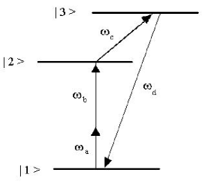
Figure 3: Energy-level diagram of a prototype atomic system for the sum frequency process $\omega_{d}=\omega_{a}+\omega_{b}+\omega_{c}$.

It can be shown [108] that when the field at $\omega_{c}$ is applied, the $\chi^{(3)}$ medium becomes transparent to the resonant transition $|1\rangle\rightarrow|3\rangle$, while in the absence of $\omega_{c}$ the radiation at $\omega_{d}$ is strongly absorbed. The transparency is due to the destructive interference of the two possible absorption transitions $|1\rangle\rightarrow|3\rangle$ and $|2\rangle\rightarrow|3\rangle$. Exploiting EIT can provide large third- or higher-order nonlinear susceptibilities and a minimization of absorption losses. Several proposals, based on the three-level $\Lambda$ configuration as in Fig. (3), or on generalized multi-level schemes, have been made for the enhancement of the Kerr nonlinearity, that shall be discussed in the next Section [111, 112, 113]. Several successful experimental realizations based on the transparency effect have been achieved; for instance, high conversion efficiencies in second harmonic [114] and sum-frequency generation [115] have been obtained in atomic hydrogen, and the experimental observation of large Kerr nonlinearity with vanishing linear susceptibilities has been observed in four-level rubidium atoms [116]. In order to give an idea of the efforts in the direction of producing higher-order nonlinearities of appreciable magnitude, we also mention the proposal of resonant enhancement of $\chi^{(5)}$, based on the effect of coherent population trapping [117].

3.4 Phase matching techniques and experimental implementations

The phase matching condition (83), that is the vanishing of the phase mismatch $\Delta\vec{k}$, is an essential ingredient for the realization of effective, Hamiltonian nonlinear parametric processes. For this reason, we briefly discuss here the most used techniques and some experimental realizations of phase matching. In the three-wave interaction the phase matching condition writes

$$\omega_{a}n_{a}\hat{\imath}_{a}=\omega_{b}n_{b}\hat{\imath}_{b}+\omega_{c}n_{c}\hat{\imath}_{c}\;,$$ (109)

where $n_{q}=n(\omega_{q})$ and $\hat{\imath}_{q}=\vec{k}_{q}/|\vec{k}_{q}|$, $(q=a,b,c)$. For normal dispersion, i.e. $n_{a}>\{n_{b}\,,n_{c}\}$, relation (109) can never be fulfilled. In the process of collinear sum-frequency generation $(\hat{\imath}_{a}=\hat{\imath}_{b}=\hat{\imath}_{c})$, described quantum-mechanically by the Hamiltonian (86), the intensity of the wave $a$ can be computed in the slowly-varying amplitude approximation and is of the form [62]

$$I_{a}\propto\frac{\sin^{2}(\Delta kL)}{(\Delta kL)^{2}}\,,$$ (110)

where $L$ is the effective path length of the light propagating through the crystal. The phase mismatch defines a coherence length $L_{coh}=1/\Delta k$, which must be sufficiently long in order to allow the sum-frequency process. Commonly, in optically anisotropic crystals, phase matching is achieved by exploiting the birefringence, i.e. the dependence of the refractive index on the direction of polarization of the optical field. In 1962, by exploiting the birefringence and the dispersive properties of the crystal, Giordmaine [118] and Maker et al. [119] independently observed second harmonic generation in potassium dihydrogen phosphate. The relation (110) was experimentally verified by Maker et al [119]. In order to illustrate the phenomenon of birefringence in brief, let us consider the class of uniaxial crystals (trigonal, tetragonal, hexagonal). Ordinary polarized light (with polarization orthogonal to the plane containing $\vec{k}$ and the optical axis) undergoes ordinary refraction with index $n^{ord}$; extraordinary polarized light (with polarization parallel to the plane containing $\vec{k}$ and the optical axis) experiences refraction with the extraordinary refractive index $n^{ext}$; the latter depends on the angle $\theta$ between $\vec{k}$ and the optical axis; if they are orthogonal, the ordinary and extraordinary refraction indices coincide to the same value $n_{o}$, and when they are parallel, the extraordinary refraction index assumes its maximum value $n_{e}$ (obviously both $n_{o}$ and $n_{e}$ depend on the material). For generic angles, we have

$$n^{ord}\equiv n_{o}\,,\quad n^{ext}(\theta)=\frac{n_{o}n_{e}}{(n_{e}^{2}\sin^{2}\theta+n_{o}^{2}\cos^{2}\theta)^{1/2}}\;,$$ (111)

where the values of $n_{o}$ and $n_{e}$ are known at each frequency. In Fig. (4), the scheme represents the experimental setup for second harmonic generation by angle-tuned phase matching.

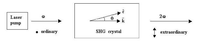
Figure 4: Type I second harmonic generation in negative uniaxial crystal. $\hat{c}$ is the optic axis. The process is phase matched if $n^{ext}(2\omega,\theta)=n^{ord}(\omega)$.

In a series of papers, Midwinter and Warner [120, 121] analyzed and classified the phase matching techniques for three- and four-wave interactions in uniaxial crystals. Tables 1 and 2 summarize the possible phase matching methods for positive and negative uniaxial crystals, i.e., respectively, uniaxial crystals with $(n_{e}>n_{o})$ and $(n_{e}<n_{o})$.

	Positive uniaxial	Negative uniaxial
	$(n_{e}>n_{o})$	$(n_{e}<n_{o})$
Type I	$n_{a}^{ord}\omega_{a}=n_{b}^{ext}\omega_{b}+n_{c}^{ext}\omega_{c}$	$n_{a}^{ext}\omega_{a}=n_{b}^{ord}\omega_{b}+n_{c}^{ord}\omega_{c}$
Type II	$n_{a}^{ord}\omega_{a}=n_{b}^{ord}\omega_{b}+n_{c}^{ext}\omega_{c}$	$n_{a}^{ext}\omega_{a}=n_{b}^{ext}\omega_{b}+n_{c}^{ord}\omega_{c}$

Table 1: Phase matching methods for three-wave interaction in uniaxial crystals.

	Positive uniaxial	Negative uniaxial
Type I	$n_{4}^{ord}\omega_{4}=n_{3}^{ext}\omega_{3}+n_{2}^{ext}\omega_{2}+n_{1}^{ext}\omega_{1}$	$n_{4}^{ext}\omega_{4}=n_{3}^{ord}\omega_{3}+n_{2}^{ord}\omega_{2}+n_{1}^{ord}\omega_{1}$
Type II	$n_{4}^{ord}\omega_{4}=n_{3}^{ext}\omega_{3}+n_{2}^{ext}\omega_{2}+n_{1}^{ord}\omega_{1}$	$n_{4}^{ext}\omega_{4}=n_{3}^{ord}\omega_{3}+n_{2}^{ord}\omega_{2}+n_{1}^{ext}\omega_{1}$
Type III	$n_{4}^{ord}\omega_{4}=n_{3}^{ext}\omega_{3}+n_{2}^{ord}\omega_{2}+n_{1}^{ord}\omega_{1}$	$n_{4}^{ext}\omega_{4}=n_{3}^{ord}\omega_{3}+n_{2}^{ext}\omega_{2}+n_{1}^{ext}\omega_{1}$

Table 2: Phase matching methods for four-wave interaction in uniaxial crystals.

Concerning more complex configurations, we should mention phase-matched three-wave interactions in biaxial crystals discussed in Refs. [122, 123] and phase matching via optical activity, first proposed by Rabin and Bey [124], and successively further investigated by Murray et al. [125].

In order to circumvent the difficulties in realizing exact phase matching, for instance when trying to realize concurrent interactions or in those frequency ranges where it does not hold, one can resort to the technique of so-called quasi phase matching. This idea was introduced in a seminal work on media with periodic modulation of the nonlinearity by Armstrong et al. [126], already in 1962; the same approach was proposed by Franken and Ward [127] one year later. Media with periodic modulation of the nonlinearity consist of a repeated chain of elementary blocks, where in each block of charachteristic linear dimension $\Lambda$ the susceptibility takes opposite signs in each of the two halves of the block. This kind of structure allows for a quasi phase matching condition in the sense that the destructive interference caused by dispersive propagation is compensated by the inversion of the sign of the nonlinear susceptibility. As an example, Fig. (5) represents a scheme for second harmonic generation exploiting collinear quasi phase matching in a periodically poled nonlinear crystal.

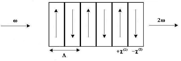
Figure 5: Quasi phase matching for the second harmonic generation in a periodically poled nonlinear crystal. $\Lambda$ is the period of modulation of the susceptibility $\chi^{(2)}$.

When the quasi phase matching condition

$$k(2\omega)-2k(\omega)=\frac{2\pi}{\Lambda}$$ (112)

is satisfied, then the oscillating factor appearing in the integral in Eq.(84) is of order one, guaranteeing the non vanishing of the effective interaction much in the same way as exact phase matching. This technique has been applied to several materials, as $LiNbO_{3}$, $KTP$, $LiTaO_{3}$, fibres, polymers, and semiconductors (see, e.g. Refs. [128]). Being applicable to a very large class of material media, the methods of quasi phase matching help to use very high nonlinear coefficients, otherwise not accessible with the standard techniques based on birefringence. Finally, we wish to mention that quasi phase-matching conditions have been recently realized in quasi-periodic optical superlattices in order to generate second [129] and third harmonic [130].

4 Second and third order optical parametric processes

Moving on from the basic aspects introduced in Section 3, we now begin to discuss in some detail the most important multiphoton processes occurring in nonlinear media. In this Section we restrict the analysis to processes generated by the strongest optical nonlinearities, i.e. those associated to the second- and third-order susceptibilities as described by the trilinear Hamiltonian (86) and the quadrilinear Hamiltonian (89). Historically, after the experimental generation of the second harmonic of the laser light [59], the first proposal for a quantum-mechanical model of the frequency amplifier and frequency converter was presented by Louisell, Yariv, and Siegman [131]. Several papers dedicated to the analysis of the statistical properties of these models rapidly followed [132, 133, 134]. Frequency down conversion was observed for the first time in 1970, in photon coincidence counting experiments [135], and successively it was observed in time-resolved correlation measurements [136]. Models based on four-wave interactions were considered by Yuen and Shapiro [137] and Yurke [138], and in the 1980’s several experiments using four-wave mixing in nonlinear media were reported (See e.g. [139, 140, 141]. Finally, we need to recall that detailed analysis of the three- and four-wave interactions was given by Armstrong et al. [126], who discussed and found the exact solutions for the classical coupled equations. In the following we give an overview on the quantum models and quantum states associated with three- and four-wave interactions, as well as the exact and approximate mathematical methods to study the corresponding dynamics. We will also recall some important experimental realizations and proposals.

The lowest order nonlinearity $\chi^{(2)}$ is responsible of three-photon processes whose dynamics is governed by Hamiltonians of the form (86), which, in the pure quantum case, can be exactly solved only by numerics (See below for more details). Most theoretical analyses have thus been concerned with physical situations such that one mode, the pump mode, is highly excited and can be considered in a high-amplitude coherent state. In such a case, we can resort to the so-called parametric approximation: the pump mode is treated classically as a $c$-number, thus neglecting the depletion mechanism and the quantum fluctuations. Consequently, for instance, bilinear and trilinear models are greatly simplified and reduce, respectively, to linear and bilinear ones. This fact allows exact solvability by the application of standard methods like the disentangling formulas for Lie algebras. The range of validity of the parametric approximation has been investigated in Ref. [142, 143, 144, 145, 146]. In particular, D’Ariano et al. have shown that the usual requirements, i.e. short interaction time and strong classical undepleted pump are too restrictive, and that the main requirement is only that the pump remains coherent after interaction with the medium has occurred [146].

4.1 Three-wave mixing and the trilinear Hamiltonian

The fully quantized, lowest order multiphoton process is described by the trilinear Hamiltonian

$$H^{trl}\;=\;H_{0}+H_{mix}^{3wv}\;=\;\omega_{a}a^{{\dagger}}a+\omega_{b}b^{{\dagger}}b+\omega_{c}c^{{\dagger}}c+\kappa^{(2)}(a^{{\dagger}}bc+ab^{{\dagger}}c^{{\dagger}})\;,$$ (113)

where $\omega_{a}=\omega_{b}+\omega_{c}$, and the coupling constant $\kappa^{(2)}$ is assumed to be real. The Hamiltonian (113) describes the two-photon down-conversion process in the crystal (one photon of frequency $\omega_{a}$ is absorbed, and two photons of frequencies $\omega_{b},\omega_{c}$ are emitted), and the sum-frequency generation (two photons of frequencies $\omega_{b},\omega_{c}$ are absorbed and one photon of frequency $\omega_{a}$ is emitted). Several aspects of model (113) have been thoroughly studied in the literature [143, 147, 148, 149, 150, 151, 152, 153, 154, 155, 156, 157, 158, 159, 160, 161]. The first description of the parametric amplifier and frequency converter, without the classical approximation for the pumping field, was performed by Walls and Barakat [147], who solved exactly the quantum-mechanical problem by the technique of the integrals of motion. In the following we briefly outline this method [147], considered also by other authors [155, 156, 160, 161], by applying it to the case of parametric amplification, with $a$ denoting the laser mode, $b$ the idler mode, and $c$ the signal mode. The system (113) possesses five integrals of motion, with three of them being independent. The five invariants are the operators $H_{0}$, $H_{mix}^{3wv}$, $N_{ab}=a^{{\dagger}}a+b^{{\dagger}}b$, $N_{ac}=a^{{\dagger}}a+c^{{\dagger}}c$, and $D_{bc}\equiv N_{ac}-N_{ab}=c^{{\dagger}}c-b^{{\dagger}}b$, the last three being known as Manley-Rowe invariants [162]. Having three independent integrals of motion, the system can be characterized by three independent quantum numbers. Exploiting such numbers, the dynamics of the system can be studied by decomposing the Hilbert space $\mathcal{H}$ associated with Hamiltonian (113) in a direct sum of finite-dimensional subspaces. Let us then choose as independent conserved quantities the operators $N_{ab}$, $D_{bc}$, and $H_{mix}^{3wv}$, let us fix the (integer) eigenvalues $N$ of $N_{ab}$, and $D$ of $D_{bc}$, and let us finally write down the eigenvalue equations in this subspace $\mathcal{H}_{N,D}$ of fixed $N$ and $D$:

$$N_{ab}|\lambda_{j}(N,D)\rangle=N|\lambda_{j}(N,D)\rangle\;,\quad D_{bc}|\lambda_{j}(N,D)\rangle=D|\lambda_{j}(N,D)\rangle\;,$$ (114)

$$H_{mix}^{3wv}|\lambda_{j}(N,D)\rangle=\lambda_{j}(N,D)|\lambda_{j}(N,D)\rangle\;.$$ (115)

For fixed values of $N$ and $D$, the eigenvalues $\lambda_{j}(N,D)$ of $H_{mix}^{3wv}$ and the common eigenvectors $|\lambda_{j}(N,D)\rangle$ are obtained by diagonalizing $H_{mix}^{3wv}$ on the subspace $\mathcal{H}_{N,D}$. The latter is spanned by the set of vectors of the form $\{|n\rangle_{N,D}=|N-n\rangle_{a}|n\rangle_{b}|D+n\rangle_{c}\,,0\leq n\leq N\}$, where $|n\rangle_{a}|m\rangle_{b}|l\rangle_{c}$ are the three-mode number states. In this basis, the matrix representation of $H_{mix}^{3wv}$ is

$$H_{mix}^{3wv}\;=\;\kappa^{(2)}\left(\begin{array}[]{ccccccc}0&h_{0}&0&0&0&\cdots&0\\ h_{0}&0&h_{1}&0&0&\cdots&0\\ 0&h_{1}&0&h_{2}&0&\cdots&0\\ 0&0&h_{2}&0&h_{3}&\cdots&0\\ \vdots&\vdots&\ddots&\ddots&\ddots&\ddots&h_{N-1}\\ 0&\cdots&\cdots&\cdots&0&h_{N-1}&0\\ \end{array}\right)\,;$$ (116)

where $h_{r}=\sqrt{(N-r)(D+r+1)(r+1)}$, $(0\leq r\leq N-1)$. The final form of the eigenvalue equation for $H^{trl}$ can be written as:

$$H^{trl}|\lambda_{j}(N,D)\rangle = [(\omega_{a}N_{ab}+\omega_{c}D_{bc})+H_{mix}^{3wv}]|\lambda_{j}(N,D)\rangle$$ (117)

$$= [\omega_{a}N+\omega_{c}D+\lambda_{j}(N,D)]|\lambda_{j}(N,D)\rangle\;.$$

The eigenvectors $|\lambda_{j}(N,D)\rangle$ in the subspace, can be expressed as superpositions of the number-state basis vectors, $|\lambda_{j}(N,D)\rangle=\sum_{i=0}^{n}u_{ji}(N,D)|n\rangle_{N,D}$, where the values of $u_{ji}(N,D)$ have to be determined numerically. Therefore, fixed finite values of $N$ and $D$, the dynamics can be solved exactly, albeit numerically, by determining the eigenvalues $\lambda_{j}(N,D)$ and the orthonormal eigenvectors $|\lambda_{j}(N,D)\rangle$ of the $(N+1)\times(N+1)$ matrix (116). Clearly, the dynamics depends crucially on the nature of the initial state. Typical choices are three-mode number states (for their simplicity), and states of the coherent form $|\alpha\rangle|0\rangle|0\rangle$ that represent the initial condition for spontaneous parametric down conversion (here $|\alpha\rangle$ denotes the coherent state for the pump mode). This technique has been exploited to study the statistics and the squeezing properties of the signal mode [155], and the time evolution of the entanglement between the modes [156]. The system can exhibit sub-Poissonian statistics and anticorrelation (roughly speaking, two-mode antibunching as measured by the cross-correlation function), as well as strong entanglement between the pump and signal or idler modes. Moreover, the model is characterized by the appearance of collapses and revivals in the mean photon numbers [147, 155].
Analytic solutions of the dynamics generated by the Hamiltonian (113) can be accomplished under short-time approximations, which are however realistic due to the usually very short interaction times [148, 149, 160]. The nonlinear, coupled dynamical equations

$$i\frac{da(t)}{dt}=\omega_{a}a(t)+\kappa^{(2)}b(t)c(t)\;,$$

$$i\frac{db(t)}{dt}=\omega_{b}b(t)+\kappa^{(2)}a(t)c^{{\dagger}}(t)\;,$$

$$i\frac{dc(t)}{dt}=\omega_{c}c(t)+\kappa^{(2)}a(t)b^{{\dagger}}(t)\;,$$ (118)

can be solved by expanding each mode in a Taylor series up to quadratic terms and by exploiting the equations of motion; for instance, the time evolution of the signal mode operator $c$, up to second order in the dimensionless reduced time $\kappa^{(2)}t$, is given by

$$c(t)\;=\;c\,-\,i\kappa^{(2)}tb^{{\dagger}}a\,+\,\frac{(\kappa^{(2)}t)^{2}}{2!}c(a^{{\dagger}}a\,-\,b^{{\dagger}}b)\,+\,\mathcal{O}[(\kappa^{(2)}t)^{3}]\;,$$ (119)

where $a$, $b$, $c$ in the right hand side of Eq. (119) denote the initial values of the operators at time $t=0$. Given Eq. (119), the dynamics of the signal mode $c$ is determined, for example by resorting to its diagonal coherent state representation [148].
Another interesting method [151] to obtain analytic solutions for three-wave mixing is based on the use of generalized Bose operators introduced by Brandt and Greenberg [163], and put in a closed form by Rasetti [164]. Let us define the pair of operators [151]

$$A=F(n_{b},n_{c})bc\;,\quad\quad A^{{\dagger}}=c^{{\dagger}}b^{{\dagger}}F^{*}(n_{b},n_{c})\;,$$ (120)

where $F(n_{b},n_{c})$ is an operatorial function of the number operators for modes $b$ and $c$, that is fixed by imposing the bosonic canonical commutation relation $[A,A^{{\dagger}}]=1$. It can then be shown that $|F(n_{b},n_{c})|^{2}(n_{b}+1)(n_{c}+1)-|F(n_{b}-1,n_{c}-1)|^{2}n_{b}n_{c}=1$, and by induction that $|F(n_{b},n_{c})|^{2}=(n_{>}+1)^{-1}$ with $n_{>}=\max\{n_{b},n_{c}\}$. As $D_{bc}\equiv n_{c}-n_{b}$ is a constant of the motion, under the hypothesis that the mode $c$ is much more intense than the mode $b$, we can write $b^{{\dagger}}b\simeq A^{{\dagger}}A$ and $c^{{\dagger}}c\simeq n_{0}+A^{{\dagger}}A$, where $n_{0}$, the difference in the number of photons in the two modes, satisfies $n_{0}\gg 1$. The Hamiltonian (113) can then be expressed in the form

$$H^{trl}\, = \,\omega_{c}n_{0}+\omega_{a}(A^{{\dagger}}A+a^{{\dagger}}a)$$ (121)

$$+\kappa^{(2)}\left[a^{{\dagger}}\frac{1}{F(n_{b},n_{c})}A+A^{{\dagger}}\frac{1}{F^{*}(n_{b},n_{c})}a\right].$$

Under the imposed condition $n_{0}\gg 1$, $F$ can be treated as a constant and $H^{trl}$ reduces to

$$\tilde{H}^{trl}=\omega_{a}(A^{{\dagger}}A+a^{{\dagger}}a)+\tilde{\kappa}^{(2)}(a^{{\dagger}}A+A^{{\dagger}}a)\;,$$ (122)

where $\tilde{\kappa}^{(2)}=\kappa^{(2)}/F\simeq\kappa^{(2)}/\sqrt{n_{0}}$, and the constant term $\omega_{c}n_{0}$ has been dropped. The solution of the Heisenberg equation of motion for mode $a$ is

$$a(t)=e^{-i\omega_{a}t}[a\cos(\tilde{\kappa}^{(2)}t)-iA\sin(\tilde{\kappa}^{(2)}t)]\;,$$ (123)

where in the r.h.s $a$ and $A$ are the initial-time operators. Therefore, the mean number of photons in mode $a$, taking an initial two-mode Fock number state $|n_{b},n_{c}\rangle$, is $\langle n_{a}(t)\rangle=\sin^{2}(\tilde{\kappa}^{(2)}t)n_{<}$, where $n_{<}$ denotes the mean number of photons in the less intense between the modes $b$ and $c$. The number of photons in mode $a$ hence exhibits oscillations with period $\pi/\tilde{\kappa}^{(2)}$, in close agreement with the result of Walls and Barakat [147].
Other approaches have been used to analyze the dynamics of the system (113): Jurčo found exact solutions using the Bethe ansatz [153]; Gambini and Carusotto solved the coupled nonlinear equations of motion by using iteration methods [149, 154]; McNeil and Gardiner have studied the process in a cavity by finding the solution of a Fokker-Planck equation [152]; Hillery et al. determined exact relations between the number fluctuations of the three modes [158].
With the particular choice $\omega_{b}=\omega_{c}=\omega_{a}/2$ [155, 161], the Hamiltonian (113) can be expressed in the form

$$H^{trl}_{su11}=\omega_{a}(a^{{\dagger}}a+K_{0})+\kappa^{(2)}(aK_{+}+a^{{\dagger}}K_{-})\;,$$ (124)

where the operators

$$K_{+}=b^{{\dagger}}c^{{\dagger}}\;,K_{-}=bc\;,K_{0}=\frac{1}{2}(b^{{\dagger}}b+c^{{\dagger}}c+1)\;,$$ (125)

span the $SU(1,1)$ Lie algebra:

$$[K_{0},K_{\pm}]=\pm K_{\pm}\;,\quad[K_{-},K_{+}]=2K_{0}\;.$$ (126)

Clearly, the form (124) is suitable for the description of interactions with underlying $SU(1,1)$ symmetry, such as parametric amplification. The Casimir operator

$$C=K_{0}^{2}-\frac{1}{2}(K_{+}K_{-}+K_{-}K_{+})=\frac{1}{4}(D_{bc}^{2}-1)=k(k-1)\;,$$ (127)

is an invariant of the motion. The Bargmann index $k=\frac{1}{2}(|D_{bc}|+1)$ takes the discrete values $k=\frac{1}{2},1,\frac{3}{2},2,...$ [165]. Given the quantum number $L=N_{ac}$, the diagonalization method proceeds along lines similar to those of Walls and Barakat that we have already illustrated: the whole Hilbert space can be decomposed into a direct sum of finite-dimensional subspaces $\mathcal{H}_{L}$. Each subspace is spanned by the complete orthonormal set $\{|n\rangle_{a}|k,L-n\rangle,\;n=0,...,L\}$, where $|k,m\rangle$ denotes the two-mode Fock number state of the following form $|m+2k-1\rangle_{b}|m\rangle_{c}$. A set of generalized coherent states associated with the Hamiltonian (124) has also been introduced [161]:

$$|z;k,L\rangle=\mathcal{N}^{-1/2}e^{zaK_{+}}|L\rangle_{a}|k,0\rangle\;,$$ (128)

where $z=-i\kappa^{(2)}t$ and $|L\rangle_{a}|k,0\rangle$ is the initial reference state. It can be shown that the system evolves from the reference state into the coherent state (128) during the very early stage of the dynamics with respect to $1/\kappa^{(2)}$.
For $b=c$, the $SU(1,1)$ operators read:

$$K_{+}=\frac{1}{2}b^{{\dagger}2}\;,K_{-}=\frac{1}{2}b^{2}\;,K_{0}=\frac{1}{2}\left(b^{{\dagger}}b+\frac{1}{2}\right)\;,$$ (129)

and $k=\frac{1}{4}$ or $\frac{3}{4}$. The dynamics induced by the corresponding, fully quantized Hamiltonian, gives rise to degenerate parametric amplification or second harmonic generation, and has been studied in detail in Refs. [142, 144, 166, 167, 168, 169, 170].

4.2 Four-wave mixing and the quadrilinear Hamiltonians

We now move on to discuss four-photon processes and four-wave mixing, that is the parametric interaction between four photons in third-order nonlinear media. After introducing the fundamental aspects, we will focus on the most recent theoretical and experimental progresses. The naming “Four-wave mixing” stands for many different types of interactions that can all be described by Hamiltonian terms of the general form (89). Taking into account also the free Hamiltonian part, we can rewrite the total Hamiltonians, comprising the free and the interaction parts, for the two different types of four-wave mixing as follows, with obvious meaning of the notations:

$$H_{Tj}^{4wm}\;=\;H_{0}^{4wm}\,+\,H_{Ij}^{4wm}\;,\;\quad(j=1,2)\;,$$ (130)

$$H_{0}^{4wm}\;=\;\sum_{q}\omega_{q}q^{{\dagger}}q\;,\;\quad(q=a,b,c,d)\;,$$ (131)

$$H_{I1}^{4wm}\;=\;\kappa_{1}^{(3)}a^{{\dagger}}b^{{\dagger}}c^{{\dagger}}d+\kappa_{1}^{(3)*}abcd^{{\dagger}}\;\;,\quad\omega_{a}+\omega_{b}+\omega_{c}=\omega_{d}$$ (132)

$$H_{I2}^{4wm}\;=\;\kappa_{2}^{(3)}a^{{\dagger}}b^{{\dagger}}cd+\kappa_{2}^{(3)*}abc^{{\dagger}}d^{{\dagger}}\;\;,\quad\omega_{a}+\omega_{b}=\omega_{c}+\omega_{d}\;,$$ (133)

where $a$, $b$, $c$, $d$ are four distinct quantum modes, and the complex couplings $\kappa_{j}^{(3)}$ $(j=1,2)$ are proportional to the third order susceptibilities. The sum-rule conditions on the frequencies are due to energy conservation, and the corresponding phase matching conditions have been tacitly assumed.

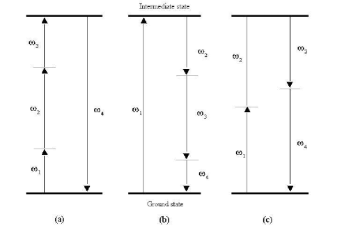
Figure 6: Schematic description of quantum transitions for general nondegenerate four-wave mixing processes: (a) sum-frequency generation, (b) three-photon down conversion, (c) two-photon down conversion from two pumping waves.

In Fig. (6) we report some typical schemes for quantum parametric transitions associated to the most important four-wave mixing interactions. In a parametric process, the medium, initially in its ground state, reaches, due to the interaction with the radiation field, an intermediate, excited state, and then finally decays back to the ground state. Each process is characterized by different input and output frequency combinations, consistent with the physical matching conditions. Fig. (6) (a) and (b), corresponding to the Hamiltonian (132), represent, respectively, the sum-frequency process and the three-photon down conversion process. Fig. (6) (c), corresponding to the Hamiltonian (133), refers to the interaction event in which two input photons are annihilated with the consequent creation of the signal and idler photons in the nonlinear medium. It is evident that the degeneracy of two or more modes in Eqs. (132) and (133) leads to a large subclass of models, such as Kerr or cross-Kerr interaction and degenerate three-photon down conversion process. Moreover, the single or repeated application of the parametric approximation (high-intensity coherent regime) for the pump modes can simplify the Hamiltonians, reducing them to trilinear or bilinear forms. Four-wave mixing was first proposed by Yuen and Shapiro for the generation of squeezed light [137]; they considered the so-called backward configuration in which both the two pump fields and the two signal fields are counterpropagating. Successively, Yurke proposed the generation of squeezed states by means of four-wave mixing in an optical cavity [138]. A fully quantum-mechanical theory of nondegenerate mixing in an optical cavity containing a nonlinear medium of two-level atoms was introduced by Reid and Walls [171]. The first experimental observations of squeezed light by means of four-wave mixing are due to Bondurant et al. [139], Levenson et al. [140], Slusher et al. [141]. Since these successful experimental realizations, great attention has been dedicated to the study of the quantum statistics of this process: a review and a bibliographic guide can be found in Ref. [172]. One should remark the importance of four-wave mixing as a tool for nonlinear spectroscopy, due to the enhancement of the process occurring at the resonances characteristic of the medium; see for instance [173, 174].
As already seen for three-wave mixing, exact treatments of the dynamics of the interaction models (132) and (133) are possible only in a numerical framework. Analytical results can be obtained in some approximation schemes. For instance, in the short-time approximation [175], one can investigate the squeezing power of the four-wave interaction $H_{I2a}^{4wm}=\kappa(a^{{\dagger}2}cd+a^{2}c^{{\dagger}}d^{{\dagger}})$, that is, the model (133) with a single pump $(a=b)$ and $2\omega_{a}=\omega_{c}+\omega_{d}$. Alternatively, the four-wave interactions (132) and (133) can be linearized by using a specific form of the generalized Bose operators, already introduced for trilinear Hamiltonians in the previous Subsection [151]. In this approach, one can derive integral equations for the time evolution of the photon number operators, that are solvable in terms of Jacobian elliptic functions.
It is important to discuss in some detail recent theoretical and experimental results related to the question of possible large enhancement of four-wave mixing. This can be obtained by an ingenious application of electromagnetically induced transparency (EIT, see also the previous Section) to suppress the single- and multi-photon absorption that limits the efficiency of third-order processes. In the last years, different schemes of four-wave mixing enhancement have been proposed, based on $\Lambda$ and double-$\Lambda$ transitions. [176, 177, 178, 179, 180]. Here we review a method due to Johnsson and Fleischauer for the realization of resonant, forward four-wave mixing [177, 178]. These authors have considered the double-$\Lambda$ configuration depicted in Fig. (7); it represents a symmetric five-level setup $(|0\rangle\,,|1\rangle\,,|2\rangle\,,|3\rangle\,,|4\rangle)$, which is particularly convenient because in this configuration the ac-Stark shifts, that reduce the conversion efficiency, are cancelled.

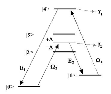
Figure 7: Double-$\Lambda$ transition scheme. $\Omega_{j}$ $(j=1,2)$ represent the pump fields, $E_{j}$ $(j=1,2)$ represent the signal and the idler fields, and $|0\rangle$ and $|1\rangle$ are two metastable ground states. The scheme allows the cancellation of destructive phase shifts.

Here $\Omega_{j}$ $(j=1,2)$ denote the driving fields, with $\Omega_{1}$ assumed to be in resonance with the $|1\rangle\rightarrow|4\rangle$ transition, i.e. $\omega_{\Omega_{1}}=\omega_{41}$, while $\Omega_{2}$ has a detuning $\Delta$, i.e. $\omega_{\Omega_{2}}=\omega_{30}-\Delta=\omega_{20}+\Delta$. The $E_{j}$s are the signal and idler fields with $E_{1}$ assumed to be in resonance with the $|4\rangle\rightarrow|0\rangle$ transition, i.e. $\omega_{E_{1}}=\omega_{40}$, while $E_{2}$ has a detuning $\Delta$, i.e. $\omega_{E_{2}}=\omega_{31}-\Delta=\omega_{21}+\Delta$. The finite detuning $\Delta$ is assumed to be large compared to the Rabi frequencies in order to ensure the minimization of linear losses due to single-photon absorption. Moreover, it is assumed that the pump and the generated fields, propagating in the same direction $z$, are pairwise in two-photon resonance, and thus, globally, in four-photon resonance, i.e. $\omega_{\Omega_{1}}+\omega_{\Omega_{2}}=\omega_{E_{1}}+\omega_{E_{2}}$. One can thus proceed first to derive an effective classical interaction Hamiltonian in the adiabatic limit, and then to quantize it [177]. The effective non Hermitian interaction Hamiltonian, in a rotating wave approximation corresponding to slowly varying amplitudes of the basis $(|0\rangle\,,|1\rangle\,,|2\rangle\,,|3\rangle\,,|4\rangle)^{T}$, can be written in the following form:

$$H_{I}=-\left(\begin{array}[]{ccccc}0&0&\Omega_{2}^{*}&\Omega_{2}^{*}&E_{1}^{*}\\ 0&0&E_{2}^{*}&-E_{2}^{*}&\Omega_{1}^{*}\\ \Omega_{2}&E_{2}&-\Delta+i\gamma_{2}&0&0\\ \Omega_{2}&-E_{2}&0&\Delta+i\gamma_{2}&0\\ E_{1}&\Omega_{1}&0&0&i\gamma_{1}\end{array}\right)\;.$$ (134)

At the input the signal and the idler fields are assumed to have zero amplitudes, and all atoms are in the ground state $|0\rangle$. This state results to be an approximate adiabatic eigenstate of $H_{I}$, which can then be replaced by the corresponding eigenvalue. Solving the characteristic equations for the eigenvalues, and expanding the ground-state one in a power series to the lowest order in $\Delta^{-1}$, one obtains

$$H_{I}=\frac{1}{\Delta}\left(\frac{\Omega_{1}^{*}\Omega_{2}^{*}E_{1}E_{2}+\Omega_{1}\Omega_{2}E_{1}^{*}E_{2}^{*}}{|\Omega_{1}|^{2}+|E_{1}|^{2}}\right)\;.$$ (135)

Here we see EIT at work: as a consequence of the quantum interference leading to the induced transparency, the resonant interaction has no imaginary component left, and therefore there is no linear loss. The quantization of $H_{I}$ is achieved by replacing the complex amplitudes by the corresponding positive and negative operators in normal ordered form, and by inserting the density of atoms $N$, the effective cross section of the beams $A$, and by integrating over the interaction volume. The effective interaction Hamiltonian then reads [177]

$$H_{I}=\frac{NA}{\Delta}\int dz\left(\frac{\Omega_{1}^{{\dagger}}\Omega_{2}^{{\dagger}}E_{1}E_{2}+\Omega_{1}\Omega_{2}E_{1}^{{\dagger}}E_{2}^{{\dagger}}}{\Omega_{1}^{{\dagger}}\Omega_{1}+E_{1}^{{\dagger}}E_{1}}\right)\;.$$ (136)

It is possible to verify that there are four independent constants of motion $(\Omega_{1}^{{\dagger}}\Omega_{1}+E_{1}^{{\dagger}}E_{1})$, $(\Omega_{2}^{{\dagger}}\Omega_{2}+E_{2}^{{\dagger}}E_{2})$, $(\Omega_{1}^{{\dagger}}\Omega_{1}-\Omega_{2}^{{\dagger}}\Omega_{2})$, and $(\Omega_{1}^{{\dagger}}\Omega_{2}^{{\dagger}}E_{1}E_{2}+\Omega_{1}\Omega_{2}E_{1}^{{\dagger}}E_{2}^{{\dagger}})$. By exploiting them under stationary conditions, the dynamics of the system has been analyzed numerically up to $10^{3}$ input photons [177]. An oscillatory exchange between the modes has been observed both for initial number states and for initial coherent states; moreover, the statistics turned out to be superPoissonian in most of the time regimes. The possible application of this setup for the realization of a photonic phase gate has also been studied [177, 178], and will be discussed in more detail in Section (7) together with other proposed applications of four-wave mixing interactions to entanglement generation, quantum information protocols, and quantum gates for quantum computation. Remarkably, experimental demonstrations of four-wave mixing using the EIT effect have been recently realized in systems of ultracold atoms [181, 182]. In the experiment described in Ref. [181] backward four-wave mixing with EIT is obtained in a double-$\Lambda$ system engineered by four levels of increasing energy, $|0\rangle,|1\rangle,|2\rangle,|3\rangle$, of ultracold atoms of $\,{}^{87}Rb$. A coupling laser of frequency $\omega_{c}$, tuned to the transition $|1\rangle\rightarrow|2\rangle$ between the intermediate energy states, sets up a quantum interference, and provides EIT for an anti-Stokes laser of frequency $\omega_{AS}$. The anti-Stokes laser is tuned to the transition $|2\rangle\rightarrow|0\rangle$, and a pump laser of frequency $\omega_{p}$ is detuned from the $|0\rangle\rightarrow|3\rangle$ resonance. If the pump and coupling lasers are strong, and the anti-Stokes laser is weak, the anti-Stokes beam generates a counterpropagating Stokes beam of frequency $\omega_{S}$, that satisfies phase matching, and energy conservation: $\omega_{S}=\omega_{p}+\omega_{c}-\omega_{AS}$. The four-wave mixing process is thus realized, with the anti-Stokes laser producing photons with a nearly $100\%$ transmission at line center of the resonant transition $|2\rangle\rightarrow|0\rangle$; this fact can be of relevance for transmission of quantum information. A similar scheme is realized in Ref. [182].

The time-independent quantum mechanics of four-wave mixing Hamiltonians is of particular interest, because it is possible in certain cases to obtain analytical results for their spectra. In the case of various, fully quantized multiwave-mixing models, the so-called Bethe ansatz is commonly used [183]. Such an approach is based on the assumption that the form of the energy eigenstates can be expressed in terms of several Bethe parameters. However, the equations for these parameters are very complicated even for numerical solution. An alternative, algebraic method has been recently proposed and applied to obtain explicit analytical expressions both for the eigenenergies and the eigenstates of the total Hamiltonians $H_{Tj}^{4wm}$ Eq. (130) [184]. Here we briefly describe this method for the case of the interaction Hamiltonian $H_{I1}^{4wm}$, with $\kappa^{(3)}_{1}$ taken to be real for simplicity. The same procedure can be applied along similar lines to the model with interaction $H_{I2}^{4wm}$. Concerning the total Hamiltonian $H_{T1}^{4wm}$, the following operators are integrals of motion: $N_{ad}=n_{a}+n_{d}$, $N_{bd}=n_{b}+n_{d}$, $N_{cd}=n_{c}+n_{d}$, $H_{0}^{4wm}=\omega_{a}N_{ad}+\omega_{b}N_{bd}+\omega_{c}N_{cd}$, and $H_{I1}^{4wm}$. Therefore, these operators share a complete set of eigenstates $|\Psi_{N_{ad},N_{bd},N_{cd},\lambda}\rangle$ satisfying the relations:

$$H_{T1}^{4wm}|\Psi_{N_{ad},N_{bd},N_{cd},\lambda}\rangle\;=\;E_{N_{ad},N_{bd},N_{cd},\lambda}|\Psi_{N_{ad},N_{bd},N_{cd},\lambda}\rangle\;,$$

$$H^{4wm}_{I1}|\Psi_{N_{ad},N_{bd},N_{cd},\lambda}\rangle\;=\;\lambda|\Psi_{N_{ad},N_{bd},N_{cd},\lambda}\rangle\;,$$

$$E_{N_{ad},N_{bd},N_{cd},\lambda}\;=\;\omega_{a}N_{ad}+\omega_{b}N_{bd}+\omega_{c}N_{cd}+\kappa_{1}^{(3)}\lambda\;,$$

$$N_{ad},N_{bd},N_{cd}=0,1,2,...\;,$$ (137)

where, without danger of confusion, we have used the same symbols for the operators and for the associated quantum numbers. The eigenstates $|\Psi_{N_{ad},N_{bd},N_{cd},\lambda}\rangle$ can be expressed in terms of an operatorial function of the mode creation operators applied to the vacuum, in the form [185]

$$|\Psi_{N_{ad},N_{bd},N_{cd},\lambda}\rangle\;=\;S(a^{{\dagger}},b^{{\dagger}},c^{{\dagger}},d^{{\dagger}})|0,0,0,0\rangle\;,$$

$$S(a^{{\dagger}},b^{{\dagger}},c^{{\dagger}},d^{{\dagger}})\;=\;\sum_{j=0}^{M}\frac{\alpha_{j}}{j!}(a^{{\dagger}})^{N_{ad}-j}(b^{{\dagger}})^{N_{bd}-j}(c^{{\dagger}})^{N_{cd}-j}(d^{{\dagger}})^{j}\;,\;$$

$$M=\min\{N_{ad},N_{bd},N_{cd}\}\;.$$ (138)

As $H_{I1}^{4wm}|\Psi_{N_{ad},N_{bd},N_{cd},\lambda}\rangle=[H_{I1}^{4wm},S]|0,0,0,0\rangle$ it can be shown, using expression (132), that $S$ satisfies the operatorial differential equation

$$\left(d^{{\dagger}}\frac{\partial^{3}}{\partial a^{{\dagger}}b^{{\dagger}}c^{{\dagger}}}+a^{{\dagger}}b^{{\dagger}}c^{{\dagger}}\frac{\partial}{\partial d^{{\dagger}}}\right)S\;=\;\lambda S\;.$$ (139)

Relations (138) and (139) lead to the following recursive equations

$$\alpha_{j+1}\;=\;\lambda\alpha_{j}-p_{j-1}\alpha_{j-1}\;,\;\quad 0\leq j\leq M\;,$$ (140)

where $\alpha_{-1}=\alpha_{M+1}=0$ and $p_{j}=-(j+1)j[(j-1)(j+1-N_{ad}-N_{bd}-N_{cd})+(N_{ad}N_{bd}+N_{bd}N_{cd}+N_{ad}N_{cd}-N_{ad}-N_{bd}-N_{cd}+1)]+(j+1)N_{ad}N_{bd}N_{cd}$. Equation (140) implies

$$\alpha_{j}\;=\;\alpha_{0}\det A^{(j)}(\lambda)\;,\;\quad j=0,1,2,...,M\;,$$ (141)

where $\det A^{(j)}(\lambda)$ is defined as follows: $\det A^{(0)}(\lambda)=1$, $\det A^{(1)}(\lambda)=\lambda$, while for $k\geq 2$ it is the determinant of the $k\times k$ matrix $A^{(k)}(\lambda)$ with elements $A_{ij}^{(k)}(\lambda)=\lambda\delta_{i,j}-\delta_{i+1,j}-p_{j}\delta_{i,j+1}$ $(i,j=0,1,...,k-1)$. The energy eigenvalue $\lambda$ of the interaction part of the Hamiltonian is determined by finding the roots of the polynomial equation

$$\det A^{(M+1)}(\lambda)\;=\;0\;,\;\quad M=\min\{N_{ad},N_{bd},N_{cd}\}\;.$$ (142)

In conclusion, one obtains an analytical expression for the energy spectrum (137) and for the energy eigenstates in terms of the parameter $\lambda$ [184]

$$|\Psi_{N_{ad},N_{bd},N_{cd},\lambda}\rangle\;=\;\sum_{j=0}^{\min\{N_{ad},N_{bd},N_{cd}\}}c_{j}|N_{ad}-j,N_{bd}-j,N_{cd}-j,j\rangle\;,$$ (143)

$$c_{j}\;=\;c_{0}\left[\frac{(N_{ad}-j)!(N_{bd}-j)!(N_{cd}-j)!}{j!N_{ad}!N_{bd}!N_{cd}!}\right]^{1/2}\det A^{(j)}(\lambda)\;,$$ (144)

where $c_{0}$ is a normalization factor and $N_{ad},N_{bd},N_{cd}=M,M+1,...$ $(M=\min\{N_{ad},N_{bd},N_{cd}\})$.

4.3 Two-photon squeezed states by three- and four-wave mixing

Although squeezed states are the simplest example of nonclassical multiphoton states of light, and have thus been extensively investigated both theoretically and experimentally in the literature, here, for completeness, we shall rapidly recall their main properties, and cite some applications and experimental realizations. Extensive treatments on the subject can be found in works [186, 187, 188, 189, 22] and references therein.

Squeezed states can be generated either by considering trilinear interactions with one of the modes in a classical configuration (e.g. intense pump laser $E_{p}$), or by considering quadrilinear (four-wave mixing) interactions with two modes in a classical configuration leading to a classical amplitude $E_{p}^{2}$. In both cases, the Hamiltonian reduces to the quadratic form

$$H_{I}^{2ph}\;=\;\eta^{*}(t)a_{1}a_{2}+\eta(t)a_{1}^{{\dagger}}a_{2}^{{\dagger}}\;,$$ (145)

where, in the trilinear instance the complex parameter $\eta$ is proportional to the $\chi^{(2)}$ nonlinearity and to the coherent pump: $\eta\propto\chi^{(2)}E_{p}$, while, in the quadrilinear case, $\eta\propto\chi^{(3)}E_{p}^{2}$. This approximated Hamiltonian, thoroughly studied in the literature [76, 131, 132, 133, 134, 190, 191, 192, 193, 194], describes the nondegenerate parametric amplifier, whose temporal dynamics generates two-mode squeezed states, which reduce to single-mode squeezed states in the degenerate case $a_{1}=a_{2}\equiv a$. Many experimental schemes for generating squeezed states of light have been proposed, such as the resonance fluorescence [195], the use of free-electron laser [196], the harmonic generation [197], two-photon and multiphoton absorption [198, 199], four-wave mixing [137] and parametric amplification [198, 200].

The first successful experiments on the generation and detection of squeezed states were realized in the 1980s. In 1985, Slusher et al. reported the observation of quadrature squeezing of an optical field by degenerate four-wave mixing in an optical cavity filled with $Na$ atoms [201]. In 1986, Shelby et al. obtained squeezing in an optical fiber via the Kerr effect [202]. In the same year, in a crucial experiment, Wu et al. succeeded in realizing a very large squeezing in parametric down conversion, up to more than $50$ % squeezing in a below-threshold optical parametric oscillator (OPO) [203]. Successively, a number of experiments with analogous results were performed by using both second order [204, 205] and third order nonlinearities [206, 207]. A squeezing ratio of about $70$ % can be currently obtained in silica fibers [208], and in OPOs [209]. It should be noted that noise reduction with respect to classical light can be routinely observed not only in OPOs, i.e. in a continuous-wave oscillator configuration [210], but also in optical parametric amplifiers (OPAs), i.e. in a pulsed amplifier configuration [211]. Number-phase squeezing has been generated as well in diode-laser based devices [212]. Finally, for a comprehensive review of nonlinear quantum optics applied to the control and reduction of quantum noise and the production of squeezed states in artificially phase-matched and quasi phase-matched materials, see Ref. [213].
Historically, squeezed states were originated from the analysis, in the degenerate instance, of unitary and linear Bogoliubov transformations and from the investigation of the possible ways to generate minimum uncertainty states of the radiation field more general than coherent states. The so-called two-photon coherent states of Yuen [186] are based on the Bogoliubov linear transformation $b=\mu a+\nu a^{{\dagger}}$, with $\mu$ and $\nu$ complex parameters that must satisfy the relation $|\mu|^{2}-|\nu|^{2}=1$ for the transformation to be canonical. The transformation $b(a,a^{{\dagger}})$ can also be obtained by action of a unitary operator $S$ on the mode operators: $b(a,a^{{\dagger}})=SaS^{{\dagger}}$. The transformed operators $b$ and $b^{{\dagger}}$ can be interpreted as ”quasi-photon” annihilation and creation operators, and determine a quasi-photon number operator $n_{g}=b^{{\dagger}}b$ with integer positive eigenvalues and a quasi-photon ground state (or squeezed vacuum) $|0_{g}\rangle$ defined by the relation $b|0_{g}\rangle=0$. The quasi-photon number states $|m_{g}\rangle\doteq\frac{b^{{\dagger}m}}{\sqrt{m!}}|0_{g}\rangle\equiv S|m\rangle$ form an orthonormal basis. The two-photon coherent states (TCS) $|\beta\rangle_{g}=|\beta;\mu,\nu\rangle$ are defined as the eigenstates of $b$ with complex eigenvalue $\beta$, such that

$$b|\beta\rangle_{g}\;=\;\beta|\beta\rangle_{g}\;,$$ (146)

and, of course, they reduce to the ordinary coherent states for $\nu=0$. In analogy with the case of the standard one-photon coherent states, the TCS can be expressed as well in terms of the action of a displacement operator depending on the transformed mode variables $(b,b^{{\dagger}})$, i.e.

$$|\beta\rangle_{g}=e^{\beta b^{{\dagger}}-\beta^{*}b}|0_{g}\rangle\equiv S(S^{{\dagger}}e^{\beta b^{{\dagger}}-\beta^{*}b}S)|0\rangle\equiv SD(\beta)|0\rangle\;,$$ (147)

where $D(\beta)=e^{\beta a^{{\dagger}}-\beta^{*}a}$, is the Glauber displacement operator in terms of the original mode variables $(a,a^{{\dagger}})$. The TCS obey non-orthogonality and over-completeness relations similar to those holding for coherent states (14). The condition of canonicity leads to the standard parametrization $\mu=\cosh r\;,\;\nu=e^{i\phi}\sinh r$, and the unitary squeezing operator $S$ can be written in terms of $a$ and $a^{{\dagger}}$ as $S(\varepsilon)=e^{-\frac{1}{2}\varepsilon a^{{\dagger}2}+\frac{1}{2}\varepsilon^{*}a^{2}}$ with $\varepsilon=re^{i\phi}$. Thus, finally, the TCS can be written as $|\beta\rangle_{g}=S(\varepsilon)D(\beta)|0\rangle$. Clearly, it is legitimate to consider switching the order of application of the two unitary operators $D$ and $S$. Doing so, provides an alternative definition that yields in principle a different class of states, the so-called two-photon squeezed states, thus defined as $|\alpha,\varepsilon\rangle=D(\alpha)S(\varepsilon)|0\rangle$, where $D(\alpha)$ is the Glauber displacement operator with generic complex coherent amplitude $\alpha$. However, the two classes of states coincide as soon as one simply lets $\alpha=\mu^{*}\beta-\nu\beta^{*}$. With this identification, in the following, without ambiguity, we will always refer to both classes of states as two-photon squeezed states. According to whether $\alpha$ is null or finite, we have, respectively, squeezed vacuum or squeezed coherent states.

The uncertainty properties of two-photon squeezed states are of particular interest because such states allow noise reduction below the standard quantum limit. In fact, in a squeezed state, the uncertainty on the generalized quadrature $X_{\lambda}$ reads

$$\langle\Delta X_{\lambda}^{2}\rangle = \frac{1}{2}\{|\mu|^{2}+|\nu|^{2}-2Re[e^{2i\lambda}\mu\nu^{*}]\}$$ (148)

$$= \frac{1}{2}\{\cosh 2r-\sinh 2r\cos(\phi-2\lambda)\}\;,$$

leading, for a pair of canonically conjugated quadrature variables $(X_{\lambda},X_{\lambda+\frac{\pi}{2}})$, to the following form of the Heisenberg uncertainty relation:

$$\langle\Delta X_{\lambda}^{2}\rangle\langle\Delta X_{\lambda+\frac{\pi}{2}}^{2}\rangle=\frac{1}{4}\{\cosh^{2}2r-\sinh^{2}2r\cos^{2}(\phi-2\lambda)\}\;.$$ (149)

Note that, for $\phi=2\lambda+k\pi$, one has $\langle\Delta X_{\lambda}^{2}\rangle=\frac{1}{2}e^{\mp 2r}$ and $\langle\Delta X_{\lambda+\frac{\pi}{2}}^{2}\rangle=\frac{1}{2}e^{\pm 2r}$. Therefore, depending on the sign in front of the squeezing parameter $\;r$ in the exponentials, the quantum noise on one of the quadrature is lowered below the standard quantum limit $1/2$, while increasing of the same amount the uncertainty on the other quadrature, in such a way that the uncertainty product stays fixed at its minimum Heisenberg value. This is the essence of the “Quadrature Squeezing” phenomenon. Thus, the states $\{|\beta\rangle_{g}\}$ define a class of minimum uncertainty states [214] more general than the coherent states. Note that, remarkably, the squeezed states associated to the degenerate parametric amplifier (both with classical and with quantum optical pump) exhibit also generalized higher-order squeezing [215]. In the most common meaning, a state shows $2N$-th order squeezing if

$$\langle[\Delta X_{\lambda}]^{2N}\rangle<\left(\frac{1}{2}\right)^{N}(2N-1)!!\;.$$ (150)

This definition follows from a comparison with the Gaussian coherent state, with the odd squeezing degrees all vanishing due to the normal ordering.

Photon statistics characterizes squeezed states, again at variance with the coherent states, as the simplest instance of nonclassical states. Namely, the photon number distribution of a squeezed state is

$$P(n)=|\langle n|\alpha,\varepsilon\rangle|^{2}$$

$$=\left|\frac{e^{-\frac{1}{2}(|\alpha|^{2}+\alpha^{*2}e^{i\phi}\tanh r)}}{\sqrt{n!\cosh r}}\left(\frac{1}{2}e^{i\phi}\tanh r\right)^{n/2}H_{n}\left[\frac{\alpha+\alpha^{*}e^{i\phi}\tanh r}{\sqrt{2e^{i\phi}\tanh r}}\right]\right|^{2},$$ (151)

where $H_{n}[x]$ denote the Hermite polynomial of order $n$. In Fig. (8) $P(n)$ is plotted, with $\alpha=3$ and $\phi=0$, for several values of the squeezing parameter $r$. Firstly, we see that, contrary to the case of coherent states, now $P(n)$ is not a Poisson distribution any more. Depending on the choice of the parameters, the photon number distribution can be super- or sub-Poissonian. In particular, the squeezed vacuum always exhibits super-Poissonian statistics, while the squeezed coherent states at fixed squeezing $r$ and sufficiently large coherent amplitude $\alpha$ can exhibit sub-Poissonian statistics. Furthermore, for increasing $r$, the distribution exhibits oscillations, see Fig. (8), which can be interpreted as interference in phase space [216, 217].

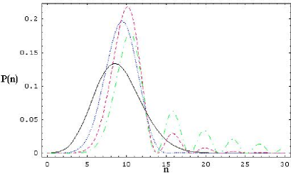
Figure 8: Photon number distribution for a squeezed state $|\alpha,r\rangle$, with $\alpha=3$ for several values of $r$: (a) $r=0$, i.e. coherent state (full line); (b) $r=0.5$ (dotted line); (c) $r=1$ (dashed line); (d) $r=1.5$ (dash-dotted line).

The mean photon number in the state $|\alpha,\varepsilon\rangle$ is made of two contributions: $\langle n\rangle=|\alpha|^{2}+|\nu|^{2}$, that is the sum of the average numbers of coherent and squeezed photons. The variance reads

$$\langle\Delta n^{2}\rangle=|\alpha\cosh r-\alpha^{*}e^{i\phi}\sinh r|^{2}+2\cosh^{2}r\sinh^{2}r\;.$$ (152)

By making use of the Hermitian phase operator $\Phi$ introduced by Pegg and Barnett [218], relation (152) allows to define number-phase squeezed states. These are states of minimum Heisenberg number-phase uncertainty $\langle\Delta n^{2}\rangle\langle\Delta\Phi^{2}\rangle=\frac{1}{4}$, just like coherent states [219], but one of the dispersions can get smaller than that of a coherent state. For particular choices of the phase $\theta$ of the complex field amplitude $\alpha=|\alpha|e^{i\theta}$ in Eq. (152), the corresponding state is called phase-squeezed state if the squeezing is $\pi/2$ out of phase with the complex field amplitude $(\phi=2\theta+\pi)$, or amplitude-squeezed state if the squeezing is in phase $(\phi=2\theta)$. The relation between quadrature and number squeezing is thoroughly explored in Ref. [40].

A further signature of nonclassicality of squeezed states is that, for them, the Glauber $P$-representation cannot be defined. However, other quasi-probability distribution functions exist for squeezed states, in particular the Husimi $Q$-function and the Wigner function. The latter, being the squeezed states Gaussian, is positive-defined.

The general quadratic Hamiltonian associated to the general Bogoliubov transformation, including a $c$-number term $\xi$: $b=\mu a+\nu a^{{\dagger}}+\xi$ takes the form [186]

$$H_{q}=f_{1}\left(a^{{\dagger}}a+\frac{1}{2}\right)+f_{2}^{*}a^{2}+f_{2}a^{{\dagger}2}+f_{3}^{*}a+f_{3}a^{{\dagger}}\;,$$ (153)

where $f_{i}$ are $c$-numbers, possibly time-dependent. The real coefficient $f_{1}$ is the free radiation energy of the mode $a$; the complex factor $f_{2}$ is the two-photon interaction energy; and, finally, $f_{3}$ is a linear forcing field (pump) associated to one-photon processes. The condition $f_{1}>2|f_{2}|$ assures that the Hamiltonian (153) is physical (positive-definite and bounded from below). It is moreover diagonalized to the form $H_{q}=\Omega(f_{1},f_{2})b^{{\dagger}}b+C(f_{1},f_{2},f_{3})$ by the transformation $b=\mu(f_{1},f_{2})a+\nu(f_{1},f_{2})a^{{\dagger}}+c(f_{1},f_{2},f_{3})$. A typical physical system associated to the quadratic form (153) is the degenerate parametric amplifier, which can be conveniently described by the Hamiltonian

$$H^{2ph}_{deg}=\omega a^{{\dagger}}a-[\eta^{*}e^{2i\omega t}a^{2}+\eta e^{-2i\omega t}a^{{\dagger}2}]\;.$$ (154)

The general solution of the Heisenberg equation of motion is then

$$a(t)=\cosh(|\eta|t)e^{-i\omega t}a+i\frac{\eta}{|\eta|}\sinh(|\eta|t)e^{-i\omega t}a^{{\dagger}}\;.$$ (155)

Exploiting relation (155), it can be easily shown that squeezed light generated from an initial vacuum state exhibits photon bunching, while for an initial coherent state the output light may be antibunched. This last effect marks a further characterization of the nonclassicality of squeezed states [220]. The methods introduced above can be generalized to define nondegenerate, multimode squeezed states. These states are obtained by successive applications on the vacuum state of the $n$-mode squeezing operator $S(\underline{\varepsilon})=e^{-\frac{1}{2}\varepsilon_{ij}a^{{\dagger}}_{i}a^{{\dagger}}_{j}+\frac{1}{2}\varepsilon_{ij}^{*}a_{i}a_{j}}$ and of the generalized displacement operator $D(\underline{\alpha})=e^{\alpha_{i}a^{{\dagger}}_{i}-\alpha_{i}^{*}a_{i}}$, where the Einstein summation convention on the repeated indices has been adopted, $\underline{\alpha}\equiv\{\alpha_{i}\}$, and $\underline{\varepsilon}\equiv\{\varepsilon_{ij}\}$ ($i,j=1,...,n$). We can then conveniently denote them as $|\underline{\alpha},\underline{\varepsilon}\rangle=D(\underline{\alpha})S(\underline{\varepsilon})|0\rangle$. We approach in some detail the important two-mode case, by considering two correlated modes $a_{1}$ and $a_{2}$ interacting according to bilinear Hamiltonians of the general form (145). A comprehensive framework for two-photon quantum optics was introduced by Caves and Schumaker in a beautiful series of papers [188]. They defined two-mode, linear canonical transformations as

$$b_{1}=\mu a_{1}+\nu a_{2}^{\dagger}\;,\quad\quad b_{2}=\mu a_{2}+\nu a_{1}^{\dagger}\;,$$ (156)

with the same parametrization of the complex coefficients as in the single-mode case. The transformed quasi-photon modes $(b_{1},b_{2})$ can also be obtained from the original mode variables by acting with the unitary operator

$$S_{12}(\zeta)=e^{{\zeta}^{*}a_{1}a_{2}-\zeta a_{1}^{\dagger}a_{2}^{\dagger}}\,,\quad\zeta=re^{i\phi}\;,$$

$$S_{12}\,a_{i}\,S_{12}^{{\dagger}}=a_{i}\cosh r+a_{j}^{{\dagger}}e^{i\phi}\sinh r\;,\quad i,j=1,2\;,i\neq j\;,$$ (157)

and two-mode squeezed states are defined as $|\alpha_{1},\alpha_{2};\zeta\rangle=D(\alpha_{1})D(\alpha_{2})S_{12}(\zeta)|0\rangle$. Equivalently, these states can be labelled by the complex eigenvalues of $b_{i}$: $b_{i}|\alpha_{1},\alpha_{2};\zeta\rangle=\beta_{i}|\alpha_{1},\alpha_{2};\zeta\rangle$ $(i=1,2)$, where $\beta_{i}=\alpha_{i}\cosh r+\alpha_{j}^{*}e^{i\phi}\sinh r$, $(i,j=1,2\;,\;i\neq j)$. The existence of nontrivial correlations between the modes is elucidated by computing the expectation values:

$$\langle a_{i}\rangle=\alpha_{i}\;,$$

$$\langle a_{i}^{{\dagger}}a_{j}\rangle=\alpha_{i}^{*}\alpha_{j}+\delta_{ij}\sinh^{2}r\;,$$

$$\langle a_{i}a_{j}\rangle=\alpha_{i}\alpha_{j}-(1-\delta_{ij})e^{i\phi}\sinh r\cosh r\;.$$ (158)

Among the interesting statistical properties of these states, an important role is played by the two-mode photon-number distribution, defined as the joint probability to find $n_{1}$ photons in the mode $a_{1}$ and $n_{2}$ photons in the mode $a_{2}$ [217]:

$$P(n_{1},n_{2})=|\langle n_{1},n_{2}|\alpha_{1},\alpha_{2};r\rangle|^{2}$$

$$=\left|\frac{(-\tanh r)^{p}}{\cosh r}\left(\frac{p!}{q!}\right)^{1/2}\mu_{1}^{n_{1}-p}\mu_{2}^{n_{2}-p}L_{p}^{(q-p)}\left(\frac{\mu_{1}\mu_{2}}{\tanh r}\right)e^{-\frac{1}{2}(\alpha_{1}^{*}\mu_{1}+\alpha_{2}^{*}\mu_{2})}\right|^{2},$$ (159)

where $\mu_{i}=\alpha_{i}+\alpha_{j}^{*}\tanh r$ with $(i,j=1,2\;,\;i\neq j)$, $p=min(n_{1},n_{2})$, $q=max(n_{1},n_{2})$ and $L_{l}^{(k)}(x)$ are generalized Laguerre polynomials. For a two-mode squeezed vacuum ($\alpha_{1}=\alpha_{2}=0$), the joint probability has only diagonal elements: $P(n,n)=(\tanh r)^{2n}/\cosh^{2}r$. More in general, for $\alpha_{1}=\alpha_{2}\neq 0$ the joint probability is obviously symmetric. In Figs. 9 (a)-(b) $P(n_{1},n_{2})$ is plotted at fixed squeezing $r=1.5$ and for two choices of the coherent amplitudes. Fig. 9 (a) shows asymmetric oscillations with the peaks being shifted due to the different coherent amplitudes. Fig. 9 (b) is instead characterized by the absence of oscillations.

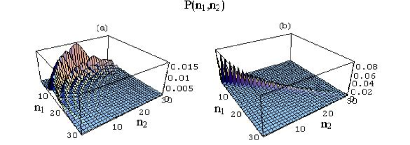
Figure 9: Photon number distributions for the two-mode squeezed state $|\alpha_{1},\alpha_{2};r\rangle$ with $r=1.5$ and (a) $\alpha_{1}=1$, $\alpha_{2}=3$, (b) $\alpha_{1}=-\alpha_{2}=2$.

Two-mode squeezed states are generated in the dynamical evolution of a nondegenerate parametric amplifier, described by the total Hamiltonian

$$H^{2ph}_{T}=H^{2ph}_{0}+H^{2ph}_{I}=\omega_{1}a_{1}^{{\dagger}}a_{1}+\omega_{2}a_{2}^{{\dagger}}a_{2}+i\chi(a_{1}^{{\dagger}}a_{2}^{{\dagger}}e^{-2i\omega t}-a_{1}a_{2}e^{2i\omega t})\;,$$ (160)

where the coupling constant $\chi$ is assumed real without loss of generality. The solutions of the Heisenberg equations of motion in the interaction picture are

$$a_{1}(t)=a_{1}\cosh\chi t+a_{2}^{{\dagger}}\sinh\chi t\;,\quad a_{2}(t)=a_{2}\cosh\chi t+a_{1}^{{\dagger}}\sinh\chi t\;,$$ (161)

so that, as expected, the conservation law $n_{1}(t)-n_{2}(t)=n_{1}(0)-n_{2}(0)$ holds. Choosing an initial two-mode coherent state $|\alpha_{1}\rangle|\alpha_{2}\rangle$, the mean photon number in each mode evolves as

$$\langle n_{i}(t)\rangle\,=\,|\alpha_{i}\cosh\chi t+\alpha_{j}^{*}\sinh\chi t|^{2}\,+\,\sinh^{2}\chi t\;,\quad i,j=1,2\;,i\neq j\;,$$ (162)

with the last term representing the amplification of vacuum fluctuations. A further, important signature of nonclassicality stems from the fact that, if the system is initially in the vacuum state, the intensity cross-correlation, defined by $\langle n_{1}(t)n_{2}(t)\rangle$, maximally violates the classical Cauchy-Schwartz inequality $(\langle n_{1}n_{2}\rangle)^{2}\leq\langle a^{{\dagger}2}_{1}a_{1}^{2}\rangle\langle a^{{\dagger}2}_{2}a_{2}^{2}\rangle$ [22].

4.4 An interesting case of four-wave mixing: degenerate three-photon down conversion

The degenerate three-photon down conversion $3\omega\rightarrow\omega+\omega+\omega$ is the next natural step to be considered beyond the two-photon down conversion processes. The interaction Hamiltonian of degenerate three-photon down conversion reads

$$H_{I}^{3dc}=\kappa a^{{\dagger}3}b+\kappa^{*}a^{3}b^{{\dagger}}\;,$$ (163)

where the modes $a$ and $b$ are the down-converted signal and the quantized pump, respectively. The interaction can be realized in a $\chi^{(3)}$ medium and the Hamiltonian (163) can be derived by Eq. (89). The process has been studied theoretically for running waves (OPA) [221, 222, 223, 224, 225, 226, 227, 228] and for optical cavities (OPO) [229], and in general the time evolution generated by Hamiltonian (163) cannot be expressed in closed, analytical form. Analogously to the two-photon case, a physical simplification is obtained by applying the parametric approximation to the pump mode (considered coherent and intense) $b\rightarrow\beta$ ($\beta$ $c$-number). In this approximation $H_{I}^{3dc}$ reduces to

$$H_{I}^{3dcp}\,=\,\xi a^{{\dagger}3}\,+\,\xi^{*}a^{3}\;,$$ (164)

where the time-independent complex parameter $\xi$ is proportional to the pump amplitude $\beta$. Since in both cases disentangling formulas for the evolution operators do not exist, it is then necessary to resort to numerical methods in order to study the dynamics of the process. Moreover, the evolution operator for the Hamiltonian (164) suffers of divergences [221], that need to be treated by specific summation techniques [222]. In Ref. [224] Elyutin and Klyshko showed that the average output energy $\langle n\rangle$ of the parametric amplifier $H_{I}^{3dcp}$ diverges infinity after a finite time lapse $t_{0}$. The dynamics for $n$ can be cast in the form:

$$\ddot{n}\,=\,6n^{2}+6n+4\;,$$ (165)

and, after some manipulations, an exact expression for the average value $N(\tau)\equiv\langle n\rangle(\tau)$ (with $\tau=\kappa t$ rescaled, dimensionless time) can be expressed in the form of a Taylor series. As an example, if we choose the vacuum as the initial state, then

$$N(\tau)=2\tau^{2}+4\tau^{4}+11.2\tau^{6}+34.8\tau^{8}+...\;.$$ (166)

We see that the explosion time $\tau_{0}$ is clearly finite; it can be defined as the convergence radius of the series (166) obtained by an extrapolation of the coefficients in Eq. (166) that yields $\tau_{0}\simeq 0.53$ [224]. This is at striking variance with the case of two-photon down conversion, where such a divergence occurs only in the limit of infinite time. The existence of a finite explosion time shows a pathology of the perturbative techniques, that consequently need to be treated with some care. This and related problems will be discussed further in the next Section, but here we first move on to illustrate some interesting properties of the Wigner function for the states generated by the fully quantized Hamiltonian (163). Concerning OPO dynamics, Felbinger et al. [229] studied, using quantum trajectory simulations, three-photon down conversion in an optical cavity resonant at the frequencies $\omega$ and $3\omega$. The authors included homodyne detection and quantum state reconstruction setups, and considered, besides the three-photon down conversion interactions, the simultaneous presence of Kerr and cross-Kerr terms of the type $a^{{\dagger}2}a^{2}\;,b^{{\dagger}2}b^{2}\;,a^{{\dagger}}ab^{{\dagger}}b$. They were able to determine the Wigner function for the intracavity and extracavity fields, and, in the case of the intracavity mode, showed that it is non Gaussian, non-negative, and exhibits a threefold symmetry with respect to three directions in phase space (“star states”). Concerning OPA dynamics, Banaszek and Knight [228] studied the evolution of the signal mode under the action of the Hamiltonian (163) for the initial state $|0\rangle_{a}|\beta\rangle_{b}$ and calculated numerically the Wigner function for the reduced density operator $\rho_{b}(t)=Tr_{b}[e^{-itH_{I}^{3dc}}|0\rangle_{a}|\beta\rangle_{b}\,{}_{b}\langle\beta|_{a}\langle 0|e^{itH_{I}^{3dc}}]$. The Wigner function exhibits a deep nonclassical behavior, again possessing three arms with a star-symmetry in phase space, and a typical interference pattern in the regions delimited by the three arms. The authors developed a very interesting approximate analytical description of such a pattern (based on a coherent superposition of distinct phase-space components), that here we briefly summarize. Let us assume that the wave function $\psi(x)$ can be approximately written as superposition of a finite number of components:

$$\psi(x)\simeq\sum_{i}\mathcal{A}_{i}(x)e^{i\Phi_{i}(x)}\;,$$ (167)

where $\mathcal{A}_{i}(x)$ are slowly varying positive envelopes and $\Phi_{i}(x)$ are real functions defining the phases. The corresponding Wigner function reads

$$W(x,p)=$$

$$\frac{1}{2\pi}\sum_{i,j}\int dy\mathcal{A}_{i}\left(x-\frac{y}{2}\right)\mathcal{A}_{j}\left(x+\frac{y}{2}\right)e^{-ipy-i\Phi_{i}\left(x-\frac{y}{2}\right)+i\Phi_{j}\left(x+\frac{y}{2}\right)}\;.$$ (168)

Assuming the stationary-phase approximation $\Phi^{\prime}_{i}\left(x-\frac{y}{2}\right)+\Phi^{\prime}_{j}\left(x+\frac{y}{2}\right)=2p$ (where the prime denotes the first derivative), the contribution to the Wigner function at the point $(x,p)$ comes from the points of the trajectories $[x_{i};p_{i}=\Phi^{\prime}_{i}(x)]$ and $[x_{j};p_{j}=\Phi^{\prime}_{j}(x)]$, satisfying the relations $x_{i}+x_{j}=2x$ and $p_{i}+p_{j}=2p$. By fixing a pair of values $(x,p)$, the corresponding pair $x_{i},x_{j}$ is determined by the two previous constraints and by the expression of the phases. Taking the value of the envelope at the point $x_{i}$, expanding the phases up to quadratic terms, and performing the associated Gaussian integrals, the approximate form of the Wigner function is

$$W(x,p) \approx\sum_{i}\mathcal{A}_{i}^{2}(x)\delta(p-\Phi^{\prime}_{i}(x))$$ (169)

$$+\sum_{i\neq j}\sum_{x_{i},x_{j}}\frac{\sqrt{2}\mathcal{A}_{i}(x_{i})\mathcal{A}_{j}(x_{j})}{\sqrt{\pi i[\Phi^{\prime\prime}_{i}(x_{i})-\Phi^{\prime\prime}_{j}(x_{j})]}}e^{ip(x_{i}-x_{j})-i\Phi_{i}(x_{i})+i\Phi_{j}(x_{j})}\;.$$

Specializing to the case of three-photon down conversion processes, it can be shown that the arms of the Wigner function can be modelled by the three components of the wave function $\psi(x)$

$$\psi(x) = \sum_{i=1}^{3}\psi_{\theta_{i}}(x)$$ (170)

$$= \mathcal{A}(x)+\sqrt{2}\mathcal{A}(-2x)e^{\frac{\sqrt{3}}{2}ix^{2}-i\frac{\pi}{6}}+\sqrt{2}\mathcal{A}(-2x)e^{-\frac{\sqrt{3}}{2}ix^{2}+i\frac{\pi}{6}}\;,$$

where, as we will see soon, the angles $\theta_{i}$ are connected to rotations in phase space. The three components $\psi_{\theta_{i}}$ are obtained in the following way. By considering a slowly varying positive function $\mathcal{A}(x)$ one defines $\psi_{\theta_{1}}(x)\equiv\psi_{0}(x)=\mathcal{A}(x)$. Then one obtains the other components performing rotations around the origin of the phase space: $U(\theta)=e^{-i\theta a^{{\dagger}}a}$. Using the configuration representation of the rotation operator, and choosing in a suitable way the rotation angles $\theta_{2}$ and $\theta_{3}$, the other two components in Eq. (170) are obtained. Applying Eq. (169), the Wigner function is approximated by the expression

$$W_{\psi}(x,p)\,=\,W_{\psi_{\theta_{1}}}(x,p)+W_{\psi_{\theta_{2}}}(x,p)+W_{\psi_{\theta_{3}}}(x,p)+W_{int}(x,p)\;,$$ (171)

where $W_{int}(x,p)$ is the interference term responsible for the nonclassical nature of the state: due to $W_{int}(x,p)$, plotted in Fig. (10), the total Wigner function exhibits strong interference patterns and oscillations, and becomes negative in several regions of phase space.

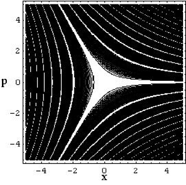
Figure 10: Contour plot of the interference pattern $W_{int}(x,p)$.

Banaszek and Knight have shown that there is excellent agreement between the Wigner function computed by exact numerical methods and the one obtained by the approximate analytical method that we have just described. This fact suggests that such a technique might be suitable for application to other instances of (degenerate) multiphoton processes.

4.5 Kerr nonlinearities as a particularly interesting case of four-wave mixing. A first discussion on the engineering of nonclassical states and macroscopic quantum superpositions

A particular and important subclass of third-order multiphoton processes described by the four-wave mixing Hamiltonian (133) is selected in the cases of total degeneracy, yielding the Kerr interaction $a^{{\dagger}2}a^{2}$ (self-phase modulation effect), and in the partially degenerate case, yielding the cross-Kerr interaction $a^{{\dagger}}b^{{\dagger}}ab$ (cross-phase modulation effect). In the presence of two optical frequencies, $\omega_{s}$ (signal) and $\omega_{p}$ (probe), and by using the expression (79) for the electric field operator, the interacting part of Hamiltonian (77) with $n=3$ reads

$$H_{Kerr} = \lambda_{s}[\chi^{(3)}(\omega_{s};\omega_{s},-\omega_{s},\omega_{s})a^{{\dagger}}_{s}a_{s}a^{{\dagger}}_{s}a_{s}\,+\,5\mathcal{F}(a^{{\dagger}}_{s},a_{s})]$$ (172)

$$+ \lambda_{p}[\chi^{(3)}(\omega_{p};\omega_{p},-\omega_{p},\omega_{p})a^{{\dagger}}_{p}a_{p}a^{{\dagger}}_{p}a_{p}\,+\,5\mathcal{F}(a^{{\dagger}}_{p},a_{p})]$$

$$+ \lambda_{sp}[\chi^{(3)}(\omega_{p};\omega_{p},-\omega_{s},\omega_{s})a^{{\dagger}}_{p}a_{p}a^{{\dagger}}_{s}a_{s}+23\mathcal{F}(a^{{\dagger}}_{p},a_{p},a^{{\dagger}}_{s},a_{s})]\;,$$

where $\lambda_{s}$, $\lambda_{p}$, and $\lambda_{sp}$ are real constants, $\mathcal{F}$ contains terms in which the order of the arguments is interchanged with respect to the Kerr terms written down explicitely, and the associated nonlinear processes are automatically phase matched. The final form of the normal ordered Hamiltonian is

$$H_{Kerr}\,=\,\chi_{s}a^{{\dagger}2}_{s}a^{2}_{s}\,+\,\chi_{p}a^{{\dagger}2}_{p}a^{2}_{p}\,+\,\chi_{sp}a^{{\dagger}}_{s}a^{{\dagger}}_{p}a_{s}a_{p}\;,$$ (173)

where the nonlinear couplings $\chi_{s}$, $\chi_{p}$, and $\chi_{sp}$ are simple combinations of the original couplings. It is worth noting that Kerr interactions are important in quantum optics because of their crucial role in the realization of nonlinear devices, such as quantum nondemolition meters, nonlinear couplers, and interferometers. Moreover, they are important in quantum state engineering, e.g. in the realization of macroscopic superpositions and entangled states. In some applications, as quantum nondemolition measurements of the photon number, it could be necessary to remove one or both of the self-phase modulation effects. This task can be accomplished by resorting to different strategies; for example, the cross-Kerr process can be favored by resonance conditions under which the other terms become negligible. Another possibility consists in the cancellation of the undesired self-phase modulation term by means of an auxiliary medium with negative $\chi^{(3)}$ (two-crystal configuration), in the sense that the undesired term is cancelled out if the corresponding field passes through another negative $\chi^{(3)}$ medium.
Here we begin by discussing the possibility of using a Kerr medium to perform quantum nondemolition (QND) measurements. The latter are important for many applications in modern quantum physics, and essentially consist in measuring an observable with exact precision at the expense of an increasing uncertainty of its canonically conjugated observable. An excellent discussion of QND measurements can be found in the review by Braginsky and Khalili [230]. Here we illustrate the Kerr-based scheme proposed by Imoto, Haus, and Yamamoto [231, 232] and depicted in Fig. (11). It represents a nonlinear interferometer, that is a Mach-Zehnder interferometer with a Kerr medium placed in one of the arms [189, 233, 234].

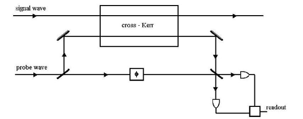
Figure 11: Experimental setup (Mach-Zehnder interferometric detector) for a quantum nondemolition measurement of the photon number through the cross-Kerr effect.

A signal and a probe wave, respectively at frequencies $\omega_{s}$ and $\omega_{p}$, propagate in the optical Kerr medium. Because of the cross-Kerr effect $\chi_{sp}n_{s}n_{p}$ ($n_{s}=a^{{\dagger}}_{s}a_{s}\;,\;n_{p}=a^{{\dagger}}_{p}a_{p}$), the photon number $n_{s}$ modulates the phase of the probe wave, and a measurement of this modulation yields the information about the $n_{s}$ itself. Let $a_{s}^{in}$ and $a_{p}^{in}$ denote the input operators for the signal and the probe waves; the corresponding output operators can be determined explicitly, by solving the Heisenberg equations, and read:

$$a_{s}^{out}(\tau)\,=\,e^{i\tau n_{p}}a_{s}^{in}\;,\quad a_{p}^{out}(\tau)\,=\,e^{i\tau n_{s}}a_{p}^{in}\;,$$ (174)

with the dimensionless time $\tau=\chi_{sp}t$. Moreover, a phase difference $\phi=\pi/2$ is imposed between the two arms of the detector, and the two photodiode currents are subtracted as shown in the scheme Fig. (11). Introducing the quadrature operators $X_{i}^{l}\equiv(a_{i}^{l}+a_{i}^{{\dagger}\,l})/\sqrt{2}$ and $P_{i}^{l}\equiv i(a_{i}^{{\dagger}\,l}-a_{i}^{l})/\sqrt{2}$, with $i=s,p$ and $l=in\,,out$, the readout observable corresponding to the difference current is the output probe quadrature phase amplitude

$$P_{p}^{out}\,=\,X_{p}^{in}\sin(\tau n_{s})\,+\,P_{p}^{in}\cos(\tau n_{s})\;.$$ (175)

Fixing the input probe phase such that $\langle P_{p}^{in}\rangle=0$, relation (175) can be approximated (for small $\chi_{sp}$) as

$$P_{p}^{out}\simeq\langle X_{p}^{in}\rangle\tau n_{s}+\Delta P_{p}^{in}\;,$$ (176)

where $\Delta P_{p}^{in}=P_{p}^{in}-\langle P_{p}^{in}\rangle\equiv P_{p}^{in}$. A normalized readout observable $n_{s}^{(obs)}$ corresponding to the signal photon number can be defined as

$$n_{s}^{(obs)}\equiv\frac{P_{p}^{out}}{\langle X_{p}^{in}\rangle\tau}=n_{s}+\frac{\Delta P_{p}^{in}}{\langle X_{p}^{in}\rangle\tau}\,.$$ (177)

Thus the measured observable is $\langle n_{s}^{(obs)}\rangle=\langle n_{s}\rangle$, and its variance is given by

$$\langle(\Delta n_{s}^{(obs)})^{2}\rangle=\langle\Delta n_{s}^{2}\rangle+\frac{\langle(\Delta P_{p}^{in})^{2}\rangle}{\langle n_{p}\rangle\tau^{2}}\;,$$ (178)

which holds, for instance, if the probe wave is in a coherent state, with $\langle(\Delta P_{p}^{in})^{2}\rangle=1/4$. Therefore, for increasing $\langle n_{p}\rangle\tau^{2}$, the measured uncertainty tends to the ideal value $\langle\Delta n_{s}^{2}\rangle$, that is the intrinsic uncertainty of the observable $n_{s}$. At the same time, as a result of the measurement, an increase of the quantum uncertainty of the probe wave photon number is obtained. The scheme exposed above well represents the main features of a quantum nondemolition measurement. Of course, many other proposals have been used based on the extension or modification of this scheme, and for different purposes [236, 237, 238, 239, 240]. Kitagawa, Imoto, and Yamamoto have exploited the quantum nondemolition measurement via the cross-Kerr effect to produce number-phase minimum uncertainty states and near-number states [236]. Losses have been taken into account as well, for example in Ref. [237], the scheme has been extended to optical cavities [238, 239], and the effect of quantum nondemolition measurements on quantum interference has been also investigated [240]. Finally, photon-number measurements have been realized in optical fibers [241, 242], and by exploiting atoms in a cavity [243, 244].

Many other Kerr-based nonlinear devices, beyond the interferometric setup described in Fig. (11), have been proposed in the literature; here we limit ourselves to the discussion of two significant examples. The nonlinear directional coupler [245, 246] consists of two parallel waveguides, exhibiting third-order nonlinearity, that exchange energy by means of evanescent waves. The general Hamiltonian reads

$$H_{coup}\,=\,H_{Kerr}\,+\,\lambda a_{s}a^{{\dagger}}_{p}\,+\,\lambda^{*}a^{{\dagger}}_{s}a_{p}\;,$$ (179)

where $H_{Kerr}$ is given by Eq. (173), and the last two terms are the evanescent-waves contribution. This system presents interesting properties such as self-trapping, self-modulation, and self-switching of the energy of the coupled modes [247], and it can be useful for the generation and transmission of nonclassical light. The Kerr couplers can produce sub-Poissonian squeezed light [248, 249, 250], and entangled states [251]. We want also to mention another interesting device, named nonlinear quantum scissor, that has been proposed to perform optical state truncation [252, 253]. It can be realized by means of a fully degenerate Kerr medium in an optical cavity, pumped by external ultra-short pulses of laser light [253]. The optical state truncation that can be achieved allows, under suitable conditions [253], the reduction of an initial coherent state even up to a single-photon Fock state. It is worth noting that such a device can be realized by means of linear optical components and photo-detections as well [254].

Concerning Kerr-based quantum state engineering, nonlinear interferometric devices have been largely considered for the generation of nonclassical states of the radiation field [255, 256, 257, 258, 259], such as, specifically, the entangled coherent states of the form $(e^{-i\pi/4}|i\beta\rangle_{1}|i\alpha\rangle_{2}+e^{i\pi/4}|-\alpha\rangle_{1}|\beta\rangle_{2})/\sqrt{2}$ discussed in Ref. [255]. Nonlinear Mach-Zehnder-type interferometers have been proposed for the production of maximally entangled number states of the form

$$|\Psi\rangle_{MES}\,=\,\frac{1}{\sqrt{2}}(|N\rangle_{a}|0\rangle_{b}\,+\,e^{i\Phi_{N}}|0\rangle_{a}|N\rangle_{b})\;.$$ (180)

A first proposal to produce them [257] is based on a setup employing the Fredkin gate [260] (based on a cross-Kerr interaction) in a double-interferometer configuration. Another proposal [258] relies on the use of a four-wave mixer, described by the interaction Hamiltonian $H_{int}=\chi^{(3)}(a^{{\dagger}}b+ab^{{\dagger}})^{2}$, in one arm of the interferometer, that contains both cross-Kerr and nonlinear birefringence terms. States (180) are potentially important for applications in metrology, as atomic frequency measurements [261], and interferometry [262]. Moreover, these states show phase super-sensitivity, in the sense that they reduce the phase uncertainty to the Heisenberg limit $\Delta\phi_{HL}=1/N$. These states have not yet been produced in nonlinear devices; however, in recent successful experiments, their three-photon ($N=3$) [263] and four-photon ($N=4$) [264] versions have been realized by means of linear optical elements and photodetections.

The engineering of quantum states by use of Kerr media includes the generation of optical “macroscopic” superpositions of coherent states. Macroscopic (or mesoscopic) superpositions take the form $|\psi\rangle=c_{1}|\alpha e^{i\theta}\rangle+c_{2}|\alpha e^{-i\theta}\rangle$, where $|\alpha e^{\pm i\theta}\rangle$ are coherent states with a sufficiently high average number of photons $|\alpha|^{2}$. In the course of the years, many proposals have been put forward for the generation of such ”Schrödinger cat” superpositions. Among them, we should mention schemes based on state reduction methods [265], and on conditional measurements performed on entangled states [266]. However, the simplest way (at least from a theoretical point of view) to obtain macroscopic superpostions is the propagation of the radiation field through an optical fiber associated with nonlinear Kerr effects and interactions [234, 267, 268, 269, 270, 271]. Schrödinger cat states possess important nonclassical properties [272, 273] like squeezing and sub-Poissonian statistics, moreover they should provide the crucial playground for the testing of the quantum-classical transition and the theory of decoherence.
In 1986, generalizing the model studied by Milburn and Holmes [267], Yurke and Stoler [268] considered the time evolution of an initial coherent state under the influence of the anharmonic-oscillator Hamiltonian:

$$H_{anh}\,=\,\omega n\,+\,\Omega n^{k}\;,\quad(k\geq 2)\;,$$ (181)

where $\omega$ is the energy-level splitting for the harmonic-oscillator part of the Hamiltonian, $\Omega$ is the strength of the anharmonic term, and $n$ is the number operator. In a nonlinear medium $\Omega$ is proportional to the $(k+1)$-th order nonlinearity. Note that, for $k=2$, the anharmonic part of the Hamiltonian is of the degenerate, single-mode Kerr form, apart an additive term linear in $n$ that simply amounts to an irrelevant constant rotation in phase space. Yurke and Stoler evaluated the response of a homodyne detector to the evolved state

$$|\alpha,t\rangle\,=\,e^{-it\Omega n^{k}}|\alpha\rangle\,=\,e^{-\frac{|\alpha|^{2}}{2}}\sum_{n=0}^{\infty}\frac{\alpha^{n}e^{-i\phi_{n}(t)}}{\sqrt{n!}}|n\rangle\;,$$ (182)

where $\phi_{n}(t)=\Omega tn^{k}$. The state vector is periodic with period $2\pi/\Omega$, and coherent superpositions of distinguishable states of the radiation field emerge for special values of $t$; for instance:

$$|\alpha,\pi/2\Omega\rangle = \frac{1}{\sqrt{2}}[e^{-i\pi/4}|\alpha\rangle+e^{i\pi/4}|-\alpha\rangle]\;,\quad k\;\;even\;,$$ (183)

$$|\alpha,\pi/2\Omega\rangle = \frac{1}{2}[|\alpha\rangle-|i\alpha\rangle+|-\alpha\rangle+|-i\alpha\rangle]\;,\quad k\;\;odd\;.$$ (184)

A very useful insight on the properties of states (183) and (184) is gained by looking at their Wigner functions, which are plotted, respectively for even and odd $k$ in Fig. (12)-(a) and (12)-(b). They show a typical two- and four-lobe structure, representing the coherent state components, and evident fringes due to quantum interference.

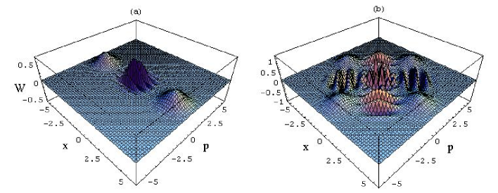
Figure 12: Figure (a): Wigner function for the even Schrödinger cat states Eq. (183). Figure (b): Wigner function for the odd Schrödinger cat states Eq. (184). In both cases, the coherent amplitude $\alpha=3$.

The coherence properties are very sensitive to losses as shown, using coherent superpositions of the form (183), in Ref. [268] by Yurke and Stoler: for macroscopic coherent inputs, corresponding to large mean photon numbers $|\alpha|^{2}$, even a very small amount of loss, corresponding to nonideal detection efficiency, destroys the interference fringes and leads to a probability distribution for the homodyne-detector’s output current indistinguishable from that of a classical statistical mixture of coherent states, see Fig. (13) (a).
In Ref. [269] Mecozzi and Tombesi have suggested to extend the method of Yurke and Stoler by considering more general Kerr-like Hamiltonians $H_{gK}$ of the form $H_{gK}=H_{0}+\lambda(H_{0})^{2}$, with $H_{0}$ any diagonalizable Hamiltonian. Although the original aim of the authors was to discuss the decoherence effects due to vacuum fuctuations, as we will see in the following, we can take a special realization of their general Hamiltonian $H_{gK}$ in order to compare directly with the original scheme of Yurke and Stoler and highlight the role of squeezing (and in general of nonclassicality) in improving the preservation of coherence against losses. To this aim, let us in fact choose the particular $H_{0}=b^{{\dagger}}b$, with $b$ denoting the canonically transformed Bogoliubov quasi-photon mode: $b=\mu a+\nu a^{{\dagger}}$. With this choice, following the line of thought of Yurke and Stoler, we consider the evolution generated by the Hamiltonian $H_{gK}$ applied to an initial squeezed state (the eigenstate of mode $b$). Comparing Figures (13) (a) and (b) shows that, for the same amount of losses that destroy the coherence in the Yurke-Stoler scheme, a finite amount of squeezing is more effective in fighting decoherence, as witnessed by the persistent visibility of the interference fringes.

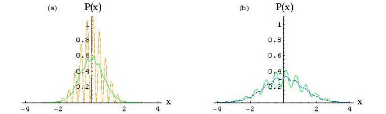
Figure 13: In these figures we compare the behavior of the interference fringes associated to the cat states of Yurke and Stoler (Fig. (a)), and those associated to the superposition states generated through the modified quasi-particle Kerr Hamiltonian $H_{gK}$ (Fig. (b)). In both cases, the superposition states are sent in one input port of a beam splitter of transmittance $\eta$, while the other input port is taken empty. The beam splitter can be used to model medium or detector losses, which are quantified by the transmittance $\eta$. The $x$-axes corresponds to the homodyne variable measured at the first output port of the beam splitter. The $y$-axes corresponds to the probability distributions $P(x)$ for the homodyne variable $x$ detected at the first output port independently of what has left the second output port. In Figure (a) the dotted line represents the interference fringes obtained with the Yurke-Stoler scheme in the case of perfect transmittance $\eta=1$, and the full line represents the fringes in the same scheme with transmittance $\eta=0.96$. In Figure (b), the full line represents the fringes associated to the scheme based on the modified quasi-particle Kerr Hamiltonian $H_{gK}$ for $\eta=0.96$, and the dashed line represents the fringes obtained in the same scheme for $\eta=0.9$. In either case the squeezing parameter is fixed at the value $r=0.4$. The mean number of photons in the initial states, in all cases here considered, is equal to $36$. From Figure (a), we see that the interference fringes, which are evident in the ideal $\eta=1$ case, practically disappear even for a slight amount of loss in the transmittance. Figure (b) shows that the action of the squeezing, although lowering the primary peak of the fringes, moves down the threshold of complete decoherence from $\eta=0.96$ to $\eta=0.9$.

For a degenerate Kerr Hamiltonian $\Omega\;a^{{\dagger}2}a^{2}$, a more general class of superposition states is generated at times $t=\pi/m\Omega$ with $m$ an arbitrary, nonzero integer [274]:

$$|\psi(t=\pi/m\Omega)\rangle=e^{-\frac{i\pi}{m}n(n-1)}|\alpha\rangle$$ (187)

$$=\left\{\begin{array}[]{rrr}\sum_{q=0}^{m-1}f_{q}^{(e)}|\alpha e^{-\frac{2\pi iq}{m}}e^{i\frac{\pi}{m}}\rangle\;,&f_{q}^{(e)}=\frac{1}{m}\sum_{n=0}^{m-1}e^{\frac{2\pi iq}{m}n}e^{-\frac{i\pi}{m}n^{2}}\;,&\quad m\;even\;,\\ &&\\ \sum_{q=0}^{m-1}f_{q}^{(o)}|\alpha e^{-\frac{2\pi iq}{m}}\rangle\;,&f_{q}^{(o)}=\frac{1}{m}\sum_{n=0}^{m-1}e^{\frac{2\pi iq}{m}n}e^{-\frac{i\pi}{m}n(n-1)}\;,&\quad m\;odd\;.\end{array}\right.$$

(188)

Interestingly, these superpositions of arbitrary finite length are eigenstates of $a^{m}$, and thus have a suggestive interpretation in terms of “higher-order” coherent states. In fact, the nonlinear refractive index of the Kerr medium acts on the input field by modifying the phase-sensitive quantum noise. For an input coherent state this leads to ”self-squeezed” light [275], in the sense that the initial coherent state acts itself as a “self-pump”, playing the role of a linear driving field. However, the Kerr effect does not change the photon statistics, which, if the input is coherent, remains Poissonian.
The production of two-mode (entangled) optical Schrödinger cats via the two-mode Kerr interaction (173) has been investigated as well [276]. To insure the time-periodicity of the state vectors, the parameters $\Delta=\omega_{s}-\omega_{p}$, $\chi_{s}$, $\chi_{p}$, and $\chi_{sp}$ must be chosen mutually commensurate. In the resonant case $\Delta=0$, with the choices $\chi_{s}=\chi_{p}$, $\chi_{sp}/\chi_{p}=1.2$, and initial two-mode coherent state $|\alpha,\beta\rangle$, the following coherent superposition is generated at the reduced, adimensional time $\tau\doteq\chi_{s}t=5\pi/2$:

$$|\alpha,\beta,\,\tau=5\pi/2\rangle\,=\,\frac{1}{\sqrt{2}}\{e^{-i\pi/4}|i\alpha,i\beta\rangle\,+\,e^{i\pi/4}|-i\alpha,-i\beta\rangle\}\;.$$ (189)

Macroscopically distinguishable quantum states can also be produced exploiting nonlinear birefringence, as shown by Mecozzi and Tombesi [269] and by Yurke and Stoler [270]. Mecozzi and Tombesi considered the effective Hamiltonian

$$H\,=\,\omega(a^{{\dagger}}a+b^{{\dagger}}b)\,+\,\kappa(ab^{{\dagger}}-a^{{\dagger}}b)\,+\,\frac{\Omega}{2}(ab^{{\dagger}}+a^{{\dagger}}b)^{2}\;,$$ (190)

where the modes $a$ and $b$ represent the two orthogonal polarizations of a coherent light beam entering the birefringent medium. Moreover, Mecozzi and Tombesi showed that the vacuum fluctuations can be suitably removed by injecting in the unused port a squeezed vacuum.
A similar Hamiltonian was considered by Agarwal and Puri to study the one-dimensional propagation of elliptically polarized light in a Kerr medium [277]. The study of this kind of processes leads to an interesting result, essentially due to the quantum nature of the field; it consists in the possibility that the degree of polarization may change with time, leading, for some times, to a partially polarized field, in contrast to the one coming from semiclassical theory which predicts a constant polarization.
For completeness, we point out that multicomponent entangled Schrödinger cat states can be in principle generated by the dynamics associated to a fully quantized nondegenerate four-wave mixing process, described by the effective interaction Hamiltonian $H_{ndg}^{4wm}=\kappa(a^{{\dagger}}b+b^{{\dagger}}a)(c^{{\dagger}}d+d^{{\dagger}}c)$, with $a$ and $c$ taken as the pump modes, and $b$ and $d$ taken as the signal modes [278].

Regarding the possibility of experimental realizations of macroscopic superpositions in a Kerr medium, the quite small values of the available Kerr nonlinearities would require, for the generation of a cat state, a long interaction time, or equivalently a large interaction length. For an optical frequency of $\omega\approx 5\times 10^{14}\;rad\;sec^{-1}$, one would need an optical fiber of about $1500$ km, and, consequently, losses and decoherence would destroy completely the quantum superpositions. However, in recent years there have been some interesting theoretical proposals aimed at overcoming these difficulties and obtaining cat states in the presence of small Kerr effects. One of the most recent and feasible proposals [279] is based on the following scheme: a Kerr-evolved state (188) and the vacuum feed the two input ports of a $50-50$ beam splitter; after passing the beam splitter, the real part of the coherent amplitude of the resulting two-mode output state is measured by homodyne detection, reducing to a new finite superposition of coherent states. Suitably engineering the coefficients of this superposition leads to a Schrödinger cat. This scheme allows to produce cat states of high quality without requiring a strong nonlinearity. In fact, in this scheme, based on the successive application of Kerr interaction, beam splitter, and, finally, homodyne detection, the time needed to produce the Schrödinger cat state practically coincides with the time needed to produce the Kerr-evolved state of the form (188). Therefore, choosing for instance in Eq. (188) $m\simeq 10^{2}$, the equivalent length of the optical fiber needed to produce the cat is reduced to few tens of kilometers, and this in turn greatly reduces the effect of losses and dispersion. Further improvements along this line may be thus expected in the near future. However, as we will see in the next Section, methods based on high-$Q$ cavity fields have proved more effective than fibers in the experimental production of mesoscopic coherent superpositions.

4.6 Simultaneous and cascaded multiphoton processes by combined three- and four-wave mixing

Most of the interaction Hamiltonians used in multiphoton quantum optics deal with a single parametric process, but in the two last Subsections we have already met some examples of coexisting, concurring interactions. At present the possibility to produce quantum states with enhanced nonclassical properties, the need to take into account more than one nonlinear contribution, and the complexity in experimental engineering, have promoted the idea to exploit composite, concurrent multiphoton interactions. These can be realized in several ways through multi-step, cascaded schemes either in the same nonlinear medium, or by using different media in a suitable experimental configuration. In this Subsection we describe some models and schemes based on multiphoton multiple processes and interactions.
Let us first consider some examples of combinations of two different nonlinear processes occurring inside the same crystal. A simple multiphoton interaction Hamiltonian involving two different nonlinear terms was studied by Tombesi and Yuen [280] in order to improve the maximum available squeezing of the standard optical parametric amplifier (OPA). They considered the short-time interaction of a single-mode coherent light with an optically bistable two-photon medium that combines Kerr-type effects and degenerate down conversion, and gives rise to the interaction Hamiltonian

$$H_{I}^{SK}\,=\,i\kappa(a^{2}-a^{{\dagger}2})\,+\,\Omega a^{{\dagger}2}a^{2}\;,$$ (191)

with $\kappa$ and $\Omega$ real. Later, the time evolution of the Hamiltonian (191) was studied by Gerry and Rodrigues [281] for longer times by means of a numerical method. Assuming a coherent state as the initial input state, Gerry and Rodrigues verified the presence of squeezing and antibunching effects recurring on a longer time scale. Hamiltonian models of the form (191) have also been studied in cavity, both for the one-mode [282] and the two-mode case [283].
Concurrent, two-step optical $\chi^{(2)}$-interactions were observed for the first time in 1970, using ammonium dihydrogen phosphate as a medium [284]. In this experiment the crystal was illuminated by a classical laser pump at frequency $\omega_{p}$ with equal ordinary and extraordinary polarization components $\omega_{p}^{o}\equiv\omega_{p}^{e}$; the simultaneous collinear phase matching was obtained for the spontaneous down conversion process $\omega_{p}^{e}\rightarrow\omega_{i}^{o}+\omega_{1}^{e}$, and the successive up conversion process $\omega_{p}^{o}+\omega_{i}^{o}\rightarrow\omega_{2}^{e}$ where $\omega_{i}^{o}$, $\omega_{1}^{e}$, $\omega_{2}^{e}$ represent, respectively, the one idler, and the two signal modes. Few years later, the quantum theory of coupled parametric down-conversion and up-conversion with simultaneous phase matching was formulated [285]. The interaction Hamiltonian describing this two-step process is

$$H_{I}^{2step}\,=\,[\kappa^{e}a_{1}^{{\dagger}}a_{i}^{{\dagger}}\,+\,\kappa^{o}a_{i}a_{2}^{{\dagger}}\;+\;H.c.]\;,$$ (192)

where the real parameters $\kappa^{e}$ and $\kappa^{o}$ are proportional to the extraordinary and ordinary components of the pump amplitude. The dynamics of the system can be solved by means of group-theoretical methods [285]. Assuming the three-mode vacuum $|0\rangle_{1}|0\rangle_{2}|0\rangle_{i}\equiv|0,0,0\rangle$ as initial state, the photon statistics of the system in each mode is super-Poissonian because $\langle\Delta n_{j}^{2}\rangle(t)/\langle n_{j}\rangle(t)=\langle n_{j}\rangle(t)+1\geq 1$, $n_{j}=a^{{\dagger}}_{j}a_{j}$, $(j=1,2,i)$. Moreover, the temporal behavior of the output signals depends on which of the two processes is predominant. In fact, the intensities $\langle n_{j}\rangle$, for $\kappa^{e}>\kappa^{o}$, are exponentially increasing functions at long times, while they are oscillating functions for $\kappa^{o}>\kappa^{e}$. Recently, the interaction (192) has been exploited to generate three-mode entangled states [286], as we will see in more detail in Section 7.
Another interesting theoretical proposal, later experimentally implemented, is due to Marte [287] who investigated the possibility to generate sub-Poissonian light via competing $\chi^{(2)}$-nonlinearities, in particular through the interaction of doubly resonant second harmonic generation and nondegenerate down-conversion in a cavity. Experimental observation of some quantum (and classical) effects arising in a cascaded $\chi^{2}:\chi^{2}$ system are reported in Ref. [288].
The generation of sub-Poissonian light has been studied by other authors in consecutive quasi-phase matched wave interactions [289, 290, 291]. They considered the interaction of waves with multiple frequencies $\omega$, $2\omega$ and $3\omega$, described by the Hamiltonian:

$$H_{I}^{m\omega}\,=\,\kappa_{1}a_{1}^{{\dagger}2}\,+\,\kappa_{3}a_{3}^{{\dagger}}a_{1}\,+\,H.c.\;,$$ (193)

where $a_{1}$ denotes the mode at frequency $\omega$, and $a_{3}$ corresponds to the mode at frequency $3\omega$. The coupling constants $\kappa_{1}$ and $\kappa_{3}$ are proportional, respectively, to the strength of the parametric processes $2\omega\rightarrow\omega+\omega$ and $\omega+2\omega\rightarrow 3\omega$, and to the amplitude of the classical pump at frequency $2\omega$. With a scheme similar to that depicted in Fig. (5), the model (193) can be implemented in a periodically poled nonlinear crystal, with second order nonlinearity, illuminated by an intense pump at frequency $2\omega$ [290]. The conditions of quasi-phase matching are

$$\Delta k(2\omega)=k(2\omega)-2k(\omega)=2\pi m_{2}/\Lambda\;,$$

$$\Delta k(3\omega)=k(3\omega)-k(2\omega)-k(\omega)=2\pi m_{3}/\Lambda\;,$$ (194)

where $\Lambda$ is the period of modulation of the nonlinear susceptibility, and $m_{j}=\pm 1,\pm 3,...\;$. These conditions are satisfied in a periodically poled $LiNbO_{3}$ crystal, where fields with sub-Poissonian photon statistics are formed at frequencies $\omega$ and $3\omega$, and, furthermore, the degree of entanglement for the output fields can be studied and determined [291].
Besides the single-crystal configuration, also multicrystal configurations have been considered. Some experiments [292, 293, 294, 295, 296, 297], employing a setup with two nonlinear crystals, have been realized to study entanglement properties and interference effects of down converted light beams. For instance, Zou et al. [293], using an experimental device whose core is based on the exploitation of a cascaded process of the kind depicted in Fig. (14), reported the experimental observation of second-order interference in the superpositions of signal photons from two coherently pumped parametric down converters, under the condition of alignment of the idler photons. Later, it was shown that in this experimental arrangement the emerging states can be related to $SU(2)$ and $SU(1,1)$ coherent and minimum-uncertainty states [298]. The simplified scheme depicted in Fig. (14) represents a two-crystal experimental setup based on cascaded second order nonlinearities.

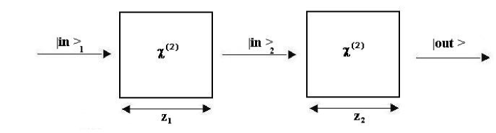
Figure 14: Scheme for a cascade of two $\chi^{(2)}$ nonlinear crystal. The input of the second medium is the output of the first one.

Given a state $|in\rangle_{1}$ at the input of the first crystal, the evolved state $|out\rangle$ at the output of the second crystal is of the form

$$|out\rangle\,=\,e^{-iH_{I}^{(2)}z_{2}}e^{-iH_{I}^{(1)}z_{1}}|in\rangle_{1}\;,$$ (195)

where $H_{I}^{(j)}$ are the interaction Hamiltonians corresponding to the $j$-th crystal, and $z_{j}$ $(j=1,2)$ are the propagation lengths, proportional to the travelling times. This scheme has been proposed by D’Ariano et al. [299] to synthesize the phase-coherent states $|\gamma\rangle=\sqrt{1-|\gamma|^{2}}\sum_{n}\gamma^{n}|n\rangle$, introduced by Shapiro et al. [300]. Each of the processes occurring in the two crystals are described in this case by the three-wave Hamiltonian (86). In the first step, the parametric down-conversion from the vacuum produces a two-mode squeezed vacuum (a so-called twin beam). In the second step, the up-conversion of the twin beam gives origin to the phase coherent states. The two-crystal configuration has also been exploited to engineer macroscopic superpositions [301, 302]. In particular, De Martini has suggested an experimental setup, using two coupled down converter, to generate a field state showing Schrödinger-cat behavior and enhanced entanglement [301].
A suitable multicrystal configuration, including both parametric amplifier and symmetric directional couplers, can realize the multiphoton interaction model

$$H_{I}^{3m}\,=\,\frac{i\dot{r}}{2}\big{[}a_{1}a_{2}+a_{2}a_{3}+a_{3}a_{1}+a_{1}^{{\dagger}}a_{2}+a_{2}^{{\dagger}}a_{3}+a_{3}^{{\dagger}}a_{1}-H.c.\big{]}\;,$$ (196)

where the dot denotes the time derivative, and $\dot{r}/2$ is the coupling. As shown in Ref. [303], the time evolution of an initial vacuum state driven by this Hamiltonian generates the three-mode squeezed vacuum defined as

$$S_{3}|000\rangle\,\equiv\,e^{ir(X_{1}P_{2}+X_{2}P_{3}+X_{3}P_{1})}|000\rangle\;,$$ (197)

where $X_{i}$ and $P_{i}$ are the quadrature operators corresponding to the $i$-th mode. It can be easily proven that $S_{3}$ is a proper squeezing operator for the three-mode quadratures $\tilde{X}=\frac{1}{\sqrt{6}}\sum_{i}X_{i}$ and $\tilde{P}=\frac{1}{\sqrt{6}}\sum_{i}P_{i}$ $([\tilde{X},\tilde{P}]=\frac{i}{2}$). It is evident that the state (197) is a simple generalization of the two-mode squeezed vacuum state $S_{2}|00\rangle=e^{ir(X_{1}P_{2}+X_{2}P_{1})}|00\rangle$, with $r$ real squeezing parameter.
Before ending this Section, we want to mention another recent theoretical development in the realization of multiphoton parametric oscillators [304], again based on the scheme depicted in Fig. (14), but, this time, inserted in a cavity. The model consists of two sequential parametric processes of photon down conversion in $\chi^{(2)}$-nonlinear media placed inside the same cavity, and realizes in principle, by suitably tuning the experimental conditions, the generation either of three-photon, or of four-photon (entangled) states. The quantum statistical properties of these models have been studied by computing the Wigner function resorting to methods of quantum-jump simulations [304, 305, 306]. This study has revealed complete phase-space symmetry for the different arms of the Wigner functions, and multiple stability zones of the subharmonic components. Extensions are obviously possible; in particular, the cascaded frequency doubler generating the second and the fourth harmonics has been recently studied [307].

5 Models of multiphoton interactions and engineering of multiphoton nonclassical states

The many fascinating properties of nonclassical states of light allow, at least in principle, innovative and far-reaching applications in quantum control, metrology, interferometry, quantum information and communication. In a way, although the very concept of nonclassicality presents many subtleties and its quantification is somehow still controversial, one might go so far to say that it should be considered a physical resource to be exploited, much in the same sense as energy and entropy. In Section 2 we have listed some quantities that can be taken as indices of nonclassicality of a state. Among them, we recall the deviation from Poissonian statistics, the Mandel’s $Q$ parameter, the nonexistence of a positive Glauber-Sudarshan $P$ function, and the negativity of the Wigner function. A rich collection of references on nonclassical states in quantum optics has been recently published by Dodonov [308, 309], and a review of optical correlation experiments distinguishing between the predictions of classical and quantum theory can be found in Ref. [310]. In the latter paper, the authors consider an optical field produced by an intracavity four-wave mixing, and discuss the Cauchy-Schwartz and Bell’s inequalities, as well as nonclassical properties as squeezing and antibunching. All these probes of nonclassical behaviors share a common idea: the reference states that are taken as a standard of comparison are the Glauber coherent states, which provide the boundary line of separation between the classical and the quantum domains.
In the previous Section we have reviewed the simplest multiphoton processes arising in nonlinear media, and their ability to generate some standard nonclassical states of light. We have limited our analysis to consolidated experimental settings associated to second- and third-order nonlinearities, and up to four-wave interactions. In this Section we review various methods, models, experimental proposals and realizations, introduced in order to engineer arbitrary nonclassical states of light associated to general multiphoton processes and interactions. A large part of these generalized classes of multiphoton Hamiltonians and multiphoton nonclassical states will be associated to higher-order nonlinearities and will exhibit a great variety of nonclassical properties.

5.1 Nonclassical states by group-theoretical methods

The basic idea of group-theoretical methods is to generalize the concept of coherent state to physical systems with more general symmetries and group-theoretical structures. In this framework, the construction of multiphoton coherent states associated with Lie groups has been carried out by several authors, most notably Klauder [311], Perelomov [312], and Gilmore [313]. The most direct way to construct generalized coherent states is to extend the three Glauber’s original definitions. It is to be remarked, however, that, at variance with the case of the harmonic-oscillator $h_{4}$ algebra, in more general algebraic contexts the three Glauber definitions can define inequivalent classes of states. The simplest procedure is to obtain coherent states as eigenstates of a lowering operator. This approach was used by Barut and Girardello [314] to define a class of generalized coherent states of the group $SU(1,1)$, whose generators $\{K_{+}\,,K_{-}\,,K_{0}\}$ obey the commutation relations (126). As is well known, the group $SU(1,1)$ is associated with the dynamics of the parametric amplifier, in which two photons are created or annihilated. Barut and Girardello thus defined the eigenstates $\{|\varsigma\rangle\}$ of the lowering (or deexcitation) operator $K_{-}$ as the $SU(1,1)$ coherent states:

$$K_{-}|\varsigma\rangle\,=\,\varsigma|\varsigma\rangle\;.$$ (198)

If the group $SU(1,1)$ is in the degenerate realization Eq. (129), for which $K_{-}=\frac{1}{2}a^{2}$, the states $|\varsigma\rangle$ are the cat-like states [315], while if the group is in the nondegenerate realization Eq. (125), for which $K_{-}=ab$, the states $|\varsigma\rangle$ are the pair coherent states [316]. We will discuss these two classes of states in more detail later on. Here we limit ourselves to mention that pair coherent states can be produced by a dissipative dynamics engineered by exploiting the strong competition between four-wave mixing and amplified spontaneous emission in resonant two-photon excitations. These states are deeply entangled and show strong squeezing and antibunching. Extensions of pair coherent states to multimode systems are in principle possible, and have been carried out for three modes (“trio coherent states”) [317]. Generalizations of this approach include the eigenstates of linear combinations of the $SU(1,1)$ operators [318, 319], and the general concept of algebra eigenstates introduced by Brif [320].
A different approach is based on the generalization of minimum uncertainty relations. Given two operators $A$ and $B$ associated to a Lie algebra, minimum uncertainty coherent states are defined as the states that saturate the relation $\Delta A^{2}\Delta B^{2}\geq\frac{1}{4}|\langle[A,B]\rangle|^{2}$ [321, 322, 323, 324]; these states are also known as intelligent states. Both approaches to generalized coherent states, as eigenstates of a lowering operator or as minimum uncertainty states, can be limited in some cases by several constraints, including constraints on the Lie algebra, nonuniqueness of the generalized coherent wave packets, possible nonexistence of a standard resolution of unity.
In fact, the most convenient starting point to construct generalized coherent states is based on the action of a suitable displacement operator on a reference state. Given an algebra with generators $T_{i}$ $(i=1,...,n)$, the generic group coherent state can be defined as

$$|\xi_{1},...,\xi_{n}\rangle\,=\,e^{\sum_{i}\xi_{i}T_{i}}|\Phi_{0}\rangle\;,$$ (199)

where $\xi_{i}$ are complex parameters and $|\Phi_{0}\rangle$ is a fiducial state. To be more specific, we follow Ref. [325], where Zhang, Feng, and Gilmore present a general algorithm for constructing coherent states of dynamical groups for a given quantum physical system. To this aim, let us consider a quantum system described by a certain Hamiltonian expressed in terms of a set of generators $\mathbf{g}\equiv\{T_{i}\}$, spanning a closed algebra, i.e. $[T_{i},T_{j}]=\sum_{k}C_{ij}^{k}T_{k}$, where $C_{ij}^{k}$ are the structure constants of $\mathbf{g}$. The Hamiltonian of the system is typically expressed in linear or quadratic form

$$H\,=\,H(T_{i})\,=\,\sum_{i}c_{i}T_{i}\,+\,\sum_{i,j}c_{ij}T_{i}T_{j}\;.$$ (200)

Let $G$ the dynamical group associated with $\mathbf{g}$. If $\mathbf{g}$ is a semisimple Lie algebra, the operators $\{T_{i}\}$ can be expressed in the standard Cartan basis $\{H_{i}\,,E_{\alpha}\,,E_{-\alpha}\}$ with commutation relations

$$[H_{i},H_{j}]=0\;,$$ (201)

$$[H_{i},E_{\alpha}]=\alpha_{i}E_{\alpha}\;,$$ (202)

$$[E_{\alpha},E_{-\alpha}]=\alpha^{i}H_{i}\;,$$ (203)

$$[E_{\alpha},E_{\beta}]=N_{\alpha,\beta}E_{\alpha+\beta}\;.$$ (204)

The operators $H_{i}$ are diagonal in any unitary irreducible representation $\Gamma^{\Lambda}$ of $G$, and $E_{\alpha}$ are the shift operators. If the representation is Hermitian, we have $H_{i}^{{\dagger}}=H_{i}$ and $E_{\alpha}^{{\dagger}}=E_{-\alpha}$. The first step in the construction of generalized coherent states requires choosing an arbitrary normalized reference state $|\Phi_{0}\rangle$ within the Hilbert space $\mathcal{H}^{\Lambda}$. This reference state will determine the structure of the generalized coherent states and of the phase space of the dynamical system. The maximum stability subgroup $D$ of $G$ is defined as the set of group elements $d$ that leave invariant the reference state $|\Phi_{0}\rangle$ (and will thus depend on the choice of $|\Phi_{0}\rangle$) up to a phase factor:

$$d|\Phi_{0}\rangle\,=\,e^{i\phi(d)}|\Phi_{0}\rangle\;,\;\quad d\in D\;.$$ (205)

Therefore the group $G$ is uniquely decomposed in the two subgroups $D$ and $G/D$ such that

$$\mathbf{g}=\Omega d\;,\;\quad\mathbf{g}\in G\;,\;\quad d\in D\;,\;\quad\Omega\in G/D\;.$$ (206)

Having introduced the complement of $G$ with respect to $D$, the group definition of the generalized coherent states $|\Lambda,\Omega\rangle$ is

$$|\Lambda,\Omega\rangle\,\doteq\,\Omega|\Phi_{0}\rangle\;.$$ (207)

The most useful choice for the reference state $|\Phi_{0}\rangle$ is an unperturbed physical ground state. For this choice the Hamiltonian consists of linear terms in terms of the generators $T_{i}$, and the ground state is an extremal state, defined, at least for Hamiltonians with a discrete spectrum, as the highest-weight state $|\Lambda,\Lambda\rangle$ of the irreducible representation $\Gamma^{\Lambda}$ of the Lie group $G$. Consequently, $E_{\alpha}|\Lambda,\Lambda\rangle=0$, where $\alpha$ belongs to the positive root set of $G$. With this choice, the coset space as well as the generalized coherent states (207) are constructed by the exponential map of shift operators that do not annihilate the extremal state, together with their Hermitian-conjugates. Following this procedure, the generalized coherent states $|\Lambda,\Omega\rangle$ can be written in terms of a displacement operator in one-to-one correspondence to the coset representatives $\Omega$ of $G/D$, acting on the extremal state $|\Lambda,\Lambda\rangle$:

$$\Omega\,=\,\exp\left\{\sum_{\beta}\eta_{\beta}E_{\beta}-\eta_{\beta}^{*}E_{-\beta}\right\}\;,$$ (208)

where $\eta_{\beta}$ are complex parameters, and the sum is restricted to those shift operators which do not annihilate the extremal state. We review the procedure for the trivial case of the harmonic-oscillator coherent states. We know that a single-mode coherent state is realized during the time evolution generated by the one-photon Hamiltonian applied to the initial vacuum:

$$H(t)\,=\,\omega a^{{\dagger}}a\,+\,\kappa(t)a^{{\dagger}}\,+\,\kappa^{*}(t)a\;.$$ (209)

The evolved state is the standard Glauber coherent state (see Section 2). The Hamiltonian (209) is a linear combination of the harmonic oscillator operators $a$, $a^{{\dagger}}$, and $n$, which, together with the identity operator $I$, span the Lie algebra denoted as $h_{4}$; the corresponding Lie group, obtained from the algebra through the operation of exponentiation, is the Heisenberg-Weyl group $H_{4}$. We consider as extremal state the vacuum $|0\rangle$. The stability subgroup which leaves $|0\rangle$ invariant is $U(1)\otimes U(1)$, whose elements take the form $d=e^{i\xi n+i\phi I}$. A representative of the coset space $H(4)/(U(1)\otimes U(1))$ is the Glauber displacement operator $D(\alpha)=e^{\alpha a^{{\dagger}}-\alpha^{*}a}$. Therefore the Glauber coherent states can be obtained by the action on the extremal state $|0\rangle$ of the element $\mathbf{g}\in H_{4}$, $\mathbf{g}=D(\alpha)d$:

$$\mathbf{g}|0\rangle\,=\,D(\alpha)d|0\rangle\,=\,e^{i\phi}|\alpha\rangle\;.$$ (210)

Another simple case of generalized coherent state is the single-mode squeezed state that is generated during the time evolution driven by the positive definite quadratic Hamiltonian (153) which is a linear combination of the operators spanning the algebra $h_{6}=\left\{n,a,a^{{\dagger}},a^{2},a^{{\dagger}2},I\right\}$, a subalgebra of the symplectic algebra $sp(4)$. The evolution operator can be disentangled by using the equivalent matrix representations of the group $H_{6}$. In analogy with the case of the Heisenberg-Weyl group, the coherent states of $H_{6}$ are obtained by choosing the vacuum state as extremal state, and by considering a representative in the coset space $H_{6}/(U(1)\otimes U(1))$, that is the product $D(\alpha)S(\varepsilon)$ of the displacement and squeezing operators. The single-mode algebra $h_{6}$ can be extended to the $n$-mode case [325], by considering the subgroup of $sp(2n+2)$, generated by the operators $\left\{a_{i}^{{\dagger}}a_{j}^{{\dagger}},a_{i}^{{\dagger}}a_{j}+\frac{1}{2}\delta_{ij},a_{i}a_{j},a_{i}^{{\dagger}},a_{j},I\right\}$, which are the independent elements needed to construct the multimode generalization of Hamiltonian (153):

$$H\, =\,\sum_{i}\omega_{i}\left(a^{{\dagger}}_{i}a_{i}+\frac{1}{2}\right)+\sum_{ij}(p_{ij}\,a_{i}^{{\dagger}}a_{j}^{{\dagger}}+h.c.)$$ (211)

$$+\sum_{ij}r_{ij}\left(a_{i}^{{\dagger}}a_{j}+\frac{1}{2}\delta_{ij}\right)+\sum_{i}(s_{i}a^{{\dagger}}_{i}+h.c.)\;.$$

More recently, the formalism of nonlinear algebras has been applied to multiphoton optical Hamiltonians associated to symmetries which can be described by polynomially deformed $SU(1,1)$ and $SU(2)$ algebras [326]. A general approach to construct the multiphoton coherent states of such algebras has been introduced in Ref. [327]. Here we want to briefly recall the basic concepts of this method. In the Cartan basis, a deformation of a Lie algebra is obtained by replacing Eq. (203) with $[E_{\alpha},E_{-\alpha}]=f(H_{i})$, where $f(H_{i})$ is a polynomial function of $H_{i}$. In particular, the polynomial deformation of the Jordan-Schwinger realizations of the $SU(2)$ and $SU(1,1)$ algebras takes the form

$$[J_{0},J_{\pm}]\,=\,\pm J_{\pm}\;,\;\quad[J_{+},J_{-}]\,=\,F(J_{0})\,=\,\sum_{i=0}^{n}C_{i}J_{0}^{i}\;,$$ (212)

where $J_{0}$ is the diagonal operator, $J_{\pm}$ are the scaling operators, and the coefficients $C_{i}$ are real constants. Interesting cases are the quadratic algebra ($F(J_{0})$ quadratic in $J_{0}$) and the cubic, or Higgs, algebra ($F(J_{0})$ cubic in $J_{0}$). For example, the coherent states associated with the trilinear Hamiltonian (124) have been defined by using the generators of the polynomial quadratic algebra, $J_{0}=\frac{1}{2}(a^{{\dagger}}a-K_{0})$, $J_{+}=a^{{\dagger}}K_{-}=J_{-}^{{\dagger}}$ [327]. The spectrum and the eigenfunctions of the general two-mode multiphoton Hamiltonian

$$H_{Hig}\,=\,\omega_{1}a_{1}^{{\dagger}}a_{1}+\omega_{2}a_{2}^{{\dagger}}a_{2}+\kappa a_{1}^{{\dagger}2}a_{2}^{2}+\kappa^{*}a_{1}^{2}a_{2}^{{\dagger}2}\;,$$ (213)

can be found [328] by exploiting the Higgs algebra, generated by the operators $J_{+}=a_{1}^{{\dagger}2}a_{2}^{2}=J_{-}^{{\dagger}}$, and $J_{0}=\frac{1}{4}(a_{1}^{{\dagger}}a_{1}-a_{2}^{{\dagger}}a_{2})$.
Another class of nonlinear coherent and squeezed states associated with a simple nonlinear extension of the harmonic-oscillator algebra can be obtained as follows. Given a well defined, Hermitian function $f(n)$ of the number operator $n$, let us define the pair of lowering and raising operators

$$A\,=\,af(n)\;,\;\quad A^{{\dagger}}\,=\,f(n)a^{{\dagger}}\;,$$ (214)

which satisfy the following commutation relations

$$[n,A]=-A\;,\;\quad[n,A^{{\dagger}}]=A^{{\dagger}}\;,$$

$$[A,A^{{\dagger}}]\,=\,(n+1)f(n+1)^{2}-nf(n)^{2}\;.$$ (215)

Nonlinear coherent and squeezed states can be constructed either as eigenstates of the generalized annihilation operator $A$ [329, 330], namely

$$A|\gamma,f\rangle\,=\,af(n)|\gamma,f\rangle\,=\,\gamma|\gamma,f\rangle\;,$$ (216)

or by the action of a displacement-type operator on the vacuum [331, 332]. In this case, we first need the definition of a dual algebra by defining the canonical conjugate $B^{{\dagger}}$ of $A$:

$$B^{{\dagger}}\,\doteq\,\frac{1}{f(n)}a^{{\dagger}}\;,\;\;\quad[A,B^{{\dagger}}]=1\;.$$ (217)

Nonlinear coherent and squeezed states are then defined as

$$|\zeta,f\rangle\,=\,e^{\zeta A^{{\dagger}}-\zeta^{*}B}|0\rangle\;,\;\;\quad|\tilde{\zeta},f\rangle\,=\,e^{\tilde{\zeta}B^{{\dagger}}-\tilde{\zeta}^{*}A}|0\rangle\;,$$ (218)

$$|\xi,f\rangle\,=\,e^{\frac{1}{2}(\xi A^{{\dagger}2}-\xi^{*}B^{2})}|0\rangle\;,\;\;\quad|\tilde{\xi},f\rangle\,=\,e^{\frac{1}{2}(\tilde{\xi}B^{{\dagger}2}-\tilde{\xi}^{*}A^{2})}|0\rangle\;.$$ (219)

An extension of this approach that yields a larger class of multiphoton coherent state was formulated by Shanta, Chaturvedi, Srinivasan, and Agarwal [333]. They developed a method to derive the eigenstates of a generalized (multiphoton) annihilation operator $F$ consisting of products of annihilation operators and of functions of the number operators. The method is based on constructing a family of operators $\{G_{i}^{{\dagger}}\}$ such that $[F,G_{i}^{{\dagger}}]=1$. Let $|v\rangle_{i}$, $i=0,1,...$, denote the states annihilated by $F$, and let $\{S_{i}\}$ the collection of subspaces of states realized by repeated application of the operator $F^{{\dagger}}$ on $|v\rangle_{i}$. The Fock space is then decomposed into the mutually orthogonal sectors $S_{i}$. Let $G_{i}^{{\dagger}}$ be an operator such that $[F,G_{i}^{{\dagger}}]=1$ holds in the sector $S_{i}$. The conjugate $G_{i}$ annihilates the same states as $F$: $G_{i}|v\rangle_{i}=0$ $\forall$ $i$. The following states

$$|f\rangle_{i}\,=\,e^{fG_{i}^{{\dagger}}}|v\rangle_{i}\;,\;\;\quad|g\rangle_{i}\,=\,e^{gF^{{\dagger}}}|v\rangle_{i}$$ (220)

are eigenstates of $F$ and $G_{i}$, respectively, i.e. $F|f\rangle_{i}=f|f\rangle_{i}$ and $G_{i}|g\rangle_{i}=g|g\rangle_{i}$, and they satisfy the relation ${}_{i}\langle f|g\rangle_{k}=e^{f^{*}g}\delta_{ik}$. For simplicity, we consider the single-mode case with $F$ of the form $f(a^{{\dagger}}a)a^{p}$ (with $f(x)\neq 0$ at $x=0$ and at positive integer values of $x$). The vacua $|v\rangle_{i}$ coincide with the Fock states $|i\rangle$, $i=0,1,...,(p-1)$, and the sectors $S_{i}$ are built out of these vacua by repeated applications of $F^{{\dagger}}$: $S_{i}=\{|pn+i\rangle\}$, ($n=0,1,...$). The operators $G_{i}^{{\dagger}}$ can be explicitly constructed

$$G_{i}^{{\dagger}}\, = \,\frac{1}{p}[a^{{\dagger}}a-i]F^{{\dagger}}\frac{1}{FF^{{\dagger}}}$$ (221)

$$= \,\frac{1}{p}F^{{\dagger}}\frac{1}{FF^{{\dagger}}}[a^{{\dagger}}a+p-i]\,=\,G_{0}^{{\dagger}}\frac{a^{{\dagger}}a+p-i}{a^{{\dagger}}a+p}\;.$$

A clarifying example is obtained in the particular case $F=a^{2}$ $(f=1\,,\;\;p=2)$. The two vacua of $F$ are the states $|0\rangle$ and $|1\rangle$ and the corresponding sectors of the Fock space are $S_{0}=\{|2n\rangle\}_{n=0}^{\infty}$ and $S_{1}=\{|2n+1\rangle\}_{n=0}^{\infty}$, respectively, the sets of even and odd number states. The canonical conjugates of $F$ in the two sectors are

$$G_{0}^{{\dagger}}\,=\,\frac{1}{2}a^{{\dagger}2}I_{a}\;,\;\;\quad G_{1}^{{\dagger}}\,=\,\frac{1}{2}a^{{\dagger}}I_{a}a^{{\dagger}}\;,$$ (222)

where $I_{a}=\frac{1}{1+a^{{\dagger}}a}$. Consequently, the eigenstates of $F$ are

$$|f\rangle_{0}\,=\,e^{\frac{f}{2}a^{{\dagger}2}I_{a}}|0\rangle\;,\;\;\quad|f\rangle_{1}\,=\,e^{\frac{f}{2}a^{{\dagger}}I_{a}a^{{\dagger}}}|1\rangle\;,$$ (223)

namely, linear combinations of the even and odd Fock states, respectively. The corresponding eigenstates of $G_{0}$ and $G_{1}$ are

$$|g\rangle_{0}\,=\,e^{ga^{{\dagger}2}}|0\rangle\;,\;\;\quad|g\rangle_{1}\,=\,e^{ga^{{\dagger}2}}|1\rangle\;.$$ (224)

The state $|g\rangle_{0}$ with $|g|\leq 1$ is the squeezed vacuum, while $|g\rangle_{1}$ is a squeezed number state. This scheme allows for a systematic construction of the eigenstates of products of annihilation operators.

5.2 Hamiltonian models of higher-order nonlinear processes

We will now introduce the study of phenomenological theories of $k$-photon parametric amplification, for arbitrary $k$, based on the quantization of expression (78) [221, 222, 223, 224, 225, 226, 227, 334, 335, 336, 337, 338, 339].

5.2.1 Nondegenerate, fully quantized $k$-photon down conversion

Already in 1984, a dissipative multimode parametric amplifier was studied by Graham [340] to derive a general relation between the intensity cross-correlation function and the intensity autocorrelations for any pair of simultaneously excited modes. The nondegenerate, $k$-photon parametric amplifier is described by the interaction Hamiltonian of the general form

$$H_{I}^{ndg,kph}\,=\,\kappa^{(k)}a_{1}^{{\dagger}}a_{2}^{{\dagger}}\cdots a_{k}^{{\dagger}}b\,+\,H.c.\;,$$ (225)

with real $\kappa^{(k)}$ and under condition of approximate resonance $|\omega_{b}-\sum_{i=1}^{k}\omega_{i}|\ll\omega_{j}$, $j=1,\ldots,k$. In the absence of losses, by using the conserved quantities $D_{ij}=a_{i}^{{\dagger}}a_{i}-a_{j}^{{\dagger}}a_{j}$, it can be shown that the intensities of pairs of excited modes are maximally correlated at all times, namely $\langle a_{i}^{{\dagger}}a_{i}\rangle=\langle a_{j}^{{\dagger}}a_{j}\rangle$ and $\langle a_{i}^{{\dagger}}a_{j}^{{\dagger}}a_{i}a_{j}\rangle=\langle a_{i}^{{\dagger}}a_{i}^{{\dagger}}a_{i}a_{i}\rangle+\langle a_{i}^{{\dagger}}a_{i}\rangle$ $(i\neq j)$. If finite losses are considered, solution of the master equation in the steady state yields

$$\eta_{i}\langle a_{i}^{{\dagger}}a_{i}\rangle\, = \,\eta_{j}\langle a_{j}^{{\dagger}}a_{j}\rangle$$ (226)

$$\langle a_{i}^{{\dagger}}a_{j}^{{\dagger}}a_{i}a_{j}\rangle\, = \,\frac{\eta_{i}}{\eta_{i}+\eta_{j}}\langle a_{i}^{{\dagger}}a_{i}^{{\dagger}}a_{i}a_{i}\rangle+\frac{\eta_{j}}{\eta_{i}+\eta_{j}}\langle a_{j}^{{\dagger}}a_{j}^{{\dagger}}a_{j}a_{j}\rangle$$ (227)

$$+ \frac{\eta_{i}}{\eta_{i}+\eta_{j}}\langle a_{i}^{{\dagger}}a_{i}\rangle\,,\quad\quad i\neq j\,,$$

where $\eta_{i}$ is a phenomenological constant relative to the mode $a_{i}$. Since the total power $P_{i}$ extracted from the mode $a_{i}$ is given by $P_{i}=2\eta_{i}\omega_{i}\langle a_{i}^{{\dagger}}a_{i}\rangle$, Eq. (226) implies the Manley-Rowe’s relation [162]

$$\frac{P_{1}}{\omega_{1}}\,=\,\frac{P_{2}}{\omega_{2}}\,=\,\ldots\,\frac{P_{k}}{\omega_{k}}\;.$$ (228)

Eqs. (227) show the presence of strong correlations between excited modes due their joint, simultaneous generation by the same quantum process. It is quite evident that, for reasons of convenience and practicality, most of the studies are devoted to the simplest case of complete degeneracy, described by the Hamiltonian

$$H_{I}^{dg,kph}\,=\,\kappa^{(k)}a^{{\dagger}k}b\,+\,H.c.\;,$$ (229)

where $\kappa^{(k)}$ is proportional to the $k$-th order nonlinearity. After these preliminary considerations on the most general, nondegenerate, fully quantized $k$-photon interaction, in the following we will review more in detail the approaches and the methods used to study the dynamics of the degenerate $k$-photon amplifier, either in the fully quantized version or in the parametric approximation for the pump mode.

5.2.2 Degenerate $k$-photon down conversion with classical pump

In 1984, Fisher, Nieto, and Sandberg [221] claimed the impossibility of generalizing the squeezed coherent states by means of generalized $k$-photon ($k>2$), unitary “squeezing” operators of the form:

$$U_{k}\,=\,\exp\{iA_{k}\}\,=\,\exp\{z_{k}a^{{\dagger}k}\,-\,z_{k}^{*}a^{k}+\,ih_{k-1}\}\;,\;\;\;k>2\;,$$ (230)

where $h_{q}$ is a Hermitian operator polynomial in $a$ and $a^{{\dagger}}$ with degree $q$. In particular, they considered the vacuum expectation value of $U_{k}$ with $h_{q}=0$ and showed that this operator is unbounded. In fact, expanding the exponential of Eq. (230) in a power series and taking the expectation value in the vacuum state, it results

$$\langle 0|U_{k}|0\rangle\, = \,1-|z_{k}|^{2}\frac{k!}{2!}+|z_{k}|^{4}\frac{1}{4!}[(k!)^{2}+(2k)!]$$ (231)

$$+ ...+(-1)^{n}|z_{k}|^{2n}\frac{1}{(2n)!}C_{n}+...\;,$$

where $C_{n}$ is formed of positive terms.
The largest one is of order $(kn)!$, so that $\lim_{n\rightarrow\infty}|z_{k}|^{2n}\frac{1}{(2n)!}C_{n}\neq 0$ for all $k>2$ and $z_{k}\neq 0$. The terms of large order $2n$ in the series with alternating signs (231) are bounded from below by $(kn)!/(2n)!$, which has no convergent limit for $n\rightarrow\infty$ when $k>2$. In conclusion, the series is divergent, and $|0\rangle$ is not an analytic vector of the generator $A_{k}$ in the Fock space. Therefore, a ”naive” generalization of one-photon coherent states and two-photon squeezed states to many-photon generalized squeezed and coherent states appears to be impossible.

The problem raised in Ref. [221] inspired the introduction of new types of generalized $k$-photon squeezed coherent states [334, 335], whose definition is based on the generalized multiphoton operators of Brandt and Greenberg [163], including those defined for Holstein-Primakoff realizations [341] of $SU(2)$, $SU(1,1)$ and $SU(n)$ [335].
However, the problem of the divergence of the vacuum to vacuum matrix element (231) can be approached by more standard methods, and has in fact been solved by Braunstein and McLachlan [222]. They studied the matrix element by numerical techniques and, using Padé approximants, obtained good convergence of the asymptotic series. They considered the degenerate multiphoton parametric amplifier (229) that, in the Schrödinger picture, for $k$-photon processes, and within the parametric approximation takes the form

$$H_{P}^{dg,kph}\,=\,\omega a^{{\dagger}}a\,+\,i[z_{k}(t)a^{{\dagger}k}-z_{k}^{*}(t)a^{k}]\;,$$ (232)

where $z_{k}(t)=|z|e^{i(\phi-k\omega t)}$. In the interaction picture, the time evolution operator corresponding to Eq. (232) reads

$$U_{k}(z,z^{*};t)\,=\,\exp\{(za^{{\dagger}k}-z^{*}a^{k})t\}\;,$$ (233)

where $z=|z|e^{i\phi}$. The properties of the states generated by the time evolution Eq. (233) can be studied using the Husimi function $Q(\alpha)=Tr[\rho(t)\delta(a-\alpha)\delta(a^{{\dagger}}-\alpha^{*})]$, where $\rho(t)=U_{k}(t)\rho(0)U_{k}^{{\dagger}}(t)$. If the initial state is the vacuum $\rho(0)=|0\rangle\langle 0|$, $Q$ is invariant under a rotation of $2\pi/k$, leading to a $k$-fold symmetry in phase space. Assuming a real $z$, defining a scaled time $r=|z|t$, and exploiting the equations of motion for the density operator in the interaction picture and standard operatorial relations, the evolution equation for the $Q-$function reads

$$\frac{\partial Q}{\partial r}\,=\,LQ\,\equiv\,\left\{\alpha^{k}-\left(\alpha+\frac{\partial}{\partial\alpha^{*}}\right)^{k}+\alpha^{*k}-\left(\alpha^{*}+\frac{\partial}{\partial\alpha}\right)^{k}\right\}Q\;,$$ (234)

where $L$ is the Liouvillian operator. The general solution of Eq. (234) is of the form

$$Q(r)\,=\,\exp\{rL\}Q(0)\,=\,Q(0)\,+\,LQ(0)r\,+\,\frac{1}{2}L^{2}Q(0)r^{2}\,+\,...\;,$$ (235)

where $Q(0)$ is the initial value of the $Q-$function. Being that the series (235) is in fact asymptotic, it can be truncated in order to determine the small-time behavior. For the initial vacuum state $\rho(0)=|0\rangle\langle 0|$, this truncation yields

$$Q(r)\, \sim \,e^{-|\alpha|^{2}}[1+r(\alpha^{k}+\alpha^{*k})]\,+\,\mathcal{O}(r^{2})$$ (236)

$$= \,e^{-|\alpha|^{2}}[1+2r|\alpha|^{k}\cos(k\theta)]\,+\,\mathcal{O}(r^{2})\;,$$

where $\alpha=|\alpha|e^{i\theta}$. For $r\ll 1$ the $Q-$function exhibits $k$ lobes along the directions $\theta=0,\frac{2\pi}{k},...,\frac{2\pi(k-1)}{k}$, showing a strong nonclassical behavior even for short times. In Fig. (15) we show contour-plots of the $Q$-function corresponding to $U_{3}$ and $U_{4}$, with $r=0.1$ and $r=0.025$ respectively; the presence of the arms, revealing the symmetry of the system, can be observed already for short times.

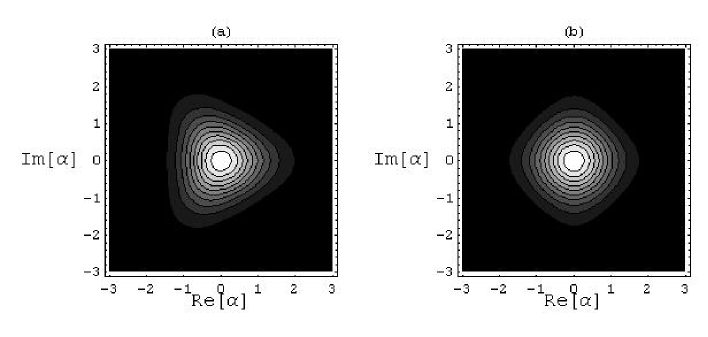
Figure 15: Contour plots of the $Q$-function for the initial vacuum state and for $(a)$ $k=3$, $r=0.1$; $(b)$ $k=4$, $r=0.025$.

There is no analytic technique to study the full dynamics at all times; one possible method is to expand the $Q$-function in a power series in terms of Fock space matrix elements of the evolution operator:

$$Q(r)\,=\,\exp\{-|\alpha|^{2}\}\left|\sum_{n=0}^{\infty}\frac{\alpha^{*n}}{\sqrt{n!}}\langle n|U_{k}(r)|0\rangle\right|^{2}\;.$$ (237)

The problem is then further reduced because the matrix elements are nonvanishing only for $n$ multiple of $k$, $n=mk$. In this case one has

$$\langle k|U_{k}(r)|0\rangle=\frac{1}{\sqrt{k!}}\frac{d}{dr}\langle 0|U_{k}(r)|0\rangle\,,$$

$$\langle 2k|U_{k}(r)|0\rangle=\frac{1}{\sqrt{(2k)!}}\left(k!+\frac{d^{2}}{dr^{2}}\right)\langle 0|U_{k}(r)|0\rangle\,,\;....\,.$$ (238)

The divergence of the vacuum-to-vacuum matrix element is due to the singular behavior on the imaginary time axis, since the Taylor series converges only up to the nearest pole. An analytic continuation can be obtained using the Padé approximants [342] which reproduce the pole structure that limits the convergence of the Taylor series. Therefore, one can conclude, following Braunstein and McLachlan, that the generalization of one-photon coherent states and two-photon squeezed states to the many-photon case is possible, and that the resulting non Gaussian states show evident nonclassical features.
Successively, Braunstein and Caves [223] have studied in detail the statistics of direct, heterodyne and homodyne detection for the generalized squeezed states associated with the cubic and quartic interaction Hamiltonians

$$H_{P}^{dg,3ph} = i\kappa(a^{{\dagger}3}-a^{3})\;,$$ (239)

$$H_{P}^{dg,4ph} = i\kappa(a^{{\dagger}4}-a^{4})\;,$$ (240)

($\kappa$ real), and to the interaction Hamiltonian introduced by Tombesi and Mecozzi [336]

$$H_{P}^{dg,(2-2)ph}\,=\,\kappa[i(a^{{\dagger}2}-a^{2})]^{2}\,=\,-\kappa(a^{{\dagger}4}+a^{4})\,+\,\kappa(a^{{\dagger}2}a^{2}+a^{2}a^{{\dagger}2})\;.$$ (241)

The Hamiltonians $H_{P}^{dg,3ph}$ and $H_{P}^{dg,4ph}$ can be studied by numerical methods, while the Hamiltonian $H_{P}^{dg,(2-2)ph}$ describes an exactly solvable model [336] based on both four-photon and Kerr processes in nonlinear crystals without inversion center. It can be obtained by the model Hamiltonian

$$H_{M}\,=\,\omega a^{{\dagger}}a+\gamma^{(3)}(a^{{\dagger}2}a^{2}+a^{2}a^{{\dagger}2})+\gamma^{(4)}[E^{*}(t)a^{4}+E(t)a^{{\dagger}4}]\;,$$ (242)

where $\gamma^{(3)}$ and $\gamma^{(4)}$ are proportional, respectively, to the third- and fourth-order susceptibility tensors, and $E(t)=Ee^{i\phi-4\omega t}$ is a classical external pump field. In the interaction picture, setting the phase of the pump $\phi=\pi$ and choosing the amplitude $E$ such that $E=\gamma^{(3)}/\gamma^{(4)}$, the Hamiltonian (242) leads to Eq. (241), defining $\kappa=\gamma^{(4)}E$. The time evolution operators corresponding to the Hamiltonians of Eqs. (239), (240) and (241) are respectively

$$U_{3}(r)\,=\,e^{r(a^{{\dagger}3}-a^{3})}\;,$$ (243)

$$U_{4}(r)\,=\,e^{r(a^{{\dagger}4}-a^{4})}\;,$$ (244)

$$U_{2,2}(r)\,=\,e^{ir(a^{{\dagger}2}-a^{2})^{2}}\;,$$ (245)

where $r=\kappa t$ is a scaled time. The evolution operator $U_{2,2}(r)$ can be written as a Gaussian average over the analytic continuation of the quadratic evolution operator [336]

$$U_{2,2}(r)\,=\,\int_{-\infty}^{\infty}d\xi\frac{1}{\sqrt{\pi}}e^{-\xi^{2}}e^{2\sqrt{ir}\xi(a^{{\dagger}2}-a^{2})}\;.$$ (246)

In this case, the vacuum-to-number-state matrix elements are given by

$$\langle n|U_{2,2}(r)|0\rangle=$$

$$\pi^{-1/2}\sqrt{n!}[(n/2)!]^{-1}2^{-n/2}\int_{-\infty}^{\infty}d\xi e^{-\xi^{2}}\frac{\left(\tanh\tau\right)^{n/2}}{\left(\sqrt{\cosh\tau}\right)}\left|{}_{\tau=4\sqrt{ir\xi}}\right.\quad n\;even,$$ (247)

and $0$ for $n$ odd. The statistics of direct, heterodyne, and homodyne detection correspond, respectively, to determine the photon number distribution, the $Q$-function, and the projections of the Wigner function [223]. For the Hamiltonian $H_{P}^{dg,3ph}$, the photon number distribution shows photon triplets, while for $H_{P}^{dg,4ph}$ and $H_{P}^{dg,(2-2)ph}$ it shows photon quadruplets. In the same way, the $Q$-function exhibits the characteristic shape with three and four arms (lobes). Finally, the Wigner function shows interference fringes due to coherent superposition effects in phase space.

5.2.3 Degenerate $k-$photon down-conversion with quantized pump

We now turn to the properties of $k-$photon down-conversion with quantized pump in a high-Q cavity in the presence of a Kerr-like medium. Among others, the collapses and revival phenomenon in the energy exchange of two field modes [225], the statistics of the process [226], the phase properties [227], the signal-pump entanglement [339], and the limit on the energy transfer between the modes [339] have been studied. In the rotating wave approximation, the process of $k-$photon down conversion, with $k\geq 3$, can be described, including the free parts and the Kerr terms, by the effective total Hamiltonian

$$H_{Q}^{dg,kph}\, = \,\omega_{a}a^{{\dagger}}a+\omega_{b}b^{{\dagger}}b+\lambda_{k}(a^{k}b^{{\dagger}}+a^{{\dagger}k}b)$$ (248)

$$+ g_{a}a^{{\dagger}2}a^{2}+g_{b}b^{{\dagger}2}b^{2}+g_{ab}a^{{\dagger}}ab^{{\dagger}}b\;,$$

where exact resonance $\omega_{b}=k\omega_{a}$ is assumed, and $\lambda_{k}$, $g_{a}$, and $g_{b}$ are real constants, with $\lambda_{k}\propto\chi^{(k)}$, and the $g_{i}s\propto\chi^{(3)}$. The time evolution generated by Hamiltonian (248) is not plagued by the divergences that appear in the parametric approximation studied in the previous paragraph. The integral of motion

$$N^{(k)}\,=\,a^{{\dagger}}a\,+\,kb^{{\dagger}}b$$ (249)

decomposes the Hilbert space of the whole system $\mathcal{H}=\mathcal{H}_{a}\otimes\mathcal{H}_{b}$ in the direct sum $\mathcal{H}=\oplus_{i}\mathcal{H}_{i}$, where each subspace $\mathcal{H}_{i}$, associated to a fixed, positive integer value $N_{i}$ ($N_{i}=0,...,\infty$) of $N^{(k)}$, is defined as the set of all state vectors that can be expressed as linear combinations of the basis vectors $\{|N_{i}-nk,n\rangle\;,n=0,...,[N_{i}/k]\}$, where $|N_{i}-nk,n\rangle$ is a compact notation for the two-mode number state $|N_{i}-nk\rangle_{a}|n\rangle_{b}$, and $[x]$ stands for the integer part of $x$. The dimension of the subspace $\mathcal{H}_{i}$ is $[N_{i}/k]+1$. This decomposition of the Hilbert space enables to diagonalize the Hamiltonian on each subspace $\mathcal{H}_{i}$, with eigenvalue equation

$$H_{Q}^{dg,kph}|\Psi_{\gamma,N_{i}}\rangle\,=\,E_{\gamma,N_{i}}|\Psi_{\gamma,N_{i}}\rangle\;,$$ (250)

where $\gamma=0,...,[N_{i}/k]$. In terms of the eigenvalues and eigenvectors, the evolution operator of the system can be written in the form

$$U(t)\,=\,e^{-itH_{Q}^{dg,kph}}\,=\,\sum_{N_{i}=0}^{\infty}\sum_{\gamma=0}^{[N_{i}/k]}e^{-itE_{\gamma,N_{i}}}|\Psi_{\gamma,N_{i}}\rangle\langle\Psi_{\gamma,N_{i}}|\;,$$ (251)

and the eigenstates $|\Psi_{\gamma,N_{i}}\rangle$ can be expressed in the basis $\{|N_{i}-nk,n\rangle\}$ as

$$|\Psi_{\gamma,N_{i}}\rangle\,=\,\sum_{m=0}^{[N_{i}/k]}\langle N_{i}-mk,n|\phi_{\gamma,N_{i}}\rangle|N_{i}-mk,n\rangle\;,$$ (252)

so that, finally, given any initial state $|\Phi\rangle_{0}$ of the system, it is possible to reconstruct the density matrix $\rho(t)$ and to analyze the statistical properties of the field at all times. In the following analysis, all the Kerr terms in the Hamiltonian (248) will be put to zero for simplicity. On the other hand, this choice will be physically justified a posteriori in the case $k=3$ (possibly resonant). Moreover, concerning the mathematical analysis of the problem with generic $k$, such terms are harmless because they always commute with the integral of motion $N^{(k)}$. Clearly, a convenient choice for $|\Phi\rangle_{0}$ is the pure two-mode Fock state $|N_{i}-kl,l\rangle$; however, a more realistic choice is the state $|0\rangle_{a}|\beta\rangle_{b}$. Every initial state $|\Phi\rangle_{0}$ can be expressed as $|\Phi\rangle_{0}=\sum_{N_{i}=0}^{\infty}c_{N_{i}}|\Phi_{N_{i}}\rangle_{0}$, where $|\Phi_{N_{i}}\rangle_{0}$ is the normalized projection of the initial state on the subspace associated to the value $N_{i}$ of the integral of motion, and with real weight factor $c_{N_{i}}$ ($\sum_{N_{i}=0}^{\infty}c_{N_{i}}^{2}=1$). It is worth noting that the form of the initial state will strongly influence the dynamics of the system. As a simple example, we will study the time evolution driven by the three-photon down conversion ($k=3$) Hamiltonian (248), without Kerr-like terms, of the initial Fock state $|\Phi\rangle_{0}=|4,7\rangle$, and thus with a constant of motion $N_{i}=25$. In Fig. (16) we show the time evolution of the mean intensity $I_{j}(\tau)$ $(j=a,b)$ in the two modes as a function of the scaled, dimensionless time $\tau=\lambda_{3}t$.

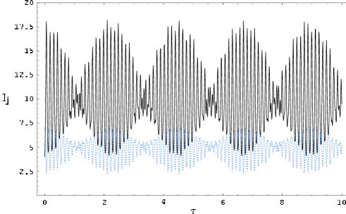
Figure 16: $I_{j}(\tau)$ as a function of the dimensionless time $\tau$ for an initial Fock state $|4,7\rangle$, nonlinearity of order $k=3$, and constant of the motion $N_{i}=25$. The upper curve (full line) corresponds to $I_{a}(\tau)$ in the degenerate mode $a$; the lower curve (dotted line) corresponds to $I_{b}(\tau)$ in the quantized pump mode $b$. The beats’ envelope and the sequence of collapses and revivals are clearly observable.

A very sharp sequence of collapses and revivals in the energy exchange between the field and the pump modes is clearly observable. The introduction of the Kerr terms can lead to an enhancement of the phenomenon; on the other hand, for too high values of the Kerr couplings $g_{i}$, the collapse-revival behavior is lost and replaced by a modulated oscillatory behavior. To establish the statistical properties of the fields, we can evaluate the Mandel’s $Q$ parameter. Fig. (17) (a) shows the evolution of the $Q$ parameter for the same initial Fock state. We see that the pump mode $b$ exhibits strong oscillations between the super-Poissonian (positive $Q$) and the sub-Poissonian regime (negative $Q$), while the statistics of mode $a$, although presenting fast oscillations, remains almost always super-Poissonian.

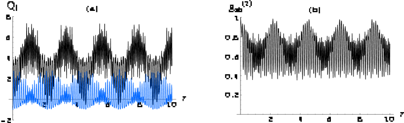
Figure 17: Figure (a): $Q$ parameters of mode $a$ and mode $b$ as functions of the rescaled, dimensionless time $\tau$ for the initial Fock state $|4,7\rangle$, $k=3$, and $N_{i}=25$. The upper curve (full line) corresponds to $Q_{a}(\tau)$, the lower (dotted line) to $Q_{b}(\tau)$. Strong oscillations between super- and sub-Poissonian statistics in mode $b$ are clearly observable. Figure (b): Cross-correlation $g^{(2)}_{ab}$ as a function of the rescaled, dimensionless time $\tau$, for the same initial state. Anticorrelation of the modes is observed at all times.

However, it can be shown that for small values of $N_{i}$ the statistics in both modes remains almost always sub-Poissonian, while for increasing $N_{i}$ the statistics tends to lose its sub-Poissonian character in either mode. Another interesting physical feature can be investigated through the time evolution of the cross-correlation function $g_{ab}^{(2)}=\langle a^{{\dagger}}ab^{{\dagger}}b\rangle/\langle a^{{\dagger}}a\rangle\langle b^{{\dagger}}b\rangle$. As shown in Fig. (17) (b), $g_{ab}^{(2)}<1$ at all times, indicating a permanent anticorrelation of the field and pump modes, so that there is a strong tendency for photons in the two different modes not to be created/detected simultaneously. When $|\Phi\rangle_{0}=|0\rangle_{a}|\beta\rangle_{b}$ and the intensity $|\beta|$ of the initial coherent state for mode $b$ is high enough, the anticorrelation can be violated [226]. The quantum dynamics realized by the Hamiltonian (248) is also able to produce strong entangled states of the signal and pump modes. To quantify quantum correlations in a two-mode pure state (and, in general, in any bipartite pure state) we can resort to the von Neumann entropy of the reduced single-mode mixed state of any of the two modes: $S^{(\alpha)}=-Tr_{\alpha}[\rho_{\alpha}\ln\rho_{\alpha}]$, where $\rho_{\alpha}=Tr_{\alpha^{\prime}\neq\alpha}[\rho]$ is the reduced density operator for mode $\alpha$ ($\alpha=a,b$). If the two modes are assumed to be initially in a pure product state, then $S^{(a)}(t=0)=S^{(b)}(t=0)=0$. As the evolution is unitary (Hamiltonian), the total entropy $S$ of the system is a conserved quantity. From the Araki-Lieb theorem [343], which can be expressed in the form $|S^{(a)}-S^{(b)}|\leq S\leq S^{(a)}+S^{(b)}$, it follows that $S(t)=0$ and $S^{(a)}=S^{(b)}$ for any $t>0$. An equivalent measure of entanglement for pure bipartite states is the reduced linear entropy $S_{L}$, that, for simplicity, we will use in the following, defined as:

$$S_{L}\,=\,1-Tr_{a}[\rho_{a}^{2}]\,=\,1-Tr_{b}[\rho_{b}^{2}]\;,$$ (253)

where $Tr[\rho^{2}]$ measures the purity of a state: $Tr[\rho^{2}]\leq 1$, and saturation is reached only for pure states. The linear entropy is in fact a lower bound to the von Neumann entropy: $S_{L}\leq S^{(\alpha)}$, so that the higher $S_{L}$, the higher is the entanglement between the pump and the signal mode. In Fig. (18) we plot the time evolution of the linear entropy $S_{L}$ during the process of three-photon down conversion, starting from the initial, factorized Fock state $|4,7\rangle$.

Figure 18: Linear entropy $S_{L}$ as a function of the scaled, dimensionless time $\tau$ for the initial factorized two-mode Fock state $|4,7\rangle$, and nonlinearity of order $k=3$. The entanglement is highly oscillatory, but remains finite at all times $\tau>0$.

We see that the Hamiltonian (248) has a strong entangling power, and, as long as the interaction stays on, the entanglement remains nonvanishing at all times, although exhibiting a fast oscillatory behavior. More generally, for an initial coherent state of the pump mode, the entanglement is an increasing function both of the order of the process and of the intensity of the pump [338].
We conclude this short discussion of multiphoton down conversion processes with fully quantized pump mode, by discussing some general spectral properties of the interaction Hamiltonians. Following a method similar to that developed in Ref. [184] to determine eigenvalues and eigenvectors of four-wave mixing Hamiltonians, the same authors have determined the energy spectra and the eigenstates for a general class of two-mode multiphoton models [344]. This procedure successfully applies to the Hamiltonian

$$H_{Qr}^{dg,kph}\,=\,\omega_{a}a^{{\dagger}}a+\omega_{b}b^{{\dagger}}b+g(a^{{\dagger}k}b^{r}+b^{{\dagger}r}a^{k})\,=\,\omega N+gH_{int}\;,$$ (254)

where $r$, $k$ are positive integers, $\omega_{a}=r\omega$, $\omega_{b}=k\omega$, and $N=ra^{{\dagger}}a+kb^{{\dagger}}b$ is an integral of motion. Clearly, for $r=1$, $H_{Qr}^{dg,kph}$ reduces to the $k$-photon down converter (248), without the Kerr terms. This setting describes the effective interaction of a $k$-degenerate signal field with a $r$-degenerate pump field. We can impose the following simultaneous eigenvalue equations [344]

$$n_{a}|\Psi_{\lambda,M}\rangle\,=\,(nk+n_{a0})|\Psi_{\lambda,M}\rangle\;,$$

$$n_{b}|\Psi_{\lambda,M}\rangle\,=\,[(M-n)r+n_{b0}]|\Psi_{\lambda,M}\rangle$$

$$H_{int}|\Psi_{\lambda,M}\rangle\,=\,\lambda|\Psi_{\lambda,M}\rangle\;,$$

$$M=0,1,...,\quad n_{a0}=0,1,...,(k-1),\quad n_{b0}=0,1,...,(r-1).$$ (255)

Writing the eigenstates $|\Psi_{\lambda,M}\rangle$ in the form

$$|\Psi_{\lambda,M}\rangle\,=\,S(a^{{\dagger}},b^{{\dagger}})|0,0\rangle\,=\,\sum_{n=0}^{M}\alpha_{n}(\lambda)\frac{a^{{\dagger}(nk+n_{a0})}b^{{\dagger}[(M-n)r+n_{b0}]}}{(nk+n_{a0})!}|0,0\rangle\;,$$ (256)

with $\alpha_{n}(\lambda)$ real parameters, and exploiting the relation $[H_{int},S]|0,0\rangle=\lambda|\Psi_{\lambda,M}\rangle$, all the energy eigenvalues and eigenstates are determined in terms of the real parameter $\lambda$, which in turn can be determined as the root of a simple polynomial. The same approach can be adopted to study the three-mode Hamiltonian generalization of $H_{Qr}^{dg,kph}$ involving a $k$-degenerate signal field $a$ and two pump fields $b$ and $c$, respectively $r$-fold and $s$-fold degenerate (the opposite interpretation obviously holds as well, taking $a$ as the pump field and $b$, $c$ as the signal fields) [345]:

$$H_{Qrs}^{dg,kph}\,=\,\omega_{a}a^{{\dagger}}a+\omega_{b}b^{{\dagger}}b+\omega_{c}c^{{\dagger}}c+g(a^{{\dagger}k}b^{r}c^{s}+c^{{\dagger}s}b^{{\dagger}r}a^{k})\;,$$ (257)

with $k\omega_{a}=r\omega_{b}+s\omega_{c}$.

5.3 Fock state generation in multiphoton parametric processes

Number states are the natural basis in separable Hilbert spaces, constitute the most fundamental instance of multiphoton nonclassical states, and are in principle crucial in many concrete applications; therefore, they deserve a particularly detailed study. On the other hand, the experimental production of number states presents extremely challenging difficulties. In this Subsection we will discuss the problem of Fock state engineering, reviewing some of the most important theoretical and experimental proposals. Most of the methods are based either on nonlinear interactions, or conditional measurements, or state preparation in cavity. [346, 347, 348, 349, 350, 351, 352, 353, 354]. Concerning state preparation in a high-$Q$ cavity, here we limit ourselves to mention that number states $|n\rangle$ with $n$ up to 2 photons have been unambiguously observed by the Garching group lead by H. Walther [346]. Rather, following the main line of this review, we will briefly describe those theoretical proposals that involve parametric processes in nonlinear media and optical devices [352, 353, 354]. Intuitively, the simplest method to prepare a generic quantum state $|\psi\rangle$ is to realize a Hamiltonian operator $H$, which governs the time evolution starting from an initial vacuum state: $|\psi\rangle=e^{itH}|0\rangle$. This idea has been applied by Kilin and Horosko to devise a scheme for Fock state production [352]. These authors introduce the following Hamiltonian operator

$$H_{n}\,=\,\lambda a^{{\dagger}}a\,-\,\lambda\frac{(a^{{\dagger}}a)^{2}}{n}\,+\,\left[\frac{a^{{\dagger}n}}{\sqrt{n!}}\left(1-\frac{a^{{\dagger}}a}{n}\right)\,+\,H.c.\right]\;,$$ (258)

with $\lambda$ real and $n\geq 1$ positive integer. It is easy to see that

$$H_{n}|0\rangle\,=\,|n\rangle\;,\quad H_{n}|n\rangle\,=\,|0\rangle\;,\quad\exp\{i\tilde{t}H_{n}\}|0\rangle\,=\,|n\rangle\;,$$ (259)

with $\tilde{t}=\pi/2+2\pi m$, $m$ integer. For $\lambda=0$, the Hamiltonian (258) can be realized in a nonlinear medium via two phase-matched processes in which a classical pump at frequency $\Omega$ is simultaneously converted in $n$ photons at frequency $\omega=\Omega/n$. This conversion can be realized by either one of the two processes $\Omega\rightarrow n\omega$ and $\Omega+\omega\rightarrow(n+1)\omega$. In this case $H_{n}$ takes the form

$$H_{n}\,=\,\chi^{(n)}a^{{\dagger}n}E\,+\,\chi^{(n+2)}a^{{\dagger}n+1}aE+H.c.\;,$$ (260)

where the nonlinear susceptibilities are taken to be real (without loss of generality), the classical pump field impinging on the crystal is $E^{(+)}=Ee^{-i\Omega t}$, and the medium must be manipulated in such a way that the nonlinear susceptibilities satisfy the constraint $\chi^{(n+2)}=-\chi^{(n)}/n$. At times

$$\tilde{t}\,=\,\frac{\pi}{\chi^{(n)}|E|\sqrt{n!}}\left(m+\frac{1}{2}\right)\;,$$

($m$ integer) an initial vacuum state evolves in a $n$-photon Fock state [352].
Another dynamical model [353] for $k$-photon Fock state generation is related to the following interaction Hamiltonian [353]:

$$H_{I}\,=\,\varepsilon(a^{k}\,+\,a^{{\dagger}k})\,+\,\frac{\delta}{2}a^{{\dagger}}a(a^{{\dagger}}a-k)\;,$$ (261)

where the real, classical pump $\varepsilon$ and the nonlinear Kerr coupling $\delta$ must satisfy the condition $\varepsilon\ll\delta$, so that the model consists of a Kerr term, perturbed by a weak parametric process of order $k$. The time evolution of the system, starting from an initial vacuum state, can then be studied in perturbation theory. The unperturbed Kerr Hamiltonian for the Kerr process couples the states $|0\rangle$ and $|k\rangle$, providing a kind of resonance between these states. It can be shown that at some time, the system is in the state $|k\rangle$ with probability one [353].
We mention also an optical device [354], whose scheme is based on an avalanche-triggering photodetector and a ring cavity coupled to an external wave though a cross-Kerr medium. Such device can synthesize Fock states and their superpositions.
Finally, it is worth to remark that, following a different line of thought, a proposal of generation of Fock states by linear optics and quantum nondemolition measurement has been presented in Ref. [355].

5.4 Displaced–squeezed number states

After the introduction of squeezed number states $|m_{g}\rangle=S(\varepsilon)|m\rangle$ originally defined by Yuen [186], displaced-squeezed number states have received growing attention, due to their marked nonclassical properties [356, 357, 358, 359, 360, 361]. These states are defined as

$$|\alpha,\varepsilon,m\rangle\,=\,D(\alpha)S(\varepsilon)|m\rangle\;.$$ (262)

Obvious subclasses of these states are the displaced number states and the squeezed number states, which are obtained by simply letting $\varepsilon=0$ or $\alpha=0$, respectively. Relation (262) immediately suggests a possible generation scheme by successive evolutions of the Fock state $|m\rangle$ in quadratic and linear media. Starting from an initial number state, the generation of displaced–squeezed number states by the action of a forced time-dependent oscillator has been proposed in Ref. [362]. The coefficients of the expansion of states $|\alpha,\varepsilon,m\rangle$ in the number-state basis have been explicitly computed in Ref. [356], while the kernel of their coherent state representation has been obtained in Ref. [358]. Here we review the main aspects of the particular realization $|0,\varepsilon,m\rangle$ (i.e. squeezed number states) with $\varepsilon$ real. Fig. (19) (a) shows the continuous-variable approximation of the photon number distribution $P(n)=|\langle n|0,\varepsilon,m\rangle|^{2}$ for the state $|0,1.7,15\rangle$. It is characterized by regular oscillations for high $n$ and it is nonvanishing only for even values of $|n-m|$; hence, for the initial number state $|15\rangle$, $P(n)\neq 0$ for odd $n$.

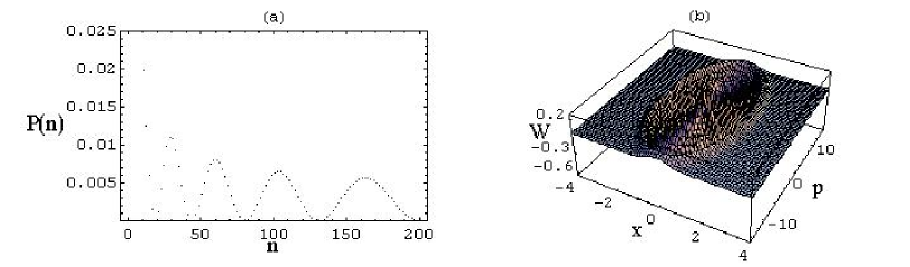
Figure 19: (a) Photon number distribution in the state $|\alpha,\varepsilon,m\rangle=|0,1.7,15\rangle$. A high value of the squeezing parameter $\varepsilon$ is chosen in order to magnify the oscillatory behavior. (b) Wigner function for the state $|0,1,15\rangle$.

As usual, we can compute the average number of photons $\langle n\rangle=m\cosh(2r)+\sinh^{2}r$, and the photon number variance $\langle\Delta n^{2}\rangle=\frac{1}{2}(m^{2}+m+1)\sinh^{2}(2r)$, which shows that the number uncertainty increases linearly with the initial value $m$ of the photon number. Nonclassical properties of the squeezed number states are witnessed by extended regions of negativity of the Wigner function, which are clearly visible in Fig. (19) (b), plotted for the state $|0,1,15\rangle$. More generally, phase space representations of displaced–squeezed number states and of their superpositions have been extensively investigated in Refs. [363, 364, 365]. Higher-order squeezing and nonclassical correlation properties, have been discussed in Ref. [359], and it has been shown that further nonclassical effects arise when displaced–squeezed number states are sent as inputs in a Kerr medium [366]. Finally, we wish to mention a recent successful experiment in the production of displaced Fock states of light [367]; their synthesis has been obtained by overlapping the pulsed optical single-photon number state with coherent states at a beam splitter with high reflectivity.

5.5 Displaced and squeezed Kerr states

Another interesting method to realize nonclassical states of light consists in associating displacement and squeezing with a third-order nonlinear, unitary Kerr evolution of the form $\exp\{-i\chi^{(3)}a^{{\dagger}2}a^{2}\}$. In Section 4, we showed that a typical Kerr state $|\psi\rangle_{K}$ is generated by applying the Kerr evolution operator to an initial coherent state: $|\psi\rangle_{K}=\exp\{-i\chi^{(3)}a^{{\dagger}2}a^{2}\}|\alpha\rangle$. On the other hand, in the same Section, we have seen that the Kerr interaction acts on the initial coherent state by modifying the phases of the number states, but leaves invariant the Poissonian statistics. To obtain modifications of the photon statistics, one can apply further interactions; for instance, the Kerr state $|\psi\rangle_{K}$ can be displaced, yielding the so called displaced Kerr state $|\psi\rangle_{DK}=D(\beta)|\psi\rangle_{K}$, which can be generated by the action of a nonlinear Mach-Zehnder interferometer. Considering this device, Kitagawa and Yamamoto [234] showed that the photon number fluctuations $\langle\Delta n^{2}\rangle$ in a displaced Kerr state are lowered to the value $\langle n\rangle^{1/3}$, as compared to the value $\langle n\rangle^{2/3}$ obtained in an amplitude-squeezed state. With some algebra the displaced Kerr states can be expressed in the Fock basis, $|\psi\rangle_{DK}=\sum_{n}c_{n}|n\rangle$, where the coefficients $c_{n}$ are given, e. g. in Ref. [368]. This expansion is handy when determining the analytic expressions of the photon number distribution and of the Husimi $Q$-function.

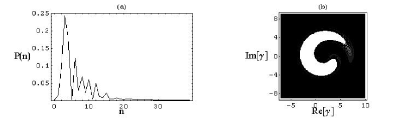
Figure 20: (a) Photon number distribution in the state $|\psi\rangle_{DK}=D(\beta)\exp\{-i\chi^{(3)}a^{{\dagger}2}a^{2}\}|\alpha\rangle$, plotted for $\alpha=3.5$, $\chi=0.25$, and $\beta=2$. (b) Contour plot of $Q(\gamma)\equiv\pi^{-1}|\langle\gamma|\psi\rangle_{DK}|^{2}$ for the same state.

In Fig. (20) (a) and (b) we show the photon number distribution $P(n)$ and the contour plot of $Q$, respectively; we see that, for the super-Poissonian case of Fig. (20) (a), the contour plot of the $Q$-function tends to become ring-shaped. It is worth mentioning that the photon statistics of a squeezed Kerr state $|\psi\rangle_{SK}=S(\varepsilon)|\psi\rangle_{K}$ is similar to that of the displaced Kerr states $|\psi\rangle_{DK}$. A detailed discussion of the statistical properties of the displaced and of the squeezed Kerr states can be found in Refs. [368, 369, 370, 371].
A further generalization of Kerr states is achieved by suitably combining squeezing, Kerr effect, and displacement. In Fig. (21) we represent a generalized version of a nonlinear Mach-Zehnder interferometer, obtained by adding to the standard device a quadrature-squeezed light generator.

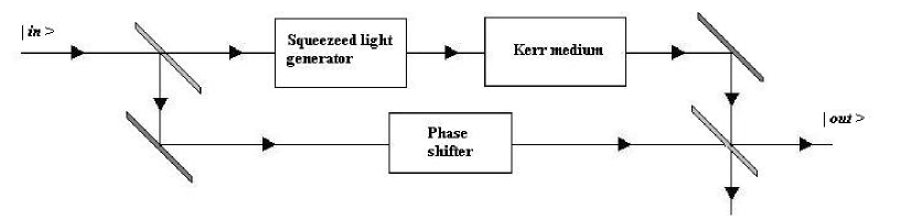
Figure 21: Schematic diagram of a nonlinear Mach-Zehnder interferometer for the generation of the displaced-Kerr-squeezed state $|\psi\rangle_{DKS}$.

This configuration has been proposed to produce the displaced-Kerr-squeezed state $|\psi\rangle_{DKS}=D(\beta)\exp\{-i\chi^{(3)}a^{{\dagger}2}a^{2}\}|\alpha,\varepsilon\rangle$, where $|\alpha,\varepsilon\rangle$ is a generic two-photon squeezed state. The displaced-Kerr-squeezed state $|\psi\rangle_{DKS}$ allows a further reduction in the photon number uncertainty down to the value $\langle n\rangle^{1/5}$ [369].

5.6 Intermediate (binomial) states of the radiation field

The examples discussed so far can naturally be generalized to conceive the engineering of states characterized by a specific (a priori assigned) probability distribution for the number of photons. In previous Sections we have studied systems associated with various statistical distributions, such as coherent states (with Poissonian distribution), thermal states (with Bose-Einstein distribution), squeezed states (with sub- or super-Poissonian distribution), and Fock states. In 1985, Stoler et al. [372] succeeded in introducing single-mode quantum states which interpolate between a coherent and a number state. They, in fact, introduced the binomial states, characterized by a binomial photon number distribution. The binomial states $|p,M\rangle_{B}$ can be written as a finite combination of the first $M+1$ number states:

$$|p,M\rangle_{B}\,=\,\sum_{n=0}^{M}\left[\left(\begin{array}[]{c}M\\ n\\ \end{array}\right)p^{n}(1-p)^{M-n}\right]^{1/2}|n\rangle\;,\;\quad 0<p<1\;,$$ (263)

where $\left(\begin{array}[]{c}M\\ n\\ \end{array}\right)$ is the usual binomial coefficient. The state $|p,M\rangle_{B}$ reduces to the coherent state in the limit $p\rightarrow 0$, $M\rightarrow\infty$, $pM=const$, while it realizes the number state $|M\rangle$ for $p\rightarrow 1$. The properties of the binomial states have been investigated in Refs. [372, 373, 374], and the methods for their generation have been proposed in Refs. [449, 372, 373, 375]. Binomial states appear to be strongly nonclassical. In fact, they exhibit intense second and fourth order squeezing (see definition (150)), whose maxima depend on $M$. Moreover, the statistics of these states is intrinsically sub-Poissonian, as the Mandel parameter $Q=-p$ [374], and their Wigner function exhibits a negative region, more and more pronounced for increasing $p$. Binomial states can be generated in a process of emission of $M$ photons, each one emitted with the same probability $p\;$; for instance, they can be produced from the vibrational relaxation of an excited molecule [372]. A simple generalization of the class of states (263), which is more flexible from the point of view of applications, can be obtained in the form [376]

$$|p,M,q\rangle_{GB}\,=$$

$$\sum_{n=0}^{M}\left[\left(\begin{array}[]{c}M\\ n\\ \end{array}\right)\frac{p}{1+Mq}\left(\frac{p+nq}{1+Mq}\right)^{n-1}\left(1-\frac{p+nq}{1+Mq}\right)^{M-n}\right]^{1/2}|n\rangle\;,$$ (266)

where the additional parameter $q$ satisfies the constraint $q\geq\max\left\{-\frac{p}{M}\,,-\frac{1-p}{M}\right\}$. The parameter $q$ can be tuned to control the nonclassical behavior and realize , for instance, a stronger sub-Poissonian statistics. Comparing Eqs. (263) and (266), it is evident that the emission events for different photons happen with different probabilities, at variance with the case of the standard binomial states. This implies that, in the process of generation of the generalized binomial state (266), the probability of photon emission cannot be the same for the different energy levels of an excited molecule [376].
A further typology of intermediate states is constituted by the negative binomial states [377, 378, 379, 380]. These states interpolate between the coherent and the thermal states, and are characterized by a negative binomial photon number distribution, which is, in a sense, the inverse of the binomial distribution, as it can be guessed by noting the inverted order of the factors in the binomial coefficient. In fact, the negative binomial quantum states are expressed in the form [381]

$$|\alpha,M\rangle_{NB}\,=\,(1-|\alpha|^{2})^{(M+1)/2}\sum_{n=M}^{\infty}\left(\begin{array}[]{c}n\\ M\\ \end{array}\right)^{1/2}\alpha^{n-M}|n\rangle\;,$$ (267)

where $\alpha=|\alpha|e^{i\phi}$, $0<|\alpha|<1$, and $M$ is a non-negative integer. A summary of the main properties of negative binomial states, and a comparison of these states with the binomial states and with other states of light, can be found in Refs. ([380, 382]). The states (267) can be prepared in optical multiphoton processes, in terms of $M$-photon absorptions from a thermal beam of photons, or by parametric amplification with suitable initial conditions [380]. It is also possible to conceive generation schemes of their superpositions [383, 384].
Finally, we wish to review the class of the reciprocal binomial states $|\Phi,M\rangle_{RB}$, introduced by Barnett and Pegg [385]. These states have been proposed as fiducial reference for the experimental reconstruction of the quantum optical phase probability distribution, in a scheme that mixes the signal field and the reference state $|\Phi,M\rangle_{RB}$ by means of a beam splitter. The reciprocal binomial state is defined as

$$|\phi,M\rangle_{RB}\,=\,\mathcal{N}^{-1}\sum_{n=0}^{M}\left(\begin{array}[]{c}M\\ n\\ \end{array}\right)^{-1/2}e^{in(\phi-\pi/2)}|n\rangle\;,$$ (268)

where $\mathcal{N}$ is a normalization factor. A scheme for the generation of the states (268), that can be used as well for the production of states (263) and (267), has been proposed in Ref. [386]; this proposal is related to the one by Vogel et al. [351]. The proposed experimental setup is shown in Fig. (22); it is composed by $M$ two-level (Rydberg) atoms, a Ramsey zone (R), a high-$Q$ cavity (C), and a field ionization detector (D).

Figure 22: Experimental setup for the generation of the reciprocal binomial states (268). The $M$ atoms are prepared by a microwave field $R$; they are injected in the cavity $C$; and, finally, they are counted in the ionization detector $D$.

The atoms are prepared, by a microwave field $R$ (Ramsey zone), in a superposition of the ground state $|g\rangle$ and of the excited state $|e\rangle\;$: $\;c_{g}^{(n)}|g\rangle_{(n)}+c_{e}^{(n)}|e\rangle_{(n)}\;$ (with $n$ labelling the $n$-th atom). The atoms are then injected one-by-one in the cavity. The on-resonant interaction of each atom with the cavity field is described by the Hamiltonian $H_{onres}=\omega_{1}(|e\rangle\langle g|a+|g\rangle\langle e|a^{{\dagger}})$, where we have dropped the index $n$. When all the $M$ atoms are detected in the ground state at the output of the cavity, the state of the cavity field becomes

$$\mathcal{N}^{-1}\sum_{n=0}^{M}\Lambda_{n}^{(M)}e^{-in\pi/2}|n\rangle\;,$$

with the coefficients $\Lambda_{n}^{(M)}$ given by the recurrence formula

$$\Lambda_{n}^{(M)}=(1-\delta_{n,0})\Lambda_{n-1}^{(M-1)}c_{e}^{(M)}\sin(\sqrt{n}\omega_{1}\tau_{M})+(1-\delta_{n,M})\Lambda_{n}^{(M-1)}c_{g}^{(M)}\cos(\sqrt{n}\omega_{1}\tau_{M})\;.$$

The procedure is concluded by sending an auxiliary atom in the cavity with an off-resonant interaction of the form $H_{offres}=\omega_{2}a^{{\dagger}}a(|e\rangle\langle e|-|g\rangle\langle g|)$. If the atom is prepared in the ground state, the off-resonant interaction produces, in the atomic states, a conditional phase shift $\phi$ controlled by the photon number in the cavity field. The reciprocal binomial state (268) is finally obtained by imposing a suitable form for the coefficients $\Lambda_{n}^{(M)}$, with $\phi=\omega_{2}T$ ($T$ being the duration of interaction) [386].
Besides the binomial states and their generalizations, several other classes of intermediate states of light have been constructed and investigated, such as logarithmic states [387] and multinomial states [388]. For a complete bibliography on this subject we refer to the review article [308].

5.7 Photon-added, photon-subtracted, and vortex states

Nonclassical states with very interesting properties are the so-called photon-added states $|\psi\,,k\rangle$, that are produced by repeated applications of the photon creation operator on an arbitrary quantum state $|\psi\rangle$:

$$|\psi\,,k\rangle\,=\,\mathcal{N}a^{{\dagger}k}|\psi\rangle\;,$$ (269)

where $\mathcal{N}$ is a normalization factor. Agarwal and Tara introduced a first type of states (269), the photon-added coherent states, by choosing for $|\psi\rangle$ the coherent state $|\alpha\rangle$ [389]:

$$|\alpha\,,k\rangle\,=\,\mathcal{N}(\alpha\,,k)a^{{\dagger}k}|\alpha\rangle\;,$$ (270)

where the normalization factor $\mathcal{N}(\alpha\,,k)=\langle\alpha|a^{k}a^{{\dagger}k}|\alpha\rangle^{-1/2}=[L_{k}(-|\alpha|^{2})k!]^{-1/2}$, with $L_{k}(x)$ the Laguerre polynomial of degree $k$. The photon-added coherent states (270) exhibit squeezing, and their photon number distribution is a shifted Poisson distribution of the form

$$P(n)\,=\,\mathcal{N}(\alpha\,,k)^{2}\frac{n!|\alpha|^{2(n-k)}}{[(n-k)!]^{2}}e^{-|\alpha|^{2}}\;.$$ (271)

In Fig. (23) (a) we have plotted the Mandel $Q$ parameter as a function of $|\alpha|$ for different choices of the number $k$ of added photons. We see that the Mandel parameter remains always below one, and decreases with increasing $k$, and the photon number distribution (271) describes a growingly stronger sub-Poissonian statistics [389]. A further signature of nonclassicality is provided by the fact that the Wigner function for these states

$$W\left(\xi=\frac{x+ip}{\sqrt{2}}\right)\,=\,\frac{2(-1)^{k}L_{k}(|2\xi-\alpha|^{2})}{\pi L_{k}(-|\alpha|^{2})}e^{-2|\xi-\alpha|^{2}}\;,$$ (272)

plotted in Fig. (23) (b), takes negative values due to the weights of the Laguerre polynomials.

Figure 23: (a) Plot of the $Q$ parameter of the photon-added coherent states (270) as a function of the coherent amplitude $|\alpha|$, for $k=5$ (full line), $k=15$ (dotted line), $k=25$ (dashed line), and $k=35$ (dot-dashed line). (b) Plot of the Wigner function $W(x,p)$ (272) for $k=15$ and $\alpha=2$.

Agarwal and Tara have proposed also a scheme for the production of photon-added states, based on nonlinear processes in a cavity. The interaction Hamiltonian describing the passage of two-level excited atoms ($k$-photon medium) through a cavity can be written in the form

$$H_{I}\,=\,\eta\sigma^{+}a^{k}+\eta^{*}\sigma^{-}a^{{\dagger}k}\;,$$ (273)

where $a$ is the cavity field mode, $\sigma^{+}=|e\rangle\langle g|$, $\sigma^{-}=|g\rangle\langle e|$, and the notation $\sigma^{\pm}$ refers to the fact that such atomic raising and lowering operators can be represented by Pauli matrices. If the initial state of the field-atom system is the factorized state $|\alpha\rangle|e\rangle$, then, for short (reduced, dimensionless) times $|\eta|t\ll 1$ the evolved state can be approximated by

$$|\psi(t)\rangle\,\approx\,|\alpha\rangle|e\rangle\,-\,i\eta^{*}ta^{{\dagger}k}|\alpha\rangle|g\rangle\;.$$ (274)

When the atom is detected in the ground state $|g\rangle$, then the photon-added coherent state will be generated in the process, apart from a normalization factor. Alternatively, the state $|\alpha\,,k\rangle$ may also be produced by methods based on state reduction and feedback [390].
Dodonov et al. [391] have studied the dynamics of the states $|\alpha\,,k\rangle$, when the field mode eigenfrequency $\omega$ is time-dependent, and the Hamiltonian ruling the time evolution is

$$H\,=\;\frac{1}{2}[P^{2}+\omega^{2}(t)Q^{2}]\;,\quad\quad\omega(t)\;=\;1+2\gamma\cos 2t\;,\;\;|\gamma|\ll 1\;.$$ (275)

The action of this Hamiltonian on photon-added coherent states produces new states that exhibit, under certain conditions, a larger degree of squeezing with respect to two-photon squeezed states, and a transition from the initial sub-Poissonian statistics to a super-Poissonian one.
Varying the choices of the reference state $|\psi\rangle$, many other types of photon added states can be obtained, such as the photon-added squeezed states [392], the even/odd photon-added states [393], and the photon-added thermal states [394]. Symmetrically to the photon-added states, one can as well define the class of the photon-subtracted states. The latter can be obtained by simply replacing the creation operator $a^{{\dagger}}$ with the annihilation operator $a$ in Eq. (269) [395, 396]. Proposals for the generation of photon-added and photon-subtracted states, based on conditional measurements, have been discussed in Refs. [395, 397].
A two-mode generalization of the degenerate photon-added states has been considered in Ref. [398]. Similar to these two-mode photon-added states are the two-mode vortex states of the radiation field [399], which are characterized by a wave function, in the two-dimensional configuration representation, of the form

$$\psi_{v}^{(m)}(x,y)\,=\,\frac{1}{\sqrt{m!\pi\sigma^{2m+2}}}(x-iy)^{m}e^{-\frac{1}{2\sigma^{2}}(x^{2}+y^{2})}\;.$$ (276)

The vortex structure of these states shows up in the intensity distribution function $|\psi_{v}^{(m)}(x,y)|^{2}$, plotted in Fig. (24).

Figure 24: Intensity distribution function for the vortex state (276) with $\sigma=\sqrt{2}$ and $m=5$.

In terms of the field mode operators $a$ and $b$, the vortex state can be recast in the form

$$|\psi_{v}^{(m)}\rangle\,=\,\mathcal{N}_{v}(a^{{\dagger}}-ib^{{\dagger}})^{m}e^{r(a^{{\dagger}2}-a^{2})}e^{r(b^{{\dagger}2}-b^{2})}|0,0\rangle\;,$$

$$\mathcal{N}_{v}\,=\,\frac{2^{-m/2}(1+\xi)^{m}}{\sqrt{m!}\sigma^{m}}\;,\quad\quad\xi\,=\,\frac{\sigma^{2}-1}{\sigma^{2}+1}\;,$$ (277)

where $\sigma=e^{2r}$. The nonclassical character of the state (277) emerges from the behavior of the second-order correlation functions. For different choices of $m$, we have plotted in Fig. (25) (a) and (b), respectively, the quantities $g^{(2)}_{aa,T}(0)=g^{(2)}_{aa}(0)-1$ and $g^{(2)}_{ab,T}(0)=g^{(2)}_{ab}(0)-1$, where $g^{(2)}_{aa}(0)$ is the auto-correlation of mode $a$, and $g^{(2)}_{ab}(0)$ is the cross-correlation between modes $a$ and $b$. The graphic shows that the field mode $a$ exhibits sub-Poissonian statistics, and that modes $a$ and $b$ are anticorrelated.

Figure 25: (a): plot of $g^{(2)}_{aa,T}(0)$. (b): plot of $g^{(2)}_{ab,T}(0)$. Both plots are dawn as functions of $\sigma$, and with $m=2$ (full line), $m=5$ (dotted line), and $m=10$ (dashed line).

A simple scheme to produce the vortex states, based on a three-level $\Lambda$ system interacting with two polarized fields on resonance, has been proposed in Ref. [399].

5.8 Higher-power coherent and squeezed states

Among the many nonclassical generalizations of Glauber’s coherent states, the even and odd coherent states are of particular relevance. They are defined as two particular classes of eigenstates of $a^{2}$, respectively with even and odd number of photons. All the remaining eigenstates can then be obtained as arbitrary linear combinations of even and odd coherent states. These states were introduced by Dodonov, Malkin, and Man’ko [315], and can be written in the following form:

$$|\alpha\rangle_{even} \,=\, (\cosh|\alpha|^{2})^{-1/2}\sum_{n=0}^{\infty}\frac{\alpha^{2n}}{\sqrt{(2n)!}}|2n\rangle\;,$$ (278)

$$|\alpha\rangle_{odd} \,=\, (\sinh|\alpha|^{2})^{-1/2}\sum_{n=0}^{\infty}\frac{\alpha^{2n+1}}{\sqrt{(2n+1)!}}|2n+1\rangle\;.$$ (279)

These two classes of coherent states have been later generalized by introducing the $j$-th order coherent states, defined as the eigenstates of $a^{j}$ [400, 401, 402]:

$$a^{j}|\alpha;j,k\rangle\,=\,\alpha^{j}|\alpha;j,k\rangle\;,$$ (280)

where, as will be clarified, the notation $j,k$ indicates that the states $|\alpha;j,k\rangle$ can be written as superpositions of the Fock states $\{|jn+k\rangle\}$, with the additional integer parameter $k$ restricted to be $0\leq k\leq j-1$. We recall that a subclass of these states can be generated at suitable times by a Kerr interaction (see Section 4), and that the even and odd coherent states are a particular realization of the Barut-Girardello coherent states, already introduced in this Section.
The solution of Eq. (280) is given by the infinite superposition

$$|\alpha;j,k\rangle\,=\,S^{-1/2}(j,k,|\alpha|^{2})\sum_{n=0}^{\infty}\frac{\alpha^{jn+k}}{\sqrt{(jn+k)!}}|jn+k\rangle\;,$$ (281)

where

$$S(j,k,z)\,=\,\sum_{n=0}^{\infty}\frac{z^{jn+k}}{(jn+k)!}\;.$$ (282)

To any fixed eigenvalue $\alpha$ in the equation (280) are associated $j$ solutions for the $j$-th order coherent states. It can be seen that the standard coherent states coincide with the unique solution $|\alpha;1,0\rangle$ for $j=1$ and $k=0$. Moreover, the two solutions with $j=2\,,k=0$ and $j=2\,,k=1$, $|\alpha;2,0\rangle$ and $|\alpha;2,1\rangle$, coincide, respectively, with the even and odd coherent states. Nieto and Truax [402] have computed the wave function solution of the equation (280). It can be expressed in terms of the following generalized generating functions for the Hermite polynomials

$$G(j,k,x,z)\,=\,\sum_{n=0}^{\infty}\frac{z^{jn+k}H_{jn+k}(x)}{(jn+k)!}\;,$$ (283)

and, consequently, cast in the form [402]

$$\langle x|\alpha\,,jk\rangle\,=\,\frac{e^{-\frac{1}{2}x^{2}}G(j,k,x,\alpha/\sqrt{2})}{\pi^{1/4}S^{1/2}(j,k,|\alpha|^{2})}\;.$$ (284)

Among the main properties of the states $|\alpha;j,k\rangle$, the following relations of orthogonality can be easily verified

$$\langle\alpha;j,k|\alpha;j,k^{\prime}\rangle\,=0\,\;,\quad\quad k\neq k^{\prime}\,=\,0,1,...,j-1\;,$$

$$\langle\alpha;j,k|\alpha;j^{\prime},k^{\prime}\rangle\,=\,\delta_{jn+k\,,\,j^{\prime}n^{\prime}+k^{\prime}}\;,\quad\quad j,j^{\prime}\geq 3\;,$$

$$k\,=\,0,1,...,j-1\;,\quad k^{\prime}\,=\,0,1,...,j^{\prime}-1\;,\quad n,n^{\prime}\,=\,0,1,...\;,$$ (285)

while the relation

$$\frac{1}{\pi}\int d^{2}\alpha\sum_{k=0}^{j-1}|\alpha;j,k\rangle\,\langle\alpha;j,k|=1$$ (286)

gives a complete representation with respect to $\alpha$. Moreover, for $\alpha\neq\alpha^{\prime}$ the states $|\alpha;j,k\rangle$ and $|\alpha^{\prime};j,k\rangle$ are not orthogonal; therefore, the generalized coherent states $|\alpha;j,k\rangle$ form an overcomplete set with respect to $\alpha$. In addition, any orthonormalized eigenstate of $a^{j}$ can be recast in the form of a superposition of $j$ coherent states with different phases:

$$|\alpha;j,k\rangle\,=\,\frac{e^{\frac{1}{2}|\alpha|^{2}}}{jS^{1/2}(j,k,|\alpha|^{2})}\sum_{l=0}^{j-1}e^{i\frac{2\pi}{j}k(j-l)}|\alpha e^{i\frac{2\pi}{j}l}\rangle\;.$$ (287)

The states $|\alpha;j,k\rangle$ do not enjoy second-order squeezing, because they are not minimum uncertainty states of the canonically conjugated quadrature operators. On the other hand, all the generalized coherent states $|\alpha;j,k\rangle$ exhibit antibunching effects, and satisfy the definition of $N$-th order squeezing in the sense of Zhang et al. [403]. Given the operators

$$Z_{1}(N)\,=\,\frac{1}{2}(a^{{\dagger}N}+a^{N})\;,\quad\quad Z_{2}(N)\,=\,\frac{i}{2}(a^{{\dagger}N}-a^{N})\;,$$ (288)

these authors, at variance with the more common criterion (150), define the $N$-th order squeezed states as those which satisfy the relation

$$\langle\Delta Z_{i}^{2}(N)\rangle\,<\,\frac{1}{4}\langle[a^{N},a^{{\dagger}N}]\rangle\;,\quad\quad i=1,2\;.$$ (289)

J. Sun, J. Wang, and C. Wang have proved that the generalized coherent states $|\alpha;j,k\rangle$ exhibit $N$-th order squeezing, in the sense of Eq. (289), if $N=(m+\frac{1}{2})j$, $m=0,1,...$, and $j$ even. On the contrary, no state $|\alpha;j,k\rangle$ with $j$ odd possesses higher-order squeezing [401]. The same authors have shown that, both for odd and for even degree $j$, all the states $|\alpha;j,k\rangle$ are minimum uncertainty states for the pair of operators $Z_{1}(N)$ and $Z_{2}(N)$, with $N=mj$ ($m=1,2,...$). Finally, we mention that in Ref. [404], the one-mode $j$-th order coherent states have been generalized to the multimode instance through the following definition of the multimode higher order coherent states $|\Psi\rangle_{kl...m}$:

$$a^{k}b^{l}...c^{m}|\Psi\rangle_{kl...m}\,=\,\alpha^{k}\beta^{l}...\gamma^{m}|\Psi\rangle_{kl...m}\;.$$ (290)

Analogous techniques can be exploited to define the $j$-th order squeezed states (which must not be confused with the concept of higher order squeezing of a state), as the solutions of the eigenvalue equation [402]

$$\left[\frac{1}{2}(1+\lambda)a^{j}+\frac{1}{2}(1-\lambda)a^{{\dagger}j}\right]|\beta,\lambda;j,k\rangle\,=\,\beta^{j}|\beta,\lambda,jk\rangle\;.$$ (291)

When $\lambda\rightarrow 1$, the $j$-th order squeezed states reduce to $j$-th order coherent states, and they reduce to the standard Glauber coherent states for $j=\lambda=1$. However, they never reduce to the standard two-photon squeezed states. The second order ($j=2$) squeezed states present interesting features [405]. For instance, the variances of the amplitude-squared operators $\langle\Delta Z_{i}^{2}\rangle$, and the second order correlation function at the initial time $g^{(2)}(0)$ for a second order squeezed state are functions of the mean photon number $\langle a^{{\dagger}}a\rangle$, and take the forms:

$$\langle\Delta Z_{1}^{2}\rangle\,=\,\lambda\left(\langle a^{{\dagger}}a\rangle+\frac{1}{2}\right)\;,\quad\quad\langle\Delta Z_{2}^{2}\rangle\,=\,\frac{1}{\lambda}\left(\langle a^{{\dagger}}a\rangle+\frac{1}{2}\right)\;,$$ (292)

$$g^{(2)}(0)\,=\,\frac{1}{\langle a^{{\dagger}}a\rangle^{2}}\left\{\frac{(\lambda-1)^{2}}{\lambda}\left(\langle a^{{\dagger}}a\rangle+\frac{1}{2}\right)+Re[\beta^{2}]^{2}+\frac{1}{\lambda^{2}}Im[\beta^{2}]^{2}\right\}\;.$$ (293)

From the two relations in Eq. (292), it follows that the parameter $\lambda$ is a squeezing factor, and can be expressed as the square root of the ratio $\langle\Delta Z_{1}^{2}\rangle/\langle\Delta Z_{2}^{2}\rangle$.
Finally, in Ref. [406] it has been shown that the orthonormal eigenstates of an arbitrary power $b^{j}$ of the linear combination $b=\mu a+\nu a^{{\dagger}}$ (with $\mu$, $\nu$ satisfying the Bogoliubov condition of canonicity) can be constructed by applying the squeezing operator $S(\varepsilon)$ to the $j$-th order coherent states (281)

$$|\beta;j,k\rangle_{g}\,=\,S(\varepsilon)|\beta;j,k\rangle\,=\,\{\langle\beta|P_{k}^{j}|\beta\rangle\}^{-1/2}S(\varepsilon)P_{k}^{j}|\beta\rangle\;,$$

$$k=0,1,...,j-1\,,$$ (294)

where $P_{k}^{j}$ is a generalized projection operator defined by

$$P_{k}^{j}\,=\,\sum_{n=0}^{\infty}|jn+k\rangle\langle jn+k|\;,k=0,1,...,j-1\;.$$ (295)

For the particular choice $j=2$, the operators $P_{k}^{j}$ $(k=0,1)$ and $S(\varepsilon)$ commute, and the states (294) become the so-called even and odd two-photon coherent states, given by

$$|\beta;2,0\rangle_{g}\,=\,(\cosh|\beta|^{2})^{-1/2}e^{\frac{|\beta|^{2}}{2}}P_{0}^{2}|\beta\rangle_{g}\;,$$

$$|\beta;2,1\rangle_{g}\,=\,(\sinh|\beta|^{2})^{-1/2}e^{\frac{|\beta|^{2}}{2}}P_{1}^{2}|\beta\rangle_{g}\;,$$ (296)

where $|\beta\rangle_{g}$ is a the standard Yuen two-photon coherent state. In Ref. [406], it is shown that both even and odd two-photon coherent states exhibit squeezing for suitable choices of the parameters, and that a strong antibunching effect is exhibited by the odd states, while this antibunching effect, although still present, is sensibly weaker in the case of even states.

5.9 Cotangent and tangent states of the electromagnetic field

The class of cotangent and tangent states of the electromagnetic field have been introduced and discussed in Refs. [407]. These states can be generated in a high-$Q$ micromaser cavity by the evolution of the harmonic oscillator (cavity mode) coupled to a “quantum current” consisting of a beam of two-level atoms, whose initial state is given by a superposition of the upper and lower atomic states. The effective interaction is described, as usual, by a Jaynes-Cummings Hamiltonian, with exact resonance between the field frequency and the atomic transition frequency. Moreover, it is assumed that only one atom at a time is present inside the resonator, and that the state of the atom is not measured as it leaves the cavity. However, the passage of each atom induces a nonselective measurement [408], described by a partial trace operation on the density matrix of the total system over the atom variables. Cotangent and tangent states are generated during the time evolution as finite superpositions of the form:

$$|\Psi\rangle_{c,t}\,=\,\sum_{n=N}^{M}s_{n}|n\rangle\;.$$ (297)

Here $N,\,M$ are the number indices associated to “trapping states”, and determined by the conditions

$$\kappa\sqrt{N}\tau\,=\,q\,\pi\qquad,\qquad\kappa\sqrt{M+1}\tau=\,p\,\pi\;,$$ (298)

where, $q,\,p$ are integer numbers, $\kappa$ is the Jaynes-Cummings cavity-atom coupling, and $\tau$ is the interaction time between a single atom and the cavity. The coefficients $s_{n}$ in Eq. (297) are given by

$$s_{n}\,=\,\mathcal{N}_{c}(-i)^{n}(\alpha/\beta)^{n}\prod_{j=1}^{n}\cot(\kappa\sqrt{j}\tau/2)\;,$$ (299)

for the choice of $q$ even and $p$ odd in Eq. (298) (cotangent states), and by

$$s_{n}\,=\,\mathcal{N}_{t}(i)^{n}(\alpha/\beta)^{n}\prod_{j=1}^{n}\tan(\kappa\sqrt{j}\tau/2)\;,$$ (300)

for the choice of $q$ odd and $p$ even in Eq. (298) (tangent states), with $\mathcal{N}_{c},\,\mathcal{N}_{t}$ normalization constants. Cotangent and tangent states, under suitable conditions, can exhibit sub-Poissonian photon statistics or, alternatively, they resemble macroscopic superpositions [407]; these nonclassical properties are in principle remarkably robust under the effects of cavity damping [409]. Finally, in Ref. [410] it has been shown that these states, under a wide range of conditions, are highly squeezed, and that the phase distribution can exhibit oscillations resulting from the formation of states that are again reminiscent of macroscopic superpositions.

5.10 Quantum state engineering

In the previous Subsections we have reviewed several schemes for the generation of nonclassical multiphoton states of light beyond the standard two-photon squeezed states. However, all these schemes are tied to particular contexts and specific descriptions. It would be instead desirable to implement a general procedure which allows, at least in principle, to engineer nonclassical multiphoton states of generic form. Several attempts in this direction have resulted in two main approaches. One approach is based on the time evolution generated by a generic, controlling Hamiltonian which drives an initial state to the final target state (pure state, unitary evolution). Another approach is realized in two steps: first, the quantum system of interest is correlated (entangled) with another auxiliary system; next, a measurement is performed on the auxiliary system, reducing the state of the system of interest to the desired target state. In the following we briefly review some of the most relevant methods, thus providing a compact introduction to quantum state engineering in the framework of multiphoton quantum optics.

a)    Clearly, the simplest theoretical and experimental ways to produce nonclassical states of light is based on the processes of amplification in $\chi^{(2)}$ and $\chi^{(3)}$ media. The signal and the idler beams of the (nonclassical) squeezed light, generated in nondegenerate parametric down conversion, exhibit strong space-time correlations. A destructive measurement on the idler output may lead to the generation and$/$or manipulation of nonclassical states of light at the signal output. Many papers have been devoted to various applications of this strategy [411, 412, 413, 414, 415, 416, 417, 418, 419]; in the following we review some of the most relevant results. A feedback measurement scheme has been proposed by Yuen to produce near-photon-number-eigenstate fields [411]. A quantum nondemolition measurement of the number of photons can be performed to generate a number-phase squeezed state [236]. In Ref. [390] the outcome of a homodyne measurement of the idler wave is used to manipulate the signal wave by means of feed forward, linear attenuators, amplifiers, or phase modulators. A detailed analysis of the effect on the signal output of a measurement on the idler output, described by a POVM (positive operator-valued measure or generalized projection) [408], has been performed by Watanabe and Yamamoto [413]. In particular, these authors have studied the application of three different state-reduction measurements (expressed in terms of projection operators) leading to different output signal fields. If the idler photon number is measured by a photon counter, the signal wave is reduced to a number-phase squeezed state; if the idler single-quadrature amplitude is measured by homodyne detection, the signal wave is reduced to a quadrature-amplitude squeezed state; if the idler two-quadrature amplitudes are measured by heterodyne detection, the signal wave is reduced to a coherent state [413]. In Ref. [414], Ueda et al. have developed a general theory of continuous state reduction, by substituting the POVM with suitable superoperators. More recently, arbitrary generalized measurements have been considered in Ref. [416]. It has been shown [418] that the action on a twin beam of an avalanche photodetector, described by a specific POVM, may lead to a highly nonclassical reduced state, characterized by a Wigner function with negative regions. The possibility of generating nonclassical states with sub-Poissonian photon-number statistics has been investigated as well. For instance, the experimental generation of sub-Poissonian light has been obtained by using a negative feedback sent to the pump from the idler wave of a twin beam [412]. In Ref. [419], a particular homodyne detection, with randomized phases and in a defined range of the quadrature eigenvalues, has been proposed to reduce an initial twin beam to a sub-Poissonian field.
We remark that these methods have recently led to the successful experimental generation of several nonclassical states of light [420, 421, 422, 423, 424, 425]. All these eperiments combine parametric amplification and state-reduction techniques.

As relevant examples we describe in some detail the beautiful and encouraging experimental observation of single-photon-added states reported by Zavatta, Viciani, and Bellini [420], and of single-photon-subtracted states reported by Wenger, Tualle-Brouri, and Grangier [421]. The experimental setup used by Zavatta et al. is schematically depicted in Fig. (26); the production of the state $|\alpha,\,1\rangle=(1+|\alpha|^{2})^{-1/2}a^{{\dagger}}|\alpha\rangle$, with $|\alpha\rangle$ denoting a coherent state, is obtained exploiting the process of nondegenerate parametric amplification of the initial state $|\alpha\rangle_{s}|0\rangle_{i}$, where the subscripts $s$ and $i$ denote the signal and the idler beam, respectively. By keeping the parametric gain $g$ sufficiently low, the output state $|\psi_{out}\rangle$ can be written in the form

$$|\psi_{out}\rangle\,\propto\,(1+ga_{s}^{{\dagger}}a_{i}^{{\dagger}})|\alpha\rangle_{s}|0\rangle_{i}\,=\,|\alpha\rangle_{s}|0\rangle_{i}+ga_{s}^{{\dagger}}|\alpha\rangle_{s}|1\rangle_{i}\;.$$ (301)

From Eq. (301) it is clear that if the idler field is detected in the state $|1\rangle_{i}$, then the signal output field is just the state $|\alpha,\,1\rangle$, that is the single-photon-added state for $\alpha\neq 0$, and the one-photon number state for $\alpha=0$.

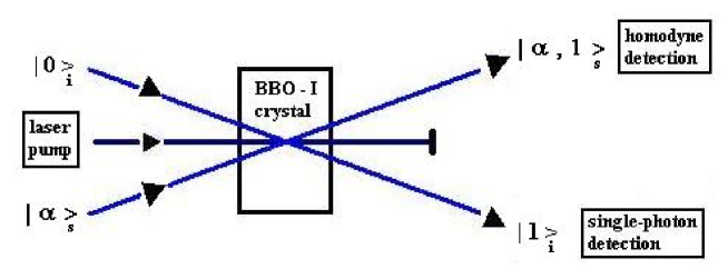
Figure 26: Experimental scheme for the preparation of a single-photon-added coherent state. It is based on a parametric down conversion process in a type-I beta-barium borate (BBO) crystal; initially, the signal field is in a coherent state (seed field), while the idler field is in the vacuum state. The generation of the one-photon-added coherent state is conditioned to the detection of one photon in the output idler mode. The output signal state is then characterized and reconstructed by standard quantum tomographical techniques.

The output single-photon-added coherent state is then reconstructed by exploiting techniques of quantum tomography (homodyne measurements). By gradually increasing the amplitude $\alpha$, a spectacular transition occurs from the quantum one-photon number state $|1\rangle_{s}$ at $\alpha=0$ to a classical (high intensity) coherent state at sufficiently high values of $|\alpha|$. The single-photon-added coherent state describes the continuous and smooth intermediate regimes between these two extremes.
The experimental realization of one-photon-subtracted states has been recently reported by Wenger et al. [421]. A simplified description of the experimental setup is depicted in Fig. (27).

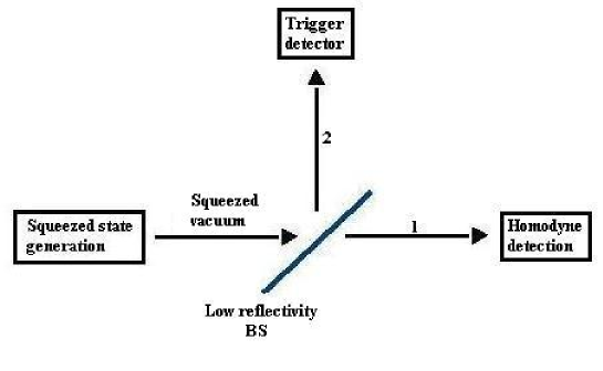
Figure 27: Experimental scheme for the preparation of a one-photon-subtracted state. The twin beam, obtained in the process of degenerate parametric amplification in a crystal of potassium niobate (KNbO₃) is sent to a low reflectivity beam splitter. The reflected wave is detected by a silicon avalanche photodiode, while the transmitted wave is sent to a homodyne detection. This scheme provides a degaussification protocol that maps pulses of squeezed light onto non-Gaussian states.

A single-mode squeezed vacuum $|sv\rangle$, with the squeezing parameter fixed at $r=0.43$, is sent to a beam splitter with low reflectivity $R\ll 1$; the statistics of the transmitted signal wave is reconstructed by using a balanced homodyne detector (with detection efficiency $\eta=0.75$), while the small reflected fraction of the squeezed vacuum beam is detected by an avalanche photodiode. The postselection then provides non-Gaussian (nonclassical) statistics. The reconstruction of the state is obtained numerically by considering the expansion of the squeezed vacuum state in the Fock basis $\{|n\rangle\}$ up to $n=10$. However, for the sake of simplicity and to illustrate the procedure, the authors report the calculations by truncating at $n=4$:

$$|sv\rangle=\gamma_{0}|0\rangle+\gamma_{1}|2\rangle+\gamma_{2}|4\rangle\;,$$ (302)

with $\gamma_{0}=0.96,\,\gamma_{1}=0.27,\,\gamma_{2}=0.10$. The passage through the beam splitter yields the output state $|sv\rangle_{BS}$:

$$|sv\rangle_{BS} = (\gamma_{0}|0\rangle_{1}+T^{2}\gamma_{1}|2\rangle_{1}+T^{4}\gamma_{2}|4\rangle_{1})|0\rangle_{2}$$ (303)

$$+ (\sqrt{2}RT\gamma_{1}|1\rangle_{1}+2RT^{3}\gamma_{2}|3\rangle_{1})|1\rangle_{2}+\mathcal{O}(2)\;,$$

where $T$ and $R$ denote the transmittance and the reflectivity of the beam splitter, respectively; $|\cdot\rangle_{1}$ and $|\cdot\rangle_{2}$ denote, respectively, the states of the transmitted and reflected modes; and $\mathcal{O}(2)$ represents higher-order terms containing Fock states $|m\rangle_{2}$ with $m>1$. Conditional detection of the state $|1\rangle_{2}$ leads to the generation of the non-Gaussian state:

$$|sv\rangle_{cond}\propto\gamma_{1}|1\rangle_{1}+\sqrt{2}\gamma_{2}T^{2}|3\rangle_{1}\;.$$ (304)

Having started from the truncated superposition that includes $|0\rangle$, $|2\rangle$, and $|4\rangle$, the above superposition is clearly the associated one-photon-subtracted state.
Using a postselection scheme similar to that of Ref. [420], Resch et al. have experimentally engineered a superposition of the form $\alpha|0\rangle+\beta|1\rangle$ [422]. In Refs. [423, 424], conditional parametric amplification has been used to produce high-fidelity quantum clones of a single-photon input state. Finally, the conditional preparation of a bright sub-Poissonian beam (from a twin beam) has been reported in Ref. [425], and theoretically analyzed in Ref. [426].

b)    In Ref. [351] Vogel, Akulin and Schleich have developed the second approach, and provided a recipe to construct, in principle, a generic quantum state of the radiation field. Their scheme, already illustrated in Subsection 5.6, Fig. (22), for the production of the reciprocal binomial states, is based on the interaction of $N$ two-level atoms with a resonant mode in a cavity. This interaction can be typically described by the Jaynes-Cummings Hamiltonian [23]. Initially, the cavity field is prepared in the vacuum state. One atom at a time is injected in the cavity in a superposition of the excited state $|e\rangle$ and of the ground state $|g\rangle$: $|e\rangle+i\epsilon_{k}|g\rangle$, where $\epsilon_{k}$ denotes a complex controlling parameter associated to the $k$-th atom. Let us suppose that $k-1$ atoms have been injected in the cavity without performing any measurement; then, the cavity field will evolve towards a state of the general form $|\psi^{(k-1)}\rangle=\sum_{n=0}^{k-1}\psi_{n}^{(k-1)}|n\rangle$, where the coefficients $\psi_{n}^{(k-1)}$ must be suitably determined recursively, as we will see later. Let us suppose now that a measurement is performed on the $k$-th atom at the output of the cavity. If this atom is detected in the excited state, the whole procedure must be repeated. If instead the $k$-th atom is detected in its ground state, it can be easily proved that the new state of the cavity field is

$$|\psi^{(k)}\rangle\,=\,\sum_{n=0}^{k}\psi_{n}^{(k)}|n\rangle\;,$$ (305)

$$\psi_{n}^{(k)}\,=\,\sin(\lambda\tau_{k}\sqrt{n})\psi_{n-1}^{(k-1)}-\epsilon_{k}\cos(\lambda\tau_{k}\sqrt{n})\psi_{n}^{(k-1)}\;,$$ (306)

where $\lambda$ denotes the atom-field coupling constant, and $\tau_{k}$ denotes the interaction time. Therefore, the passage of each atom increases by one unit the number of Fock states appearing in the finite superposition. If the target state to be engineered is of the generic form $|\psi_{tar}\rangle=\sum_{n=0}^{N}c_{n}|n\rangle$, where the $N+1$ coefficients $c_{n}$ have been fixed a priori, one must send in the cavity $N$ two-level atoms. Moreover, it can be shown that the initial internal states of the $N$ atoms can be prepared in such a way that the controlling parameters $\epsilon_{1},\ldots,\epsilon_{N}$ assure the identification $\psi_{n}^{(N)}=c_{n}$, $\forall\;n$. This completes the procedure.

c)    A scheme similar to that described above, exploiting Jaynes-Cummings models in high-$Q$ cavities, has been proposed for the generation of superpositions states, and in particular of macroscopic quantum superpositions [427, 428, 429, 430]. A nice proposal is due to Meystre, Slosser and Wilkens [427]. These authors consider, at very low temperature, a micromaser cavity pumped by a stream of polarized two-level atoms, and show that macroscopic superpositions are generated in the cavity. Moreover, they show that the onset of these superpositions can be interpreted in terms of a first order phase transition; at variance with the usual bistable systems involving incoherent mixture of the states localized at the two minima of an effective potential, this transition is characterized by coherent superpositions of such states.
In Refs. [429, 430] it has been introduced a method for the generation of mesoscopic (macroscopic) superpositions, that is based on a two-photon resonant Jaynes-Cummings model, in which a cascade of two atomic transitions of the kind $|e\rangle\rightarrow|i\rangle\rightarrow|g\rangle$ is resonant with twice the field frequency $\omega$: $\omega_{eg}=2\omega$. Here and in the following $\omega_{eg}$, $\omega_{ig}$, will denote the transition frequencies from the excited state $|e\rangle$ and the intermediate state $|i\rangle$ of an atom to its ground state $|g\rangle$, $\omega_{ei}$ will denote the transition frequency from the excited state $|e\rangle$ to the intermediate state $|i\rangle$, and $\Omega_{eg}$, $\Omega_{ig}$, $\Omega_{ei}$ will denote the Rabi frequencies associated to the same pairs of states. The intermediate transition frequences $\omega_{ig}$ and $\omega_{ei}$ are assumed strongly detuned from $\omega$ by $\Delta/2=\omega-\omega_{ei}=\omega_{ig}-\omega$. The dynamic evolution in the two-photon resonant Jaynes-Cummings model can be obtained in complete analogy to the ordinary one-photon model, by noting that the intermediate state $|i\rangle$ can be eliminated. In fact, by introducing the effective Rabi frequency [431] $\Omega_{n}=[(\Omega_{ei}^{2}+2\Omega_{ig}^{2})+n(\Omega_{ei}^{2}+\Omega_{ig}^{2})]/\Delta$, corresponding to an $n$-photon Fock state between $|e\rangle$ and $|g\rangle$, the state $|i\rangle$ remains unpopulated during the atom-fied interaction time $t$ if the condition $\Omega_{n}^{2}\,t/|\Delta|\ll\pi$ is satisfied [432]. Let us consider the case in which a single atom is initially in the excited state $|e\rangle$, and the cavity field is in an arbitrary state; the whole atom-field state is then of the factorized form $|\Psi(0)\rangle\equiv|e\rangle|\Psi_{c}(0)\rangle=|e\rangle\sum_{n=0}^{\infty}c_{0}(n)|n\rangle$. After a time $t$, in which the atom-field state evolves from $|\Psi(0)\rangle$ to $|\Psi(t)\rangle$, we can perform a conditional measurement on the atom, obtaining as output the excited state with a probability $P_{e}=|\langle e|\Psi(t)\rangle|^{2}$. If state $|e\rangle$ is effectively observed, the coefficients $c_{1}(n)$ of the new state of the field in the cavity, $|\Psi_{c}(t)\rangle=\sum_{n=0}^{\infty}c_{1}(n)|n\rangle$, can be computed in terms of the initial coefficients $\{c_{0}(n)\}$, the effective Rabi frequencies, and the probability $P_{e}$, and they read $c_{1}(n)=(P_{e})^{-1/2}c_{0}(n)\cos(\Omega_{n+2}t/2)$. At this stage of the procedure any quantum state can be, in principle, obtained. However, if an initial coherent state $|\alpha\rangle$ is chosen (i.e. if the initial coefficients $c_{0}(n)$ are the coefficients of the coherent superposition), the state $|\Psi_{c}(t)\rangle$ describes a mesoscopic superposition of coherent states. The method can be easily generalized [430] to conditional excitation measurements on $M$ atoms, leading to more complex superpositions, and to a better control on the statistics of the states.
It is to be remarked that decoherence effects make very difficult to implement the methods to create mesoscopic or macroscopic superpositions of states of the radiation field. However, exploiting high-$Q$ cavities, in 1996, Brune et al. have succeeded in obtaining an experimental realization of a mesoscopic superposition of an ”atom $+$ measuring apparatus” (atom $+$ cavity field) of the form $|\Psi_{cat}\rangle=2^{-1/2}(|e,\alpha e^{i\phi}\rangle+|g,\alpha e^{-i\phi}\rangle)$, and in observing its progressive decoherence [433]. Moreover, in 1997, Raimond et al. have prepared a Schödinger cat made of few photons, and studied the dynamics of its decoherence [434]. Both these experiments constitute a cornerstone in the investigation of the quantum/classical boundary by quantum optical methods. For a review on this subject see Ref. [435].

d)    An interesting proposal to control quantum states of a cavity field by a pure unitary evolution is based on a two-channel approach (both classical and quantum controlling radiation fields) [436]. A two-level atom in the cavity interacts with an external classical field $E_{ext}(t)$, and is coupled as well with the quantum cavity field $a$, with coupling constant $g(t)$. In resonance conditions, the controlling interaction Hamiltonian is given by [436]

$$H_{I}(t)\,=\,[E_{ext}(t)+\lambda(t)a]\sigma^{+}\,+\,H.c.\;,$$ (307)

where $\sigma^{\pm}$ represent the standard Pauli matrix notation for the atomic transitions. The controlling interaction can force the initial state $|\Psi(0)\rangle=|0,g\rangle$ of the system, i.e. the product of the vacuum cavity field state and of the atomic ground state, to evolve during a time $\tilde{t}$ towards the general (again factorized) final form $|\Psi(\tilde{t})\rangle=\sum_{n=0}^{M}c_{n}|n,g\rangle$. The procedure can be engineered as follows. The time interval $[0,\tilde{t}]$ is divided in the subintervals of equal lengths, $0<\tau<2\tau\cdots<j\tau<(j+1)\tau\cdots<(2M-1)\tau<\tilde{t}\,,\;$ $\tau=\tilde{t}/2M$. Further, the classical and the quantum channel are led to act alternatively on the time subintervals, by assuming for the functions $E_{ext}(t)$ and $\lambda(t)$ the following step-periodic time modulation:

$$\left\{\begin{array}[]{c}E_{ext}(t)=E_{j}\\ \lambda(t)=0\end{array}\right.\;,\quad\quad for\quad 2(j-1)\tau\,<\,t\,<\,(2j-1)\tau\;$$ (310)

$$\left\{\begin{array}[]{c}E_{ext}(t)=0\\ \lambda(t)\,=\,\lambda_{j}\end{array}\right.\;,\quad\quad for\quad(2j-1)\tau\,<\,t\,<\,2j\tau\;,$$ (313)

where $E_{j}$ and $\lambda_{j}$ $(1\leq j\leq M)$ are complex constants. The time evolution operator of the system is, thus, given by a product of evolution operators associated with each time interval, in the form

$$U(\tilde{t})=Q_{M}C_{M}Q_{M-1}C_{M-1}\cdots Q_{2}C_{2}Q_{1}C_{1}\,,$$ (314)

where $Q_{j}$ and $C_{j}$ represent, respectively, the quantum and the classical evolutions in the $j$-th interval, and can be expressed in the form of $2\times 2$ matrices [436]. The controlling values $\{E_{j}\}$ and $\{\lambda_{j}\}$ of the external classical field and of the quantum coupling can be finally determined by solving the equation of motion of the time reversed evolution

$$|0,g\rangle\,=\,U(-\tilde{t})|\Psi(\tilde{t})\rangle\,=\,C_{1}^{{\dagger}}Q_{1}^{{\dagger}}\cdots C_{M}^{{\dagger}}Q_{M}^{{\dagger}}|\Psi(\tilde{t})\rangle\;,$$ (315)

which, by connecting the desired final state to the given initial state, completes the procedure. The possible realization of this model in a cavity through a two-channel Raman interaction has been discussed as well in Ref. [436]. A further scheme for the engineering of a general field state in a cavity, which, at variance with the previous case, is not empty but prepared in a coherent state, has been considered in Ref. [437].

e)    Arbitrary multiphoton states of a single-mode electromagnetic field can be produced as well by exploiting discrete superpositions of coherent states along a straight line or on a circle in phase space [438, 439]. To this aim, let us consider, for instance, the discrete superposition of $n+1$ coherent states symmetrically positioned on a circle with radius $r$ [438]:

$$|n,r\rangle\,=\,\mathcal{N}(r)\frac{\sqrt{n!}e^{r^{2}/2}}{(n+1)r^{n}}\sum_{k=0}^{n}e^{\frac{2\pi i}{n+1}k}|re^{\frac{2\pi i}{n+1}k}\rangle\;,$$ (316)

where the coherent amplitude $\alpha_{k}$ of the $k$th coherent state entering the superposition, reads $\alpha_{k}=r\exp\{(2ik\pi)/(n+1)\}$, and $\mathcal{N}(r)$ is a normalization constant. It can be shown that $\lim_{r\rightarrow 0}|n,r\rangle=|n\rangle$ and that, in general, the superposition state $|n,r\rangle$ can approximate the number state $|n\rangle$ with good accuracy. Thus it is clear that a general quantum state can be constructed by suitable superpositions of coherent states, and an experimental scheme has been proposed in Ref. [439].

f)    Another general method for preparing a quantum state is based on the use of conditional output measurements on a beam splitter [440, 441, 442]. This method can be applied both to cavity-field modes and to traveling-field modes. For instance, a simple experimental setup for the generation of photon-added states has been proposed in Ref. [440]. A signal mode, corresponding to a density matrix $\rho^{(in)}=\sum_{\Phi}\tilde{p}_{\Phi}|\Phi\rangle\langle\Phi|$ which describes a general state, pure or mixed, with $\sum_{\Phi}\tilde{p}_{\Phi}=1$ and $0\leq\tilde{p}_{\Phi}\leq 1$, and a reference mode, prepared in a number state $|n\rangle$, are mixed at the two input ports of a beam splitter. It can be shown that zero-photon conditional measurement at one output port of the beam splitter can be used to generate, at the other output port, photon added-states for a large class of possible initial states of the signal mode: coherent states, squeezed states, and displaced number states [440]. In fact, denoting, as usual, by $\eta$ the transmittance of the beam splitter, if no photons are detected at one output port, the quantum state $\rho^{(out)}(n,0)$ of the mode at the other output port, which depends on the reference mode $|n\rangle$, collapses, with a certain probability, to the photon-added state

$$\rho^{(out)}(n,0)\,=\,\sum_{\Phi}\tilde{p}_{\Phi}|\Psi_{n0}\rangle\langle\Psi_{n0}|\;,\quad\quad|\Psi_{n0}\rangle\,=\,\mathcal{N}^{-1/2}a^{{\dagger}n}\eta^{a^{{\dagger}}a}|\Phi\rangle\;,$$ (317)

where $\mathcal{N}^{-1/2}$ is the normalization factor. The same scheme can be implemented to produce photon-subtracted or photon-added Jacobi polynomial states [441]. At variance with the previous scheme, in this case the measurement is conditioned to record $m$ photons at the output channel, and the collapsed state $\rho^{(out)}(n,m)$ takes the form

$$\rho^{(out)}(n,m)\,=\,\sum_{\Phi}\tilde{p}_{\Phi}|\Psi_{nm}\rangle\langle\Psi_{nm}|\;,$$

$$|\Psi_{nm}\rangle\,=\,\mathcal{N}^{-1/2}\sum_{k=\mu}^{n}\frac{(-|R|^{2})^{k}}{(k-\nu)!}\left(\begin{array}[]{c}n\\ k\end{array}\right)a^{k-\nu}a^{{\dagger}k}\eta^{a^{{\dagger}}a}|\Phi\rangle\;,$$ (320)

where $R$ is the reflectance of the beam splitter: $|R|^{2}=1-|\eta|^{2}$, $\nu=n-m$, and $\mu=\max\{0,\nu\}$. Finally, a generalized procedure [442], based on this method, has been devised to engineer an arbitrary quantum state, that can be approximated to any desired degree of accuracy by a finite superposition $|\Psi\rangle$ of number states: $|\Psi\rangle=\sum_{n=0}^{N}\psi_{n}|n\rangle$. The state $|\Psi\rangle$ can be written in the form

$$|\Psi\rangle\,=\,\sum_{n=0}^{N}\frac{\psi_{n}}{\sqrt{n!}}a^{{\dagger}n}|0\rangle\,=\,(a^{{\dagger}}-\beta_{N}^{*})(a^{{\dagger}}-\beta_{N-1}^{*})\cdots(a^{{\dagger}}-\beta_{1}^{*})|0\rangle\;,$$ (321)

where $\beta_{j}^{*}$ $(j=1,\ldots N)$ are the complex roots of the characteristic polynomial $\sum_{n=0}^{N}\frac{\psi_{n}}{\sqrt{n!}}(\beta^{*})^{n}=0$. Using the relation $a^{{\dagger}}-\beta=D(\beta)a^{{\dagger}}D^{{\dagger}}(\beta)$ (where $D(\beta)$ is the Glauber displacement operator), the state (321) can be expressed in the form

$$|\Psi\rangle\,=\,D(\beta_{N})a^{{\dagger}}D^{{\dagger}}(\beta_{N})D(\beta_{N-1})a^{{\dagger}}D^{{\dagger}}(\beta_{N-1})\cdots D(\beta_{1})a^{{\dagger}}D^{{\dagger}}(\beta_{1})|0\rangle\;.$$ (322)

Therefore, the truncated state $|\Psi\rangle$ can be obtained from the vacuum by a sequence of two-step procedures, each one constituted by a state displacement and a single-photon adding. Such a sequence of operations can be realized, for instance, according to the following proposed experimental setup [442]. The scheme is depicted in Fig. (28), and employs an array of $2N+1$ beam splitters and $N$ highly efficient avalanche photodiodes.

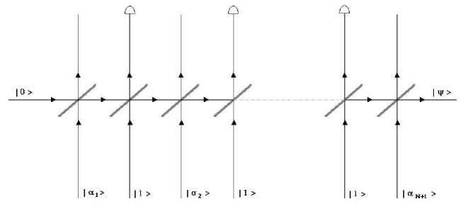
Figure 28: Experimental setup for the engineering of arbitrary states of a traveling-field mode. The array consists of $2N+1$ identical beam splitters all characterized by the same transmittance $\eta$. Coherent states $|\alpha_{i}\rangle$ and single-photon Fock states $|1\rangle$ in alternate sequence enter one input port of the beam splitters. The desired output state $|\Psi\rangle$ is prepared by a suitable choice of the coherent amplitudes $\alpha_{i}$.

Each two-step procedure corresponds to the action of a couple of beam splitters, and is repeated $N$ times. If, for all the two-step blocks, the photodiode detectors do not record photons, the two-step procedure supplies each block with the operation $a^{{\dagger}}\eta^{a^{{\dagger}}a}D(\alpha_{i})$ $(i=1,\ldots N)$, while the last ($2N+1$)-th beam splitter realizes the final displacement $D(\alpha_{N+1})$. Thus, with a certain probability, the output state is:

$$|\Psi\rangle\,\sim\,D(\alpha_{N+1})a^{{\dagger}}\eta^{a^{{\dagger}}a}D(\alpha_{N})a^{{\dagger}}\eta^{a^{{\dagger}}a}D(\alpha_{N-1})\cdots a^{{\dagger}}\eta^{a^{{\dagger}}a}D(\alpha_{1})|0\rangle\;.$$ (323)

Finally, it can be shown that the states (322) and (323) coincide for a suitable choice of the experimental parameters $\alpha_{i}$ $(i=1,\ldots N+1)$ [442]. This method has been proposed for the engineering of the reciprocal binomial states and of the polynomial states of the electromagnetic field [443, 444]. Fiurášek et al. have introduced an interesting variation of the scheme of Ref. [442]. At variance with the first proposal, in Ref. [445] the engineering of an arbitrary quantum state is achieved by repeated photon subtractions. This scheme is motivated by the fact that photon subtractions are experimentally much more practicable than photon additions. In their scheme the initial vacuum is replaced by a squeezed vacuum, and photon subtractions are realized by conditioned photodetections.

g)    Here we consider two other methods for the engineering of nonclassical states by means of multiphoton processes in nonlinear media. A first proposal is due to Leoński [446], and it is based on a set of models leading to the generation of quantum states that are very close to the coherent states of finite dimensional Hilbert spaces. The $(s+1)$-dimensional coherent states, finite dimensional approximations to the Glauber coherent states, have been defined in Refs. [447, 448]. They can be expressed in the standard form

$$|\alpha\rangle_{(s)}\,=\,\sum_{n=0}^{s}c_{n}^{(s)}|n\rangle\;,\quad\quad\,_{(s)}\langle\alpha|\alpha\rangle_{(s)}\,=\,\sum_{n=0}^{s}|c_{n}^{(s)}|^{2}\,=\,1\;,$$ (324)

where the coefficients $c_{n}^{(s)}$ have been numerically computed by Bužek et al. [447], and later analytically determined by Miranowicz et al. [448]. Leoński has shown that, starting from an initial vacuum state, superpositions very close to $|\alpha\rangle_{(s)}$ can be generated by suitable interactions between an external field and a nonlinear medium in a cavity[446].
The second proposal has been presented in Ref. [449] by A. Vidiella-Barranco and J. A. Roversi, and it is a generalization of the method introduced in Ref. [352]. The authors show that an arbitrary pure state $|\psi\rangle$, expressed in the Fock basis: $|\psi\rangle=\sum_{n=0}^{M}c_{n}|n\rangle$, can be obtained as the results of the unitary evolution generated by the Hamiltonian

$$H_{mph}^{M}\,=\,f_{0}(a^{{\dagger}}a)\,+\,\sum_{m=1}^{M}\frac{c_{m}}{\sqrt{m!}}[F(a^{{\dagger}}a)a^{m}\,+\,a^{{\dagger}m}F(a^{{\dagger}}a)]\;,$$ (325)

where

$$f_{0}(a^{{\dagger}}a)\,=\,c_{0}[2(1-a^{{\dagger}}a)F(a^{{\dagger}}a)-1]\;,\quad\quad F(a^{{\dagger}}a)\,=\,\sum_{l=0}^{M}A_{l}\;(a^{{\dagger}}a)^{l}\;.$$ (326)

The coefficients $A_{l}$ can be determined by the $M+1$ conditions $A_{0}=1$ and $1+pA_{1}+p^{2}A_{2}+...+p^{M}A_{M}=0$, with $p=1,...,M$. As an example, the state $|\psi_{2}\rangle=c_{0}|0\rangle+c_{2}|2\rangle$ can be generated by the Hamiltonian [449]

$$H_{2ph}^{2}\,=\,c_{0}[1-5a^{{\dagger}}a+4(a^{{\dagger}}a)^{2}-(a^{{\dagger}}a)^{3}]+\frac{c_{2}}{\sqrt{2}}[F(a^{{\dagger}}a)a^{2}+H.c.]\;,$$ (327)

$$F(a^{{\dagger}}a)\,=\,1-\frac{3}{2}a^{{\dagger}}a+\frac{1}{2}(a^{{\dagger}}a)^{2}\;,$$ (328)

which, however, would require, to be realized in nonlinear media, contributions from susceptibilities of very high order.

We conclude this Subsection by briefly mentioning some more recent proposals of quantum state engineering. A scheme based on the use of conditional measurements on entangled twin-beams to produce and manipulate nonclassical states of light has been investigated in Ref. [450]. Another proposal has been presented in Ref. [451] in order to engineer squeezed cavity-field states via the interaction of the cavity field with a driven three-level atom. Finally, the high nonlinearities available in the electromagnetically induced transparency regime offer further possibilities to quantum state engineering. For example, in Ref. [452] the generation of entangled coherent states via the cross-phase-modulation effect has been carefully analyzed.

5.11 Nonclassicality of a state: criteria and measures

Although a universal criterion for detecting nonclassicality of a quantum state is a somewhat elusive concept, in this Subsection we will discuss some interesting proposals aimed at qualifying and quantifying nonclassicality, limiting our attention to single-mode states of the radiation field. As we have already seen, the concept of nonclassicality of a state of the radiation field is generally associated with some emerging physical property with no classical counterpart. Typically, nonclassicality can be measured in a variety of ways, e.g. by computing the degree of squeezing [187, 215, 403, 453]; by observing the sub-Poissonian behavior of the statistics [41, 454] or the presence of oscillations in the photon number distribution [455]; and by investigating the non-existence or the negativity of the phase-space quasi-probability distributions [15, 46]. Besides these traditional and useful tests, many other types of indicators, conditions, and measures highlighting different nonclassical signatures, have been introducedin the literature. Among the most interesting, we mention the distance of a considered state to a set of reference states (e.g. the coherent states) [456, 457, 458, 459]; some peculiar behaviors of quasi-probability distributions or characteristic functions [46, 460, 461, 462, 463, 464, 465]; the violation of inequalities involving the moments of the annihilation and creation operators [273, 466, 467, 468, 469, 470, 471]; and, finally, the violation of inequalities involving the characteristic functions [472, 473].
The definition of a nonclassical distance in the domain of quantum optics has been introduced by Hillery [456]. Such a distance $\delta_{H}(\rho,\rho_{cl})$ of a certain state $\rho$ from a set of reference classical states $\rho_{cl}$ is defined as

$$\delta_{H}(\rho,\rho_{cl})=\inf_{\rho_{cl}}\parallel\rho-\rho_{cl}\parallel_{1}\,,$$ (329)

where $\rho_{cl}$ ranges over all classical density matrices and $\parallel\cdot\parallel_{1}$ denotes the (trace) norm of an operator:

$$\parallel A\parallel_{1}=Tr[|A|]=Tr[(A^{{\dagger}}A)^{1/2}]\,,$$ (330)

for a generic operator $A$. Following the path opened by Hillery, other distances have been considered to define computable indicators of nonclassicality. For instance, the Hilbert-Schmidt distance $d_{HS}$

$$d_{HS}(\rho,\rho_{cl})=\parallel\rho-\rho_{cl}\parallel_{2}=\{Tr[(\rho-\rho_{cl})^{2}]\}^{1/2}\;,$$ (331)

has been used to define the following measure of nonclassicality [457]:

$$\delta_{HS}(\rho,\rho_{cl})=\min_{\rho_{cl}}d_{HS}(\rho,\rho_{cl})\;.$$ (332)

The Bures distance $d_{B}(\rho,\rho_{cl})$ [474] is defined as

$$d_{B}(\rho,\rho_{cl})=\left\{2-2\sqrt{\mathcal{F}(\rho,\rho_{cl})}\right\}^{1/2}\;,$$ (333)

where

$$\mathcal{F}(\rho,\rho_{cl})=\{Tr[(\sqrt{\rho}\,\rho_{cl}\,\sqrt{\rho})^{1/2}]\}^{2}\;.$$ (334)

The Bures distance has been exploited in Ref. [458] to introduce a measure of nonclassicality of the form

$$\delta_{B}^{2}(\rho,\rho_{cl})=\min_{\rho_{cl}}\frac{1}{2}d_{B}^{2}(\rho,\rho_{cl})\;.$$ (335)

The quantity in Eq. (335) is obviously more difficult to compute compared to measures based on the trace norm of operators. We should finally mention that in phase space it is possible to define a further distance-based measure of nonclassicality, the so-called Monge distance between the Husimi distribution of the chosen state and that of the reference coherent state [459].
A very interesting approach to the detection, and even to the measurement, of the nonclassicality of a state is based on the behavior of the corresponding quasi-probability distributions or characteristic functions in phase space. A nonclassical depth in phase space can be defined by introducing a proper distribution $R$ interpolating between the $P$- and the $Q$- functions [461]

$$R(\alpha,\tau)=\frac{1}{\pi\tau}\int d^{2}w\exp\left\{-\frac{1}{\tau}|\alpha-w|^{2}\right\}P(w)\;,$$ (336)

where $\tau$ is a continuous parameter (for $\tau=0,\,1/2,\,1$ the distribution $R$ reduces to the $P$-, $W$-, and $Q$- function, respectively). The nonclassical depth $\tau_{ncl}$ is defined as the lower bound of the set of values of $\tau$ that lead to a smoothing of the $P$-function of a quantum state. It turns out that $\tau_{ncl}=0$ for a coherent state, $\tau_{ncl}=(e^{2r}-1)/2e^{2r}$ for a squeezed state ($r$ being the squeezing parameter), and $\tau_{ncl}=1$ for a number state [461]; this finding gives support to the validity of $\tau_{ncl}$ as an estimator of nonclassicality. According to Lütkenhaus and Barnett [462], a quantitative measure of nonclassicality can be associated with the $p$ parameter of the $p$-ordered phase-space distributions $W(\alpha,\,p)$ (see Eq. (43)). In fact, two quasi-probability distributions for the same state but different values of $p$ are related by a convolution of the form

$$W(\alpha,\,p^{\prime})=\int d^{2}\beta\;W(\beta,\,p^{\prime\prime})\frac{2}{\pi(p^{\prime\prime}-p^{\prime})}\exp\left\{-\frac{2|\alpha-\beta|^{2}}{p^{\prime\prime}-p^{\prime}}\right\}\;,$$ (337)

with $p^{\prime\prime}>p^{\prime}$. Eq. (337) can be viewed as the solution to a sourceless diffusion equation with $p$, playing the role of backward time: in fact $W(\alpha,\,p)$ is smoothed in the direction of decreasing $p$. The critical value of $p$ for which the boundary of the well-behaved quasi-probability distributions is reached, can be assumed as a measure of nonclassicality [462]. Probably the most intuitive indicator of nonclassicality for a quantum state $|\psi\rangle$ is the one based on the volume of the negative part of the Wigner function [46, 460]:

$$\delta_{\psi}=\int\int dx_{\theta}\,dp_{\theta}\;|W_{\psi}(x_{\theta},p_{\theta})|-1\;,$$ (338)

where $W_{\psi}(x_{\theta},p_{\theta})$ is the Wigner function corresponding to the state $|\psi\rangle$ in the quadrature representation. A further phase space related criterion has been introduced by Vogel, who has proposed to define that a quantum state is nonclassical if the modulus of its characteristic function exceeds that of the vacuum state at all points in the space of definition [464]. This definition has been used to verify experimentally, via quantum tomographic reconstruction, the nonclassical nature of statistical mixtures of the vacuum state $|0\rangle$ and of the single-photon Fock state $|1\rangle$ [465]. Unfortunately, it has been shown that some nonclassical states violate this criterion [475].
Another different typology of criteria is based on hierarchies of inequalities involving the statistical moments of the annihilation and creation operators $a$ and $a^{{\dagger}}$. Agarwal and Tara have introduced sufficient conditions for nonclassicality based on the moments of the photon number operator [273]. The starting point is the diagonal coherent state expansion of the density matrix $\rho$

$$\rho=\int d^{2}\alpha\,P(\alpha)|\alpha\rangle\langle\alpha|\;.$$ (339)

Recalling the definition given in Section 2, a state $\rho$ is said to be ”classical” if the $P$-function is pointwise nonnegative, and nowhere more singular than a $\delta$-function (that is a classical behavior of the $P$-function as a probability density). Let us now consider a Hermitian operatorial function $\hat{F}_{n}(a^{{\dagger}},a)$ of normally ordered creation and annihilation operators, i.e. $\langle\alpha|\hat{F}_{n}(a^{{\dagger}},a)|\alpha\rangle=F_{n}(\alpha^{*},\alpha)$. The quantum mechanical expectation value of $\hat{F}_{n}$ in the state $\rho$ is

$$\langle\hat{F}_{n}\rangle=Tr[\rho\hat{F}_{n}]=\int d^{2}\alpha\,P(\alpha)F_{n}(z^{*},z)\;.$$ (340)

The state $\rho$ is then defined to be nonclassical if $\langle\hat{F}_{n}\rangle<0$ (”quantum negativity”) for some $F_{n}(z^{*},z)\geq 0$. Let us choose

$$\hat{F}_{n}(a^{{\dagger}},a)=\sum_{r,s=0}^{n-1}c_{r}^{*}c_{s}\,a^{{\dagger}(r+s)}a^{(r+s)}\;,$$ (341)

with $c_{k}$ arbitrary constants, and let us define $m^{(k)}=\langle a^{{\dagger}k}a^{k}\rangle$. Then, if $P(\alpha)$ behaves like a classical distribution, the following quadratic form in the constants $\{c_{k}\}$:

$$F_{n}(\{c_{k}\})=\sum_{r,s=0}^{n-1}c_{r}^{*}c_{s}\,m^{(r+s)}\;,$$ (342)

should be positive, thus implying the positivity of the matrix

$$M_{n}=\left(\begin{array}[]{ccccc}1&m^{(1)}&m^{(2)}&\cdots&m^{(n-1)}\\ m^{(1)}&m^{(2)}&m^{(3)}&\cdots&m^{(n)}\\ m^{(2)}&m^{(3)}&m^{(4)}&\cdots&m^{(n+1)}\\ \vdots&\vdots&\vdots&\ddots&\vdots\\ m^{(n-1)}&m^{(n)}&m^{(n+1)}&\cdots&m^{(2n-2)}\\ \end{array}\right)\;.$$ (343)

It is easy to check that for $n=2$ the condition $M_{2}>0$ reduces to the condition of positivity of the Mandel $Q$ parameter Eq. (41). For $n>2$ we get conditions on higher order moments, that are needed for the full characterization of non-Gaussian states. An example of such states is the photon-added thermal state, described by the density operator $\rho_{add-th}\propto a^{{\dagger}m}e^{-\beta a^{{\dagger}}a}a^{m}$ $(\beta>0)$, that exhibits neither squeezing nor sub-Poissonian statistics in some ranges of the inverse temperature $\beta$. In order to test the nonclassicality of $\rho_{add-th}$, one can for instance invoke the negativity of the matrix $M_{3}$. To this aim one can introduce the following numerical form, bounded from below by $-1$ [273]:

$$A_{3}=\frac{\det M_{3}}{\det W_{3}-\det M_{3}}\;,$$ (344)

where the matrix $W_{n}$ is constructed as $M_{n}$ with the replacement $m^{(n)}\rightarrow w^{(n)}=\langle(a^{{\dagger}}a)^{n}\rangle$. The condition $A_{3}<0$ determines the region of nonclassicality, and it can be shown that for the state $\rho_{add-th}$ there exist ranges of $\beta$ such that $A_{3}<0$ even in the absence of squeezing and sub-Poissonian statistics. The nonclassical nature of a superposition of coherent states can be also tested in a similar way [273]. Different versions and generalizations of this criterion have been given in Refs. [466, 467].
Among all the possible Hermitian operatorial functions $\hat{F}_{n}(a^{{\dagger}},a)$ of normally ordered creation and annihilation operators, one can consider the set of phase invariant (number conserving) operators, i.e. the ones such that $[\hat{F}_{n},a^{{\dagger}}a]=0$. Arvind et al. have introduced a phase-averaged $P$-function [468]

$$\mathcal{P}(I)=\int_{0}^{2\pi}\frac{d\theta}{2\pi}P(I^{1/2}e^{i\theta})\;.$$ (345)

From definition Eq. (345), the quantities $\langle\hat{F}_{n}\rangle$ can be written as

$$\langle\hat{F}_{n}(a^{{\dagger}},a)\rangle=\int_{0}^{\infty}dI\,\mathcal{P}(I)\,F_{n}(I^{1/2},I^{1/2})\;.$$ (346)

By requiring the nonnegativity of the expectations values (346) for a classical state, then the following finer definition of nonclassicality can be stated [468]: a quantum state $\rho$ is weakly nonclassical if $\mathcal{P}(I)\geq 0$, but $P(\alpha)\ngeq 0$; and strongly nonclassical if also the quantity $\mathcal{P}(I)$ ceases to be a probability distribution, that is: $\mathcal{P}(I)\ngeq 0$, and $P(\alpha)\ngeq 0$. D’Ariano et al. have proposed an experimental test of these conditions by exploiting homodyne tomography [469], taking into account also imperfect quantum efficiency of the homodyne detection. Along the same line followed in Refs. [273, 468] very recent criteria of nonclassicality, constructed as an infinite series of inequalities, have been formulated in terms of normally ordered moments of the annihilation and creation operators [470, 471]. Let us briefly outline the method to derive these conditions. Let $\hat{f}(a^{{\dagger}},a)$ be an operatorial function whose normally ordered form exists. The occurrence of negative mean values of the form

$$\langle:\hat{f}^{{\dagger}}\hat{f}:\rangle=\int d^{2}\alpha\,|f(\alpha)|^{2}P(\alpha)\;<0\,$$ (347)

is a signature of nonclassicality. The condition (347) also implies the violation of the Bochner theorem for the existence of a classical characteristic function [476] (a characteristic function $\chi(z,w)$, satisfying the condition $\chi(0,0)=1$, is a classical characteristic function if and only if it is positive semidefinite). If $\hat{f}$ is chosen as

$$\hat{f}(a^{{\dagger}},a)=\sum_{k=0}^{K}\sum_{l=0}^{L}c_{kl}\,a^{{\dagger}k}a^{l}\,,$$ (348)

with arbitrary constants $c_{kl}$, then, for a classical state, the quadratic form

$$\langle:\hat{f}^{{\dagger}}\hat{f}:\rangle=\sum_{k,r=0}^{K}\sum_{l,s=0}^{L}c_{rs}^{*}c_{kl}\,\langle a^{{\dagger}l+r}a^{k+s}\rangle\,,$$ (349)

should be positive. Equivalently, the condition for the classicality of a state is provided by the positivity of a hierarchy of determinants $d_{N}$ of square matrices of dimension $N\times N$ (where $N=K+L$, and $K$, $L$ arbitrary) of the form:

$$d_{N}=\left|\begin{array}[]{ccccccc}1&\langle a\rangle&\langle a^{{\dagger}}\rangle&\langle a^{2}\rangle&\langle a^{{\dagger}}a\rangle&\langle a^{{\dagger}2}\rangle&\cdots\\ \langle a^{{\dagger}}\rangle&\langle a^{{\dagger}}a\rangle&\langle a^{{\dagger}2}\rangle&\langle a^{{\dagger}}a^{2}\rangle&\langle a^{{\dagger}2}a\rangle&\langle a^{{\dagger}3}\rangle&\cdots\\ \langle a\rangle&\langle a^{2}\rangle&\langle a^{{\dagger}}a\rangle&\langle a^{3}\rangle&\langle a^{{\dagger}}a^{2}\rangle&\langle a^{{\dagger}2}a\rangle&\cdots\\ \langle a^{{\dagger}2}\rangle&\langle a^{{\dagger}2}a\rangle&\langle a^{{\dagger}3}\rangle&\langle a^{{\dagger}2}a^{2}\rangle&\langle a^{{\dagger}3}a\rangle&\langle a^{{\dagger}4}\rangle&\cdots\\ \langle a^{{\dagger}}a\rangle&\langle a^{{\dagger}}a^{2}\rangle&\langle a^{{\dagger}2}a\rangle&\langle a^{{\dagger}}a^{3}\rangle&\langle a^{{\dagger}2}a^{2}\rangle&\langle a^{{\dagger}3}a\rangle&\cdots\\ \langle a^{2}\rangle&\langle a^{3}\rangle&\langle a^{{\dagger}}a^{2}\rangle&\langle a^{4}\rangle&\langle a^{{\dagger}}a^{3}\rangle&\langle a^{{\dagger}2}a^{2}\rangle&\cdots\\ \cdots&\cdots&\cdots&\cdots&\cdots&\cdots&\cdots\\ \end{array}\right|\;.$$ (350)

By this procedure one can prove that a state is nonclassical if and only if at least one of the determinants satisfies [471]

$$d_{N}<0\;,$$ (351)

with $N>2$, because $d_{2}$ represents the incoherent part of the photon number $\langle a^{{\dagger}}a\rangle-\langle a^{{\dagger}}\rangle\langle a\rangle$ which is always nonnegative and thus cannot be used as a quantifier of nonclassicality. It is possible to provide other sufficient conditions for nonclassicality by considering subdeterminants of $d_{N}$ obtained by deleting pairs of lines and columns that cross at a diagonal element of the matrix. Refs. [471, 473] investigate the connection between nonclassicality criteria, the quantumness of a state, and the 17th Hilbert problem [477]. The latter states that not every positive semidefinite polynomial must be a sum-of-squares of other polynomials.
We finally wish to mention another very interesting approach that relates the nonclassicality of a single-mode quantum state to the amount of two-mode entanglement that can be generated by doubling the original field mode through linear optical elements (beam splitters), auxiliary classical states, and ideal photodetectors [478].

6 Canonical multiphoton quantum optics

In Section 5 we have reviewed several interesting approaches sharing a common goal: the generalization of two-photon interactions to multiphoton processes associated to higher order nonlinearities, for the engineering of multiphoton nonclassical states of the electromagnetic field. However relevant in various aspects, all these methods fail in extending the elegant canonical formalism of two-photon processes, that, via the linear Bogoliubov transformation (or the equivalent unitary squeezing operator) determines completely the physical and mathematical structure of two-photon quantum optics, including the diagonalizable two-photon Hamiltonians, the corresponding normal modes, and the exactly computable two-photon squeezed states. Inspired by its power and generality, recently a series of papers has appeared, that generalizes the canonical formalism to multiphoton quantum optics [479, 480, 481, 482, 483]. This generalized canonical formalism has been constructed both for one mode [479, 481], and for two modes [480] of the electromagnetic field. For single-mode systems the canonical structure has been determined by introducing canonical transformations that depend on generic nonlinear functions of the homodyne combinations of pairs of canonically conjugated quadratures [479]. This homodyne canonical formalism defines the class of the single–mode, homodyne multiphoton squeezed states (HOMPSS), which include the single–mode, single–quadrature multiphoton squeezed states as a particular case [481, 482]. The nonlinear canonical formalism has been extended to define two-mode multiphoton nonclassical states [480]. This further generalization is achieved by introducing canonical two-mode transformations that depend on nonlinear functions of heterodyne variables [57, 58]. The corresponding canonical structure, strictly related to the entangled state representation [484, 485, 486], defines highly nonclassical, two-mode entangled states, the heterodyne multiphoton squeezed states (HEMPSS). A very nice feature of canonical multiphoton quantum optics is that the canonical transformations depend in general on tunable physical parameters. In the case of HOMPSS, the adjustable parameter is the local-oscillator mixing angle. In the case of HEMPSS, there may be several adjustable quantities, as will be discussed in detail in the following. The existence of free parameters allows to arbitrarily vary the statistics of the states and to interpolate between different Hamiltonian models of multiphoton processes. Finally, one can envisage relatively simple and in principle feasible experimental schemes for the production of multiphoton nonclassical states in nonlinear media by realizing elementary interaction models based on the nonlinear canonical structure [480].

6.1 One-mode homodyne multiphoton squeezed states: definitions and statistical properties

In this Subsection we describe the single-mode, nonlinear canonical transformations [479], introduce the definition of the HOMPSS, and discuss the main aspects of the formalism. We generalize the one-mode, linear two-photon Bogoliubov transformation by defining a quasi-photon operator $b$ of the form

$$b\,=\,{\tilde{\mu}}a_{\theta}\,+\,{\tilde{\nu}}a_{\theta}^{\dagger}\,+\,\gamma F(X_{\theta})\;,\quad\quad X_{\theta}\,=\,\frac{a_{\theta}+a_{\theta}^{\dagger}}{\sqrt{2}}\;,$$ (352)

where $\tilde{\mu}$, $\tilde{\nu}$, and $\gamma$ are generic complex parameters, $a_{\theta}=e^{-i\theta}a$ is the rotated annihilation operator, and $F$ is an arbitrary hermitian nonlinear function of the homodyne quadrature observable $X_{\theta}=X\cos{\theta}+P\sin{\theta}$ (where $X$ and $P$ are the original quadrature observables). The transformation is canonical, namely $[b,b^{{\dagger}}]=1$, if the parameters satisfy

$$|\tilde{\mu}|^{2}-|\tilde{\nu}|^{2}\,=\,1\;,\quad\quad\quad Re[{\tilde{\mu}}\gamma^{*}-{\tilde{\nu}}^{*}\gamma]\,=\,0\;.$$ (353)

The first condition in Eq. (353) correctly reproduces the constraint corresponding to the linear Bogoliubov transformation. Remarkably, the additional condition in Eq. (353) does not depend on the specific choice of the nonlinear function $F$, but only on its strength $\gamma$. The first contraint is automatically satisfied with the standard parametrizations ${\tilde{\mu}}\equiv e^{i\theta}\mu=e^{i\theta}\cosh r$, ${\tilde{\nu}}\equiv e^{-i\theta}\nu=e^{i(\phi-\theta)}\sinh r$. Writing $\gamma=|\gamma|e^{i\delta}$, the second constraint in Eq. (353) is then recast in the two (equivalent) forms

$$\cosh r\cos(\delta-\theta)\,-\,\sinh r\cos(\delta+\theta-\phi)\,=\,0\;,$$ (354)

$$\tan\left(\delta-\frac{\phi}{2}\right)\tan\left(\theta-\frac{\phi}{2}\right)\,=\,-e^{-2r}\;.$$ (355)

The form (354) suggests immediately, by imposing the vanishing of the trigonometric functions, one exact solution that preserves the freedom on the choice of the squeezing parameter $r$:

$$\delta-\theta\,=\,\pm\frac{\pi}{2}\;,\quad\quad\quad\delta+\theta-\phi\,=\,\pm\frac{\pi}{2}\;.$$ (356)

Alternatively, the second form (355) allows to determine, in general numerically, all the possible solutions, either by constraining the squeezing parameter $r$ alone, or only one of the phases.
We denote by $|\beta,\gamma\rangle_{b}$ the generalized coherent states associated with the transformation (352), defined as the eigenstates of the transformed annihilation operator $b$:

$$b\,|\beta,\gamma\rangle_{b}\,=\,\beta\,|\beta,\gamma\rangle_{b}\;,$$ (357)

where $\beta$ is a generic complex number $\beta\,=\,|\beta|e^{i\varsigma}$. The solutions of Eq. (357) define, in a sense that will become clear in the following, the (one-mode) homodyne multiphoton squeezed states, or HOMPSS in short. In the rotated quadrature representation $\{|x_{\theta}\rangle\}$, their wave function reads

$$\psi_{\beta,\gamma}(x_{\theta}) \,=\,\langle x_{\theta}|\beta,\gamma\rangle_{b}\,=$$ (358)

$$\pi^{-1/4}\left(Re\left[\frac{{\tilde{\mu}}+{\tilde{\nu}}}{{\tilde{\mu}}-{\tilde{\nu}}}\right]\right)^{1/4}\exp\left\{-\frac{1}{2}|\beta|^{2}-\frac{1}{2}\frac{{\tilde{\mu}}^{*}-{\tilde{\nu}}^{*}}{{\tilde{\mu}}-{\tilde{\nu}}}\beta^{2}\right\}$$

$$\times\exp\left\{-\frac{1}{2}\frac{{\tilde{\mu}}+{\tilde{\nu}}}{{\tilde{\mu}}-{\tilde{\nu}}}\,x_{\theta}^{2}+\frac{\sqrt{2}\beta}{{\tilde{\mu}}-{\tilde{\nu}}}\,x_{\theta}\right\}$$

$$\times\exp\left\{-\frac{\sqrt{2}\gamma}{{\tilde{\mu}}-{\tilde{\nu}}}\int^{x_{\theta}}F(y)dy\right\}\;,$$

where, due to the canonical conditions (353), the coefficient which multiplies the integral in the last exponential is purely imaginary, thus ensuring normalizability. We thus see that the effect of the nonlinearity, namely the presence of multiphoton interactions, amounts to the appearance of a non Gaussian phase factor in the wave function.
For the special choices $\theta=0\,,\,\frac{\pi}{2}$ the HOMPSS reduce to single-mode, single-quadrature multiphoton squeezed states [481, 482]. Of course, for $\gamma=0$ the expression (358) reduces to the Gaussian wave function of the two-photon squeezed states. The HOMPSS can be also obtained from the vacuum state by applying on it a compound unitary transformation:

$$|\beta,\gamma\rangle_{b}\,=\,U_{\theta}(X_{\theta})\,D_{\theta}(\alpha_{\theta})\,S_{\theta}(\zeta_{\theta})\,|0\rangle\;,$$ (359)

where $D_{\theta}(\alpha_{\theta})\,=\,\exp\left(\alpha_{\theta}a^{{\dagger}}_{\theta}-\alpha^{*}_{\theta}a_{\theta}\right)$ is the standard Glauber displacement operator with $\alpha_{\theta}\,=\,{\tilde{\mu}}^{*}\beta-\tilde{\nu}\beta^{*}$. Next, $S_{\theta}(\zeta_{\theta})\,=\,\exp\left(-\frac{\zeta_{\theta}}{2}a^{{\dagger}2}_{\theta}+\frac{\zeta_{\theta}^{*}}{2}a^{2}_{\theta}\right)$ is the squeezing operator with $\zeta_{\theta}\,=\,re^{i(\phi-2\theta)}$, and, finally,

$$U_{\theta}(X_{\theta})\,=\,\exp\left[-\frac{\sqrt{2}\gamma}{{\tilde{\mu}}-{\tilde{\nu}}}\int^{X_{\theta}}dYF(Y)\right]$$

is the unitary, linear operator of “nonlinear mixing”, which is responsible for the non Gaussian part of the HOMPSS, and is a consequence of the associated multiphoton nonlinear processes. The expression (359) shows, once more, that the HOMPSS are a generalization of the two-photon squeezed states for nonvanishing nonlinear strength $\gamma$, and smoothly reduce to them in the limit $\gamma\rightarrow 0$. The HOMPSS admit resolution of the unity

$$\mathbb{I}_{b}\,=\,\frac{1}{\pi}\int d^{2}\beta|\beta,\gamma\rangle_{b}\;{}_{b}\langle\beta,\gamma|\;,$$ (360)

and are nonorthogonal

$$\,{}_{b}\langle\beta_{1},\gamma|\beta_{2},\gamma\rangle_{b}\,=\,\exp\left\{-\frac{1}{2}|\beta_{1}|^{2}-\frac{1}{2}|\beta_{2}|^{2}+\beta_{1}^{*}\beta_{2}\right\}\;.$$ (361)

Therefore, they constitute an overcomplete basis.
The nonlinear unitary transformation (352) can be inverted; in fact, by using conditions (353),

$$a_{\theta}\,=\,\tilde{\mu}^{*}b-\tilde{\nu}b^{{\dagger}}-(\tilde{\mu}^{*}\gamma-\tilde{\nu}\gamma^{*})F(X_{\theta})\;,$$

$$X_{\theta}\,=\,\frac{1}{\sqrt{2}}[(\tilde{\mu}^{*}-\tilde{\nu}^{*})b+(\tilde{\mu}-\tilde{\nu})b^{{\dagger}}]\;.$$ (362)

These inversion formulae allow the exact computation of all the physically important statistical quantities, in particular, the expectation values of all the operatorial functions of the form $\sum c_{nm}a^{{\dagger}n}a^{m}$, for any arbitrary choice of the coefficients $c_{nm}$.
For the uncertainties on the conjugate homodyne quadratures $X_{\theta}$ and $P_{\theta}=-i(a_{\theta}-a_{\theta}^{\dagger})/\sqrt{2}$ in a generic HOMPSS, one finds:

$$\langle\Delta^{2}X_{\theta}\rangle \,=\,\frac{1}{2}|\tilde{\mu}-\tilde{\nu}|^{2}\;,$$ (363)

$$\langle\Delta^{2}P_{\theta}\rangle \,=\,\frac{1}{2}|\tilde{\mu}+\tilde{\nu}|^{2}+2Im^{2}[{\tilde{\mu}}^{*}\gamma-\tilde{\nu}\gamma^{*}](\langle F^{2}\rangle_{\beta}-\langle F\rangle_{\beta}^{2})$$

$$-2Im[{\tilde{\mu}}^{*}\gamma-\tilde{\nu}\gamma^{*}]Im[(\tilde{\mu}+\tilde{\nu})\langle[F,b^{{\dagger}}]\rangle_{\beta}]\;,$$ (364)

where $\langle\cdot\rangle_{\beta}$ denotes the expectation value in the HOMPSS $|\beta,\gamma\rangle_{b}$. From these expressions one can compute the general form of the uncertainty product for a generic choice of the nonlinear function $F$. However, at this point, the explicit expression for a specific example can be illuminating. As in Ref. [479], we consider the case of the lowest possible nonlinearity

$$F(X_{\theta})\,=\,X_{\theta}^{2}\;.$$ (365)

In this case, choosing the optimal solutions of the canonical constraints (356), and using the expressions (363), (364), we obtain the following explicit form of the uncertainty product

$$\langle\Delta^{2}X_{\theta}\rangle\langle\Delta^{2}P_{\theta}\rangle\,=\,\frac{1}{4}\,+\,\frac{1}{2}|\gamma|^{2}e^{-4r}\{1+4|\beta|^{2}+4|\beta|^{2}\cos 2[\varsigma-\theta]\}\;,$$ (366)

where we recall that $\varsigma$ denotes the phase of $\beta$. The r.h.s. in Eq. (366) attains its minimum value for $\varsigma-\theta\,=\,\pm\frac{\pi}{2}\;$:

$$\langle\Delta^{2}X_{\theta}\rangle\langle\Delta^{2}P_{\theta}\rangle\,=\,\frac{1}{4}\,+\,\frac{1}{2}|\gamma|^{2}e^{-4r}\;.$$ (367)

Therefore, either by assuming a very weak strength $|\gamma|$ of the nonlinearity, and/or a sufficiently high squeezing $r$, we see that the HOMPSS are to all practical purposes minimum uncertainty states.

In order to analyze the statistical properties of the HOMPSS, we assume the particular solution (356) for the canonical conditions (354), and adopt the minimal quadratic form (365) for the nonlinear function $F$. The average photon number $\langle n\rangle\,=\,\,_{b}\langle\beta,\gamma|n|\beta,\gamma\rangle_{b}$, in the original mode variables $(n\,=\,a^{{\dagger}}a)$, can be easily computed by exploiting the inversion formulae (362). In Fig. (29) (a) we show $\langle n\rangle$ as a function of the homodyne phase $\theta$, with $r=0.5$, $\beta=3$, and for different values of the nonlinear strength $|\gamma|$.

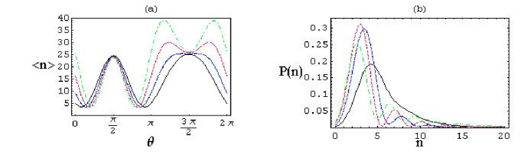
Figure 29: (a) The mean photon number $\langle n\rangle$ as a function of the homodyne angle $\theta$, for a HOMPSS with $r=0.5$, $\beta=3$, and nonlinear strengths: $|\gamma|=0$ (full line); $|\gamma|=0.1$ (dotted line); $|\gamma|=0.2$ (dashed line); and $|\gamma|=0.4$ (dot-dashed line). (b) The photon number distribution $P(n)$ for a HOMPSS with $\theta=\frac{\pi}{6}$, and with the same choices of (a) for $r$, $\beta$, and $|\gamma|$ (with the same plot styles). In plots (a) and (b) the HOMPSS are associated to the canonical conditions $\delta-\theta=-\frac{\pi}{2}$, $\delta+\theta-\phi=-\frac{\pi}{2}$.

We see that the average photon number is strongly dependent on $|\gamma|$; however, it is the homodyne phase $\theta$ that plays the main role in determining the variation of $\langle n\rangle$. In Fig. (29) (b) we plot the photon number distribution

$$P(n)\,\equiv\,|\langle n|\beta,\gamma\rangle_{b}|^{2}\,=\, \left|\int dx_{\theta}\langle n|x_{\theta}\rangle\langle x_{\theta}|\beta,\gamma\rangle_{b}\right|^{2}\,=$$

$$=\, \frac{1}{2^{n}n!\pi^{1/2}}\left|\int dx_{\theta}e^{-\frac{x_{\theta}^{2}}{2}}H_{n}(x_{\theta})\psi_{\beta,\gamma}(x_{\theta})\right|^{2}\;,$$ (368)

for $\theta=\frac{\pi}{6}$, where $H_{n}(x_{\theta})$ denotes the Hermite polynomial of degree $n$. The distribution $P(n)$ shows an oscillatory behavior, which is more pronounced for increasing $|\gamma|$. In Fig. (30) (a) we plot the second order correlation function as a function of $r$, and in Fig. (30) (b) the second order correlation function as a function of $\theta$, in both cases for different values of the nonlinear strength $|\gamma|$.

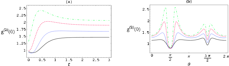
Figure 30: (a) Plot of the second order correlation function $g^{(2)}(0)$, as a function of $r$, for a HOMPSS with $\beta=3$, $\theta=\frac{\pi}{3}$, and nonlinear strengths: $|\gamma|=0.1$ (full line); $|\gamma|=0.2$ (dotted line); $|\gamma|=0.3$ (dashed line); and $|\gamma|=0.4$ (dot-dashed line). (b) Plot of $g^{(2)}(0)$, as function of $\theta$, for a HOMPSS with $\beta=3$, $r=0.5$, and for the same values of $|\gamma|$ (with the same plot styles). In plots (a) and (b) the HOMPSS are associated to the canonical conditions $\delta-\theta=-\frac{\pi}{2}$, $\delta+\theta-\phi=\frac{\pi}{2}$.

Fig. (30) (a) shows that the correlation function, at fixed $\theta$, exhibits a typical behavior: as the degree of squeezing $r$ is increased, it tends to a costant asymptote whose numerical value increases with increasing $|\gamma|$. Fig. (30) (b) shows instead that the dependence of the correlation function on the homodyne angle $\theta$ is so strong that, as the latter is varied, the nature of the statistics can change, and one can thus select super- or sub-Poissonian regimes. The strong and flexible nonclassical character of the HOMPSS can be further verified by determining their Wigner quasi-probability distribution (45) for the classical phase space variables $x_{\theta}$ and $p_{\theta}$ corresponding to the canonically conjugate orthogonal quadrature components $X_{\theta}$ and $P_{\theta}$. Figures (31) (a) and (b) show, respectively, a global projection of $W(x_{\theta},p_{\theta})$, and an orthogonal section $W(x_{\theta}=x_{0},p_{\theta})$ with $x_{0}=0$. The two plots show that the Wigner function of canonical multiphoton squeezed states exhibits nonclassical features, beyond a squeezed shape, that are in general much stronger than those of the corresponding canonical two-photon squeezed states, including interference fringes and negative values.

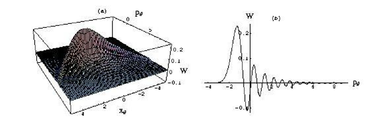
Figure 31: (a) The Wigner function $W(x_{\theta},p_{\theta})$ for a HOMPSS with $r=1.0$, $\beta=3$, $|\gamma|=0.5$, and $\theta=\frac{\pi}{2}$. (b) Section of the Wigner function $W(x_{\theta}=x_{0},p_{\theta})$, with $x_{0}=0$. The canonical conditions $\delta-\theta=-\frac{\pi}{2}$, $\delta+\theta-\phi=\frac{\pi}{2}$ have been assumed.

6.2 Homodyne multiphoton squeezed states: diagonalizable Hamiltonians and unitary evolutions

In this Subsection we discuss the multiphoton Hamiltonians and the multiphoton processes which can be associated to the one-mode nonlinear canonical transformations that we have introduced. We will then show how to determine the associated exact, unitary time-evolutions.

The most elementary multiphoton interaction which can be associated with the nonlinear transformation (352) is defined by the diagonal Hamiltonian

$$H_{1}^{diag}\,=\,b^{{\dagger}}b\;.$$

The evolved state $|\psi(t)\rangle=e^{-itH_{1}^{diag}}|in\rangle$, generated by the action of Hamiltonian $H_{1}^{diag}$ on a generic initial state $|in\rangle$, can be easily determined by using the overcomplete set of states $\{|\beta,\gamma\rangle_{b}\}$. In fact, one can insert in the expression for $|\psi(t)\rangle$ the completeness relation (360): $|\psi(t)\rangle=e^{-itH_{1}^{diag}}\mathbb{I}_{b}|in\rangle$, and exploit the eigenvalue equation (357). For the choice (365), the Hamiltonian $H_{1}^{diag}$, expressed in terms of the original mode operators $a$ and $a^{{\dagger}}$, takes the form

$$H_{1G}^{4ph}\,=\, A_{0}+(A_{1}a^{{\dagger}}+A_{2}a^{{\dagger}2}+A_{3}a^{{\dagger}3}+A_{4}a^{{\dagger}4}+H.c.)$$ (369)

$$+\,B_{0}a^{{\dagger}}a+B_{1}a^{{\dagger}2}a^{2}+(Ca^{{\dagger}2}a+Da^{{\dagger}3}a+H.c.)\;.$$

We see that $H_{1G}^{4ph}$ contains all the $n$-photon processes up to $n=4$. That is, Eq. (369) contains the one-, two-, three-, and four-photon down conversion terms $a^{{\dagger}n}$ $(n=1,...,4)$, the Kerr term $a^{{\dagger}2}a^{2}$, and the terms $a^{{\dagger}2}a$ and $a^{{\dagger}3}a$. The two last terms can be interpreted as higher order one- and two-photon interactions modulated by the intensity $a^{{\dagger}}a$, or, as energy-assisted one-photon and two-photon hopping terms. Obviously, it would be important that the exactly diagonalizable Hamiltonians constructed in terms of the transformed mode $b$ describe realistically feasible multiphoton processes. To this aim, it is crucial to have a sufficiently large number of tunable parameters which can model the multiphoton Hamiltonians. Therefore, one can generalize the “free” Hamiltonian $H_{1}^{diag}$ by introducing the “displaced-squeezed” Hamiltonian

$$H_{1}^{su11} \,=\, \frac{1}{2}\Omega b^{{\dagger}}b+\frac{1}{2}\eta b^{{\dagger}2}+\frac{1}{2}\eta^{*}b^{2}+\xi b^{{\dagger}}+\xi^{*}b+\frac{1}{4}\Omega$$ (370)

$$\,=\, \Omega K_{0}+\eta K_{+}+\eta^{*}K_{-}+\xi b^{{\dagger}}+\xi^{*}b\;,$$

where we have used the generators (129) of the $SU(1,1)$ algebra. Here, $\Omega$ is a real, and $\eta$ and $\xi$ are complex time-independent c-numbers. The Hamiltonian $H_{1}^{su11}$ underlies a $SU(1,1)\oplus h(4)$ symmetry, and can be reduced to a pure $SU(1,1)$ structure by means of the trivial scale transformation

$$c\,=\,b+\Delta\;,\quad\quad c^{{\dagger}}\,=\,b^{{\dagger}}+\Delta^{*}\;,\quad\quad\Delta\,=\,2\frac{\Omega\xi-2\xi^{*}\eta}{\Omega^{2}-4|\eta|^{2}}\;.$$ (371)

Of course, the HOMPSS are eigenvectors of the displaced operator $c$, with eigenvalue $\beta+\Delta$. The Hamiltonian (370) can be written in the form

$$H_{1}^{su11}\,=\,\Omega{\tilde{K}}_{0}+\eta{\tilde{K}}_{+}+\eta^{*}{\tilde{K}}_{-}+\Lambda\;,$$ (372)

where the operators ${\tilde{K}}_{0}$, ${\tilde{K}}_{+}$ and ${\tilde{K}}_{-}$ are defined in the $c$ basis according to Eq. (129), and

$$\Lambda\,=\,\frac{1}{2}\Omega|\Delta|^{2}+Re[\eta\Delta^{*2}]-2Re[\xi\Delta^{*}]\;.$$ (373)

The unitary evolution generated by Hamiltonian (370) is again exactly computable, as we will show in the final part of this Subsection.
Both the Hamiltonians $H_{1}^{diag}$ and $H^{su11}$ are quadratic in $b$; then, for any finite $N$-sum choice of the nonlinearity

$$F(X_{\theta})\,=\,\sum_{j=1}^{N}c_{j}X_{\theta}^{j}\;,\quad\quad\quad c_{j}\in\mathbb{R}\;,$$ (374)

the highest order nonlinear process entering in both Hamiltonians will be of the form $a^{2N}$. On the other hand, the Hamiltonian (370) offers a greater possibility of selecting the desired multiphoton processes. In fact, writing $H_{1}^{su11}$ in terms of the original modes $a$ and $a^{{\dagger}}$

$$H_{1}^{su11}\,=\,\left\{\frac{1}{2}\Omega(|\mu|^{2}+|\nu|^{2})+2Re[\eta\mu^{*}\nu^{*}]\right\}a^{{\dagger}}a+\frac{1}{4}\Omega+\frac{1}{2}\Omega|\nu|^{2}$$

$$+Re[\eta\mu^{*}\nu^{*}]+\left\{(\mu\xi^{*}+\nu^{*}\xi)a+\frac{1}{2}(\Omega\mu\nu^{*}+\eta^{*}\mu^{2}+\eta\nu^{*2})a^{2}\right.$$

$$+\left.\frac{1}{2}(\Omega\gamma^{*}\mu+\eta^{*}\gamma\mu+\eta\gamma^{*}\nu^{*})Fa+\frac{1}{2}(\Omega\gamma\nu^{*}+\eta^{*}\gamma\mu+\eta\gamma^{*}\nu^{*})aF+H.c.\right\}$$

$$+2Re[\xi\gamma^{*}]F+\left(\frac{1}{2}\Omega|\gamma|^{2}+Re[\eta\gamma^{*2}]\right)F^{2}\;.$$ (375)

Assuming for $F$ the general polynomial form of generic degree $N$ Eq. (374), the expression (375) will contain the multiphoton terms:

$$\sum_{n,m=0}^{2N}c_{n,m}a^{{\dagger}n}a^{m}\,,$$ (376)

with $c_{n,m}$ time-independent $c$-numbers, and $(n+m)\leq 2N$. The fast decrease of the strengths of higher-order processes in nonlinear crystals suggests to consider interaction Hamiltonians which contain at most up to third- or fourth-order processes, as in Eq. (369). This goal is achieved in the formalism of canonical multiphoton quantum optics by considering the form (374), with $N=3$, for the nonlinearity $F$, and imposing in Eq. (375) the vanishing of the coefficient of the term $F^{2}$:

$$\frac{1}{2}\Omega|\gamma|^{2}+Re[\eta\gamma^{*2}]\,=\,0\;.$$ (377)

The remaining free parameters can be used to reduce Hamiltonian $H_{1}^{su11}$ to even simpler forms. Imposing the conditions $c_{2}=0$ and $Re[\xi\gamma^{*}]=0$, respectively in Eqs. (374) and (375), the coefficients of the terms $a^{{\dagger}3}$ and $a^{{\dagger}2}a$ vanish, $(A_{3}=C=0)$, and the Hamiltonian $H_{1}^{su11}$ becomes, apart from harmonic or linear terms, the reduced, interacting four-photon Hamiltonian

$$H^{4ph}_{1IR}\,=\,B_{1}a^{{\dagger}2}a^{2}+\left(A_{2}a^{{\dagger}2}+A_{4}a^{{\dagger}4}+Da^{{\dagger}3}a+H.c.\right)\;.$$ (378)

Letting, instead, $c_{3}=0$ in Eq. (374), the consequent, simultaneous vanishing of the coefficients of the powers $a^{{\dagger}4}$, $a^{{\dagger}3}a$, $a^{{\dagger}2}a^{2}$ $(A_{4}=B_{1}=D=0)$ leads, apart from harmonic or linear terms, to the reduced, interacting three-photon Hamiltonian:

$$H_{1IR}^{3ph}\,=\,A_{2}a^{{\dagger}2}+A_{3}a^{{\dagger}3}+Ca^{{\dagger}2}a+H.c.\;.$$ (379)

The degenerate processes described by the Hamiltonians (378) and (379) can be realized by suitably exploiting the third- and the fourth-order susceptibilities $\chi^{(3)}$ and $\chi^{(4)}$. Note that the expressions (378) and (379) still contain several tunable parameters, which can be exploited to fit the experimental needs in realistic situations.

We now move to discuss the general forms and properties of the time evolutions generated by the action of Hamiltonian $H_{1}^{su11}$ on the vacuum of the original mode operator $a$. In the interaction picture, the evolved state is

$$|\Psi(t)\rangle \,=\, U_{1}^{su11}(t)|0\rangle\,=\,\exp\{-itH_{1}^{su11}\}|0\rangle$$ (380)

$$\,=\, \exp\{-it\Lambda\}\exp\{-it[\Omega{\tilde{K}}_{0}+\eta{\tilde{K}}_{+}+\eta^{*}{\tilde{K}}_{-}]\}|0\rangle\;.$$

Applying the disentangling formula for the $SU(1,1)$ group [487, 488, 489], the evolution operator $U_{1}^{su11}(t)$ can be rewritten as

$$U_{1}^{su11}(t)\,=\,\exp\{-it\Lambda\}\exp\{\Gamma_{+}{\tilde{K}}_{+}\}\exp\{(\ln\Gamma_{0}){\tilde{K}}_{0}\}\exp\{\Gamma_{-}{\tilde{K}}_{-}\}\;,$$ (381)

where

$$\Gamma_{0} \,=\, \left\{\cosh(\sigma t)+\frac{i\Omega}{2\sigma}\sinh(\sigma t)\right\}^{-2}\;,$$

$$\Gamma_{+} \,=\, \frac{-2i\eta\sinh(\sigma t)}{2\sigma\cosh(\sigma t)+i\Omega\sinh(\sigma t)}\;,$$

$$\Gamma_{-} \,=\, \frac{-2i\eta^{*}\sinh(\sigma t)}{2\sigma\cosh(\sigma t)+i\Omega\sinh(\sigma t)}\;,$$

$$\sigma^{2} \,=\, \left(|\eta|^{2}-\frac{1}{4}\Omega^{2}\right)\;.$$ (382)

The condition (377) implies $\sigma^{2}=|\eta|^{2}\sin^{2}(\arg\eta-2\delta)$. Therefore, $\sigma$ is real, and $1/|\sigma|$ defines a characteristic time associated to the system. The disentangled form (381) of $U_{1}^{su11}(t)$, and the two resolutions of the unity $\mathbb{I}_{b}$ (given by Eq. (360)), and $\mathbb{I}_{x_{\theta}}=\int dx_{\theta}|x_{\theta}\rangle\langle x_{\theta}|$, allow to express the state $|\Psi_{I}(t)\rangle$ as

$$|\Psi(t)\rangle \,=\, \mathbb{I}_{x_{\theta}}\mathbb{I}_{b}U_{1}^{su11}(t)\mathbb{I}_{b}\mathbb{I}_{x_{\theta}}|0\rangle\,=$$ (383)

$$\,=\, \Gamma_{0}^{1/4}e^{-it\Lambda}\int\int dx^{\prime}_{\theta}dx^{\prime\prime}_{\theta}\;\frac{1}{\pi^{2}}\int\int d^{2}\beta_{1}d^{2}\beta_{2}\;K(\beta_{1}^{*},\beta_{2};t)$$

$$\,\times\, |x^{\prime}_{\theta}\rangle\,\langle x^{\prime}_{\theta}|\beta_{1},\gamma\rangle_{b}\,{}_{b}\langle\beta_{1},\gamma|\beta_{2},\gamma\rangle_{b}\,{}_{b}\langle\beta_{2},\gamma|x^{\prime\prime}_{\theta}\rangle\langle x^{\prime\prime}_{\theta}|0\rangle\;,$$

with

$$K(\beta_{1}^{*},\beta_{2};t) \,=\, \exp\left\{\frac{\Gamma_{+}}{2}(\beta_{1}^{*}+\Delta^{*})^{2}\right.$$ (384)

$$\,+\, \left.(\Gamma_{0}^{1/2}-1)(\beta_{1}^{*}+\Delta^{*})(\beta_{2}+\Delta)+\frac{\Gamma_{-}}{2}(\beta_{2}+\Delta)^{2}\right\}\,.$$

Defining

$$\mathcal{I}(x^{\prime}_{\theta},x^{\prime\prime}_{\theta};t) \,=\,\frac{1}{\pi^{2}}\int\int d^{2}\beta_{1}d^{2}\beta_{2}\;K(\beta_{1}^{*},\beta_{2};t)\;$$ (385)

$$\,\times\,\langle x^{\prime}_{\theta}|\beta_{1},\gamma\rangle_{b}\,{}_{b}\langle\beta_{1},\gamma|\beta_{2},\gamma\rangle_{b}\,{}_{b}\langle\beta_{2},\gamma|x^{\prime\prime}_{\theta}\rangle\;,$$

Eq. (383) reduces to

$$|\Psi(t)\rangle\,=\,\Gamma_{0}^{1/4}e^{-it\Lambda}\int\int dx^{\prime}_{\theta}dx^{\prime\prime}_{\theta}\;|x^{\prime}_{\theta}\rangle\,\mathcal{I}(x^{\prime}_{\theta},x^{\prime\prime}_{\theta};t)\,\langle x^{\prime\prime}_{\theta}|0\rangle\;.$$ (386)

In Eqs. (383) and (385), $\langle x_{\theta}|\beta,\gamma\rangle_{b}$ is the HOMPSS expressed in the quadrature representation (358), and the scalar product $\,{}_{b}\langle\beta_{1},\gamma|\beta_{2},\gamma\rangle_{b}$ is given by Eq. (361). Choosing different specific forms of $H_{1}^{su11}$, the integrals in Eq. (383) can be computed exactly, leading to an explicit expression for the evolved state $\Psi(x_{\theta};t)=\langle x_{\theta}|\Psi(t)\rangle$. Moreover, the $SU(1,1)$ invariance, and the invertibility of the nonlinear Bogoliubov transformations (352), allow to study analytically the statistical properties of the evolved states.

6.3 Two-mode heterodyne multiphoton squeezed states: definitions and statistical properties

The multiphoton canonical formalism, developed for a single mode of the electromagnetic field, will be extended in this Subsection to bipartite systems of two correlated modes [480]. This generalization is realized by a proper two-mode extension of the relation (352), obtained by promoting the argument of the nonlinear function $F$ to be the heterodyne variable

$$Z\,=\,\frac{e^{-i\theta_{2}}a_{2}+e^{i\theta_{1}}a^{{\dagger}}_{1}}{\sqrt{2}}\,\equiv\,\;\frac{a_{\theta_{2}}+a^{{\dagger}}_{\theta_{1}}}{\sqrt{2}}\;,$$

$$a_{\theta_{i}}\,=\,e^{-i\theta_{i}}a_{i}\;,\;\quad\quad i\,=\,1,2\;,$$ (387)

that can be interpreted as the output photocurrent of an ideal heterodyne detector [480, 57, 58]. The two-mode nonlinear canonical transformations read

$$b_{1}\,=\,\mu^{\prime}a_{\theta_{1}}\,+\,\nu^{\prime\prime}a^{{\dagger}}_{\theta_{2}}\,+\,\gamma_{1}F\left(\frac{a_{\theta_{2}}+a^{{\dagger}}_{\theta_{1}}}{\sqrt{2}}\right)\;,$$

$$b_{2}\,=\,\mu^{\prime\prime}a_{\theta_{2}}\,+\,\nu^{\prime}a^{{\dagger}}_{\theta_{1}}\,+\,\gamma_{2}F\left(\frac{a_{\theta_{1}}+a^{{\dagger}}_{\theta_{2}}}{\sqrt{2}}\right)\;,$$ (388)

with

$$\mu^{\prime}\,=\,\mu e^{i\theta_{1}}\,,\quad\nu^{\prime\prime}\,=\,\nu e^{-i\theta_{2}}\,,\quad\mu^{\prime\prime}\,=\,\mu e^{i\theta_{2}}\,,\quad\nu^{\prime}\,=\,\nu e^{-i\theta_{1}}\;,$$ (389)

where $\mu,\nu,\gamma_{1},\gamma_{2}$ are complex parameters, and $\theta_{1},\theta_{2}$ are heterodyne angles. For the transformations (388) to be canonical, the nonlinear strenghts $\gamma_{j}\,,\;(j=1,2)$ must share the same modulus: $\gamma_{j}=|\gamma|e^{i\delta_{j}}$. The bosonic canonical commutation relations $[b_{i}\,,\,b_{j}^{{\dagger}}]=\delta_{ij}$ and $[b_{i}\,,\,b_{j}]=0$ impose the futher constraints

$$|\mu|^{2}-|\nu|^{2}\,=\,1\;,$$ (390)

$$\mu\,\gamma_{2}^{*}\,e^{i\theta_{1}}-\nu\,\gamma_{2}^{*}\,e^{-i\theta_{2}}+\mu^{*}\,\gamma_{1}\,e^{-i\theta_{2}}-\nu^{*}\,\gamma_{1}\,e^{i\theta_{1}}\,=\,0\;.$$ (391)

With the standard parametrization $\mu=\cosh r$, $\nu=e^{i\phi}\sinh r$, the relation (391) can be recast in the form

$$\tanh r\,=\,\frac{\cos(\theta_{1}+\theta_{2}-\phi)+\cos(\delta_{1}+\delta_{2}-\phi)}{1+\cos(\delta_{1}+\delta_{2}+\theta_{1}+\theta_{2}-2\phi)}\;.$$ (392)

In analogy with the single-mode case, the conditions (392) are independent of the strength $|\gamma|$ and the specific form of the nonlinear function $F$. There are many possible solutions to the constraints (392), most ones numerical. Here and in the following, we will make use of the following six exact, analytical solutions:

$$\delta_{1}+\delta_{2}-\phi\,=\,0,\,\pm\pi\;\quad,\quad\;\theta_{1}+\theta_{2}-\phi\,=\,\pm\pi,\,0\;.$$ (393)

We now move to define the (two-mode) heterodyne multiphoton squeezed states (HEMPSS) associated with the canonical transformations (388). To this aim, it is convenient to exploit the so-called entangled-state representation [484, 485, 486]. This representation is based on the pair of non-Hermitian operators $Z$ and $P_{z}=i(e^{i\theta_{2}}a_{2}^{{\dagger}}-e^{-i\theta_{1}}a_{1})/\sqrt{2}$, that satisfy the commutation relations $[Z,Z^{{\dagger}}]=[P_{z},P_{z}^{{\dagger}}]=0$, and $[Z,P_{z}]=i$. The entangled-state representation of a generic, pure two-mode state $|\Phi\rangle$ is the representation $\langle z|\Phi\rangle$ in the basis $\{|z\rangle\}$ of the orthonormal eigenvectors of $Z$ and $Z^{{\dagger}}$

$$Z|z\rangle\,=\,z\,|z\rangle\,,\;\quad\quad Z^{{\dagger}}|z\rangle\,=\,z^{*}\,|z\rangle\;.$$ (394)

Here $z$ denotes an arbitrary complex number: $z=z_{1}+iz_{2}$, and the states $|z\rangle$ can be expressed in the form [484]

$$|z\rangle\,=\,\exp\left[-|z|^{2}+\sqrt{2}za_{\theta_{2}}^{{\dagger}}+\sqrt{2}z^{*}a_{\theta_{1}}^{{\dagger}}-a_{\theta_{1}}^{{\dagger}}a_{\theta_{2}}^{{\dagger}}\right]|00\rangle\,,$$ (395)

where $|00\rangle\equiv|0\rangle\otimes|0\rangle$ denotes the two-mode vacuum. Recalling the definitions of the rotated homodyne quadratures $X_{\theta}$ and $P_{\theta}$, the states (395) satisfy the eigenvalue equations $(X_{\theta_{1}}+X_{\theta_{2}})|z\rangle=2z_{1}|z\rangle$ and $(P_{\theta_{2}}-P_{\theta_{1}})|z\rangle=2z_{2}|z\rangle$. Therefore, they are common eigenstates of the total “coordinate” and relative “momentum” for a generic (two-mode) two-component quantum system, namely the celebrated Einstein-Podolsky-Rosen (EPR) entangled states [490]. They satisfy the orthonormality and completeness relations

$$\langle z^{\prime}|z\rangle\,=\,\pi\delta^{(2)}(z^{\prime}-z)\;,\quad\quad\frac{2}{\pi}\int d^{2}z|z\rangle\langle z|\,=\,1\;,$$ (396)

with $d^{2}z=dz\,dz^{*}$. Thanks to the entangled-state representation, it is possible to recast the canonical transformations (388) in terms of the operators $Z$, $Z^{{\dagger}}$, $P_{z}$, and $P_{z}^{{\dagger}}$, and, as a consequence, to compute the eigenstates of the transformed modes $b_{1}$ and $b_{2}$. In fact, the heterodyne multiphoton squeezed states (HEMPSS) $|\Psi\rangle_{\beta}$, are the common eigenstates of the mode operators $b_{1}$ and $b_{2}$, determined by

$$b_{i}|\Psi\rangle_{\beta}\,=\,\beta_{i}|\Psi\rangle_{\beta}\;,\;\quad\quad i=1,2\;.$$ (397)

In the entangled-state representation, the solution of Eq. (397) reads

$$\Psi_{\beta}(z,z^{*})\,\equiv\,\langle z|\Psi\rangle_{\beta}\,=\,\mathcal{N}\exp\{-A|z|^{2}+B_{1}z+B_{2}z^{*}-\mathcal{F}(z,z^{*})\}\;.$$ (398)

In Eq. (398), $\mathcal{N}$ is a normalization factor, the function $\mathcal{F}(z,z^{*})$ is defined as

$$\mathcal{F}(z,z^{*})\,=\,d_{1}\int^{z}d\xi F(\xi)\,+\,d_{2}\int^{z^{*}}d\xi^{*}F(\xi^{*})\;,$$ (399)

and the coefficients are

$$A\,=\,\frac{\mu^{\prime}+\nu^{\prime\prime}}{\mu^{\prime}-\nu^{\prime\prime}}\,=\,\frac{\mu^{\prime\prime}+\nu^{\prime}}{\mu^{\prime\prime}-\nu^{\prime}}\;,$$

$$d_{1}\,=\,\frac{\sqrt{2}|\gamma|e^{i\delta_{1}}}{\mu^{\prime}-\nu^{\prime\prime}}\;,\;\quad\quad d_{2}\,=\,\frac{\sqrt{2}|\gamma|e^{i\delta_{2}}}{\mu^{\prime\prime}-\nu^{\prime}}\;,$$

$$B_{1}\,=\,\frac{\sqrt{2}\beta_{1}}{\mu^{\prime}-\nu^{\prime\prime}}\;,\;\quad\quad B_{2}\,=\,\frac{\sqrt{2}\beta_{2}}{\mu^{\prime\prime}-\nu^{\prime}}\;.$$ (400)

The canonical conditions (392) imply $Re[A]>0$, $Im[A]=0$ and $Re[\mathcal{F}(z,z^{*})]=0$, thus ensuring the normalizability of the wave function (398). The states (398) satisfy, moreover, the (over)completeness relation

$$\frac{1}{\pi^{2}}\int d^{2}\beta_{1}d^{2}\beta_{2}|\Psi\rangle_{\mathbf{\beta}}\,{}_{\mathbf{\beta}}\langle\Psi|\,=\,1\;.$$ (401)

From their expression in the entangled-state representation, the HEMPSS can be recast in the heterodyne quadrature representation, in terms of the two real homodyne variables $X_{\theta_{1}}$ and $X_{\theta_{2}}$ [491]. Of course, for $\gamma=0$ the states (398) reduce to the standard two-mode squeezed states, and for a single-mode they reduce to the HOMPSS. The HEMPSS can be unitarily generated from the vacuum:

$$|\Psi\rangle_{\mathbf{\beta}}\,=\,U(Z,Z^{{\dagger}})D_{1}(\alpha_{1})D_{2}(\alpha_{2})S_{12}(g)|00\rangle\;,$$ (402)

where $D_{i}(\alpha_{i})\;i=1,2$ are the single-mode displacement operators with $\alpha_{i}=\mu^{*}\beta_{i}-\nu\beta_{j}^{*}$ ($i\neq j=1,2$), $S_{12}(g)$ is the two-mode squeezing operator, and $g=\pm r$, with the choice of the sign depending on the particular choice of the parameters. The operator $U$ can be cast in the form

$$U(Z,Z^{{\dagger}})\,=\,\exp\{-\mathcal{F}(Z,Z^{{\dagger}})\}\;,$$ (403)

and the canonical conditions assure that it is unitary. In the case of lowest nontrivial nonlinearity, $F(Z)=Z^{2}$, the operator $U$ takes the form

$$U(Z,Z^{{\dagger}})=e^{-\Delta^{*}Z^{3}+\Delta Z^{{\dagger}3}},$$

with $\Delta$ denoting a complex number. As in the one-mode case, the two-mode nonlinear canonical transformations can be inverted, yielding the following expressions for the original mode variables $a_{\theta_{1}}$ and $a_{\theta_{2}}$:

$$a_{\theta_{1}}\,=\,\mu^{\prime*}b_{1}-\nu^{\prime}b_{2}^{{\dagger}}-|\gamma|(\mu^{\prime*}e^{i\delta_{1}}-\nu^{\prime}e^{-i\delta_{2}})F(Z)\;,$$

$$a_{\theta_{2}}\,=\,\mu^{\prime\prime*}b_{2}-\nu^{\prime\prime}b_{1}^{{\dagger}}-|\gamma|(\mu^{\prime\prime*}e^{i\delta_{2}}-\nu^{\prime\prime}e^{-i\delta_{1}})F(Z^{{\dagger}})\,,$$

$$Z=\frac{1}{\sqrt{2}}[(\mu^{\prime}-\nu^{\prime\prime})b_{1}^{{\dagger}}+(\mu^{\prime\prime*}-\nu^{\prime*})b_{2}]\,.$$ (404)

Relations (404) allow the exact computation of the correlations

$$\,{}_{\beta}\langle\Psi|(a_{\theta_{i_{1}}}^{{\dagger}})^{n_{i_{1}}}(a_{\theta_{i_{2}}}^{{\dagger}})^{n_{i_{2}}}\cdots(a_{\theta_{i_{k}}}^{{\dagger}})^{n_{i_{k}}}(a_{\theta_{j_{1}}})^{n_{j_{1}}}(a_{\theta_{j_{2}}})^{n_{j_{2}}}\cdots(a_{\theta_{j_{l}}})^{n_{j_{l}}}|\Psi\rangle_{\beta}\;,$$

and of their combinations. The photon statistics of the HEMPSS, for the lowest nonlinearity $F(Z)=Z^{2}$, has been analyzed in Ref. [480], and compared to that of the two-mode, two-photon squeezed states. The two-mode photon number distribution $P(n_{1},n_{2})=|\langle n_{1},n_{2}|\Psi\rangle_{\mathbf{\beta}}|^{2}$ can be computed by exploiting the completeness relation and the expression

$$\langle n_{1},n_{2}|z\rangle \,=\,(-1)^{m}2^{(M-m)/2}\exp\{i(n_{1}\theta_{1}+n_{2}\theta_{2})\}\exp\{-|z|^{2}\}$$ (405)

$$\times\left(\frac{m!}{M!}\right)^{1/2}z^{*n_{1}-m}z^{n_{2}-m}L_{m}^{(M-m)}(2|z|^{2})\;,$$

where $m=\min(n_{1},n_{2})$, $M=\max(n_{1},n_{2})$ and $L_{n}^{(k)}(x)$ are the generalized Laguerre polynomials of indices $n,k$. As in the one-mode instance, the additional parameters associated to the nonlinear part can strongly modify the statistics compared to the linear case. In Fig. (32) (a) we report the joint probability $P(n_{1},n_{2})$ in a two-mode, two-photon squeezed state (HEMPSS with $\gamma=0$), for a symmetric choice of the coherent amplitudes at a given squeezing. Viceversa, in Fig. (32) (b), for the same values of the coherent amplitudes and of the squeezing parameter, we report the joint probability $P(n_{1},n_{2})$ of a HEMPSS with nonvanishing $\gamma$ and lowest order nonlinearity $F(Z)=Z^{2}$, with a set of phases $\{\phi,\delta_{i},\theta_{i}\}$ satisfying the canonical conditions (393).

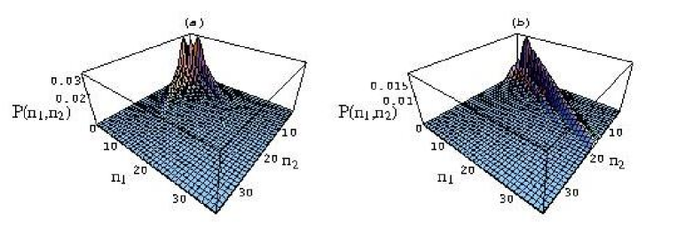
Figure 32: (a) Joint probability $P(n_{1},n_{2})$ of two-mode, two-photon squeezed states ($|\gamma|=0$), for the symmetric choice $\alpha_{1}=\alpha_{2}=1$ of the coherent amplitudes, and with a squeezing parameter $r=1.5$. (b) Joint probability $P(n_{1},n_{2})$ of HEMPSS with lowest order nonlinearities $F(Z)=Z^{2}$ of equal strength $|\gamma|=0.3$. The canonical conditions $\theta_{1}+\theta_{2}-\phi=0$, and $\delta_{1}+\delta_{2}-\phi=\pi$ have been assumed, with assigned values $\delta_{1}=\pi/3$, and $\theta_{1}=-\theta_{2}=\pi/4$. Same values of the squeezing parameter and of the coherent amplitudes as in (a).

Comparing the two cases, we see that the additional parameters associated to the nonlinearity destroy the symmetry possessed by the joint probability in the absence of the nonquadratic interaction. In order to recover symmetric forms of the joint probability $P(n_{1},n_{2})$ for HEMPSS, the various phases must be suitably balanced, as illustrated in Ref. [480]. In general, the many adjustable parameters allow to vary the properties of the joint photon number distribution. In a similar way, we can control and sculpture the mean photon numbers $\langle n_{1}\rangle$ and $\langle n_{2}\rangle$, and the second-order correlation functions, in particular, the cross-correlation function $g^{(2)}_{12}(0)=\langle a_{1}^{{\dagger}}a_{1}a_{2}^{{\dagger}}a_{2}\rangle/\langle a_{1}^{{\dagger}}a_{1}\rangle\langle a_{2}^{{\dagger}}a_{2}\rangle$. In Fig. (33) (a) and (b) we have plotted the mean photon number $\langle n_{1}\rangle$ of the first mode, and the cross-correlation $g^{(2)}_{12}(0)$, as functions of the two heterodyne phases $\theta_{1}$ and $\theta_{2}$, for fixed values of the other parameters.

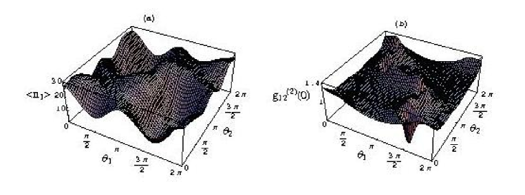
Figure 33: (a) Average number of photons $\langle n_{1}\rangle$ in the original field mode $a_{1}$, as a function of the heterodyne angles $\theta_{1}$, $\theta_{2}$, for a HEMPSS with $\beta_{1}=\beta_{2}=3$, $r=0.5$, $|\gamma|=0.3$, and $\delta_{1}=\pi$. (b) Cross-correlation $g^{(2)}(0)$ as a function of $\theta_{1}$ and $\theta_{2}$, for the same values of the parameters as in (a). In both cases, the imposed canonical constraints read $\theta_{1}+\theta_{2}-\phi=0$ and $\delta_{1}+\delta_{2}-\phi=\pi$.

Once more, one can see that the tuning of the heterodyne phases realizes wild variations of the statistical properties of the HEMPSS. In particular, Fig. (33) (b) shows that both the strong suppression ($g^{(2)}_{12}(0)>0$) and the strong enhancement ($g^{(2)}_{12}(0)<0$) of the anticorrelations between modes $a_{1}$ and $a_{2}$ can be realized as $\theta_{1}$ and $\theta_{2}$ are varied.

6.4 Heterodyne multiphoton squeezed states: diagonalizable Hamiltonians and unitary evolutions

The most elementary Hamiltonian that can be associated to the two-mode nonlinear transformations (388) is the diagonal Hamiltonian of the form

$$H_{2}^{diag}\,=\,b_{1}^{{\dagger}}b_{1}\,+\,b_{2}^{{\dagger}}b_{2}\;.$$ (406)

Inserting Eqs. (388) for the transformed variables in this expression, yields multiphoton Hamiltonians written in terms of the fundamental mode variables $a_{i}$ and $a_{i}^{{\dagger}}$, each one characterized by a specific choice of the nonlinear function $F$. In analogy with the fully degenerate case, in this two-mode context one must look again for interactions that may allow particularly interesting and physically realistic implementations. To this aim, let us consider Hamiltonians associated to nonlinear functions $F$ that are simple, positive powers of their argument: $F(\zeta)=\zeta^{n}$. These Hamiltonians describe a combination of nondegenerate and degenerate multiphoton interaction processes, up to $2n$-th nonlinear order. As usual, we concentrate our attention on the simplest choice of the lowest nonlinearity $F(\zeta)=\zeta^{2}$, describing up to four-photon processes. In this case, the general four-photons Hamiltonian of the form $H_{2}^{diag}$ becomes

$$H_{2G}^{4ph} \,=\, A_{0}+B_{0}(a_{1}^{{\dagger}}a_{1}+a_{2}^{{\dagger}}a_{2})+C_{0}(a_{1}^{{\dagger}2}a_{1}^{2}+a_{2}^{{\dagger}2}a_{2}^{2}+2a_{1}^{{\dagger}}a_{1}a_{2}^{{\dagger}}a_{2})$$ (407)

$$+ [D_{1}a_{1}^{{\dagger}}a_{2}^{{\dagger}}+D_{2}a_{1}^{{\dagger}2}a_{2}+D_{2}^{\prime}a_{1}a_{2}^{{\dagger}2}+D_{3}a_{1}^{{\dagger}3}+D_{3}^{\prime}a_{2}^{{\dagger}3}+D_{4}a_{1}^{{\dagger}2}a_{2}^{{\dagger}2}$$

$$+ D_{5}(a_{1}^{{\dagger}2}a_{1}a_{2}^{{\dagger}}+a_{1}^{{\dagger}}a_{2}^{{\dagger}2}a_{2})+H.c.]\;.$$

This Hamiltonian contains, besides the free harmonic terms, two-mode down conversion processes, degenerate and semi-degenerate three-photon processes, all the Kerr processes, two-mode down conversion processes modulated by the intensities $a_{i}^{{\dagger}}a_{i}$ $\;(i=1,2)$, and semi-degenerate four-photon down conversion processes.
As in the single-mode formalism, it is possible to reduce the number of simultaneously present interactions by suitably tuning the adjustable parameteres appearing in the Hamiltonian. Again, in analogy to the single-mode case, one can even increase the number of available free parameters by generalizing the Hamiltonian $H_{2}^{diag}$ to the form:

$$H_{2}^{su11}\,=\,\sum_{i=1}^{2}\left[\Omega_{i}b_{i}^{{\dagger}}b_{i}\,+\,\xi_{i}b_{i}^{{\dagger}}\,+\,\xi_{i}^{*}b_{i}\right]\,+\,\eta b_{1}^{{\dagger}}b_{2}^{{\dagger}}\,+\,\eta^{*}b_{1}b_{2}\;,$$ (408)

that once more underlies a $SU(1,1)$ symmetry. The freedom in fixing the many adjustable parameters should allow the reduction of such Hamiltonians to the simplest possible forms describing realistically implementable two-mode multiphoton interactions.
Finally, by exploiting the invertible, two-mode nonlinear canonical transformations (388), the $SU(1,1)$ invariance of the Hamiltonian (408), the eigenvalue equations (397), and the completeness relation (401), one can exactly compute the unitary evolution from the initial vacuum state generated by $H_{2}^{su11}$.

6.5 Experimental realizations: possible schemes and perspectives

In this Subsection, we discuss the possible experimental feasibility of multiphoton processes described by the one-mode and two-mode Hamiltonians introduced above, and the corresponding HOMPSS and HEMPSS . As shown in Section 3, the main difficulties in implementing multiphoton processes in nonlinear media are related both to the weakness of the nonlinear susceptibilities, and to the constraints imposed by energy conservation and phase matching. In the same Section we have seen that success in the fabrication of new nonlinear materials, and the exploitation of highly nontrivial effects as coherent population trapping and electromagnetically induced transparency, have led to a sensible enhancement of the third-order $\chi^{(3)}$ nonlinearity, and to the prospect of enhancing the magnitude of higher-order susceptibilities by several orders of magnitude. However, even putting aside this problem, it becomes increasingly difficult to satisfy the energy and phase matching constraints with increasing order of the multiphoton process to be implemented.
In order to show the complexity of practical implementations, we consider now the simple, but relevant, case of collinear multiphoton processes with nonlinear terms of the general form $a_{1}^{{\dagger}}a_{2}^{{\dagger}}\cdots a_{s}^{{\dagger}}a_{s+1}\cdots a_{n}E^{\pm}_{1}\cdots E^{\pm}_{m}$, where the $\{E^{\pm}_{i}\}$ are classical pumps. A collinear process is defined by the condition that the fields associated to all the modes share the same direction of propagation (i.e. the wave vectors are parallel or anti-parallel). We denote by $\omega_{i}$ and $k_{i}$ the frequency and the wave vector associated to the mode $a_{i}$, and by $\Omega_{i}$ and $K_{i}$ the frequency and momentum associated to a classical pump $E_{i}$. We implicitly include in the frequencies $\Omega_{i}$ associated to a classical pump a sign $\pm$ corresponding to a positive or negative frequency choice of the pump itself; moreover, we include in each momentum $K_{i}$ associated to a classical pump a sign which, in a collinear process, discriminates between backward and forward propagation. Energy conservation and phase matching conditions, in this collinear case, read

$$\sum_{i=1}^{s}\omega_{i}\,-\,\sum_{i=s+1}^{n}\omega_{i}\,=\,\sum_{i=1}^{m}\Omega_{i}\;,$$ (409)

$$\sum_{i=1}^{s}k_{i}\,-\,\sum_{i=s+1}^{n}k_{i}\,=\,\sum_{i=1}^{m}K_{i}\;,$$ (410)

Note that the momenta $k_{i}$ and $K_{i}$, apart the sign, coincide, respectively, with $n(\omega_{i})\omega_{i}$ and $n(\Omega_{i})\Omega_{i}$, where $n(\cdot)$ denotes the frequency-dependent refractive index associated to a given frequency. Therefore, the second equation is a nonlinear equation, with the nonlinearity due to phenomenological quantities such as the refractive indices. Therefore, the solution of the problem defined by the set of coupled equations (409) and (410) is highly nontrivial. To try to solve it, one must choose a suitable number of classical pumps, and a convenient medium that allows birefringence (i.e. ordinary and extraordinary refractive indices) or quasi-phase matching (periodic behavior of the refractive index). However, in arbitrary cases, the equations (409) and (410) may not have physically meaningful solutions, and must thus be analyzed case by case in concrete, specific instances. Here then we discuss the possible experimental realization of the effective interaction described by the specific Hamiltonian (379), associated to the single-mode canonical structure.
We consider the collinear processes generated by the lowest possible nonlinearity in a centrosymmetric crystal, namely the one associated to the third-order susceptibility $\chi^{(3)}$, because, in such a material $\chi^{(2n)}=0$ for all $n$. The crystal is illuminated by two highly intense laser pumps, $E_{1}$, of frequency $\omega$ and ordinary polarization, and $E_{2}$, of frequency $3\omega$ and extraordinary polarization. To achieve the phase matching condition, in the following we refer to the discussion of Section 3, in particular to Eq. (111) and to the definition of positive and negative uniaxial crystals. We consider a negative uniaxial crystal, and we exploit the birefringence to compensate the dispersion effect of the frequency-dependent refractive indices $n_{\omega}$. In particular, a suitable choice of the phase matching angle $\theta$ between the propagation vector and the optic axis can lead to the equality $n^{ord}_{\omega}=n^{ext}_{3\omega}(\theta)$, needed to realize the three-photon down conversion processes that we wish to engineer. The combined actions of the two classical pumps on the crystal generate, besides the free linear and harmonic terms, the multiphoton processes described in the following, where $\kappa_{lm}$ will denote the coefficient of the generic interaction term $a^{{\dagger}l}a^{m}$, responsible for the creation of $l$ photons and, correspondingly, the simultaneous annihilation of $m$ photons. As previously remarked, all these processes will be generated only by the third-order $\chi^{(3)}$ susceptibility.
The interaction of the pump at frequency $3\omega$ with the nonlinear crystal generates the three-photon down conversion process $\kappa_{30}E_{2}a^{{\dagger}3}+H.c.\,$, with $\kappa_{30}\propto\chi^{(3)}(3\omega;-\omega,-\omega,-\omega)\,$. Moreover, the first pump at frequency $\omega$ generates the additional four-wave process $\kappa_{21}E_{1}a^{{\dagger}2}a+H.c.\,$, with $\kappa_{21}\propto\chi^{(3)}(\omega;-\omega,-\omega,\omega)\,$. The Kerr term $a^{{\dagger}2}a^{2}$ is obviously generated as well. However, the coupling of this term does not contain contributions due to the intense classical pumps; therefore, it can be neglected in comparison to the other, much stronger interactions. Finally, the third-order nonlinearity generates also the two-photon down conversion process $[\kappa_{20}^{{}^{\prime}}E_{1}^{2}+\kappa_{20}^{{}^{\prime\prime}}E_{1}^{*}E_{2}]a^{{\dagger}2}+H.c.\,$, where $\kappa_{20}^{{}^{\prime}}$ and $\kappa_{20}^{{}^{\prime\prime}}$ are proportional to $\kappa_{21}$ and $\kappa_{30}$, respectively. The contributions associated to the couplings $\kappa_{21}$ and $\kappa_{20}^{{}^{\prime}}$ are due to the self-phase-modulation mechanism, and are automatically phase-matched, while the contribution associated to the coupling $\kappa_{20}^{{}^{\prime\prime}}$ is generated by the simultaneous interaction of the two external pumps with the medium. The total effective interaction Hamiltonian is then finally the experimentally feasible form of the desired reduced three-photon Hamiltonian (379), and, in more detail, it reads

$$H_{exp}^{3ph}\,=\,[\kappa_{20}^{{}^{\prime}}E_{1}^{2}+\kappa_{20}^{{}^{\prime\prime}}E_{1}^{*}E_{2}]a^{{\dagger}2}\,+\,\kappa_{21}E_{1}a^{{\dagger}2}a\,+\,\kappa_{30}E_{2}a^{{\dagger}3}\,+\,H.c.\quad.$$ (411)

In the interaction picture, the coefficients appearing in Eq. (411) are time-independent, and thus Hamiltonian $H_{exp}^{3ph}$ describes the same processes as does Hamiltonian (379). The residual freedom (allowed by the canonical conditions) in fixing the parameters of the theoretical Hamiltonian (379), and the possibility of selecting the desired intensities of the classical pumps in the “experimental” Hamiltonian (411), are then sufficient to assure that the two expressions coincide. As a consequence, at least a particular form of the general single-mode Hamiltonian $H_{1}^{su11}$ of canonical multiphoton quantum optics can be experimentally realized. This fact implies that there exist, at least in principle, physically implementable multiphoton processes that can be associated to nonquadratic Hamiltonian evolutions, exactly determined with the canonical methods described in Subsection 6.2, which generate nonclassical, non Gaussian, single-mode multiphoton squeezed states of the electromagnetic field.

7 Application of multiphoton quantum processes and states to quantum communication and information

7.1 Introduction and general overview

In the last two decades, systems of quantum optics are progressively emerging as an important test ground for the study and the experimental realization of quantum computation protocols and quantum information processes. In this Section, after a very brief resume of some essential concepts of quantum information theory, we discuss the role and possible applications of nonlinear interactions and multiphoton states in this rapidly growing discipline. Clearly, in this short summary, we will only sketch some guidelines into this very extended and complex field of research. The main issues to be discussed here will be the use of multiphoton quantum states as carriers of information, and the manipulation of the latter by the methods of quantum optics.
Mainstream research directions in the theory of quantum communication and information include, among others, quantum cryptography, teleportation, quantum error correction, approximate quantum state cloning, entanglement swapping, and, of course, quantum computation [492, 493, 494, 495, 496, 497, 498, 499, 500, 501, 502]. The growing interest in quantum information and quantum computation arises from the fact that the basic aspects of quantum mechanics, the superposition principle and the Heisenberg uncertainty principle, lead to the existence of non factorizable (nonseparable) dynamics and states, and their associated peculiar quantum correlations. In fact, the nonseparable states of quantum mechanics are endowed with a structure of correlations, that by now goes under the commonplace name of entanglement, allowing, in principle, computational and informational tasks that are believed to be impossible in the realm of classical informatics. This peculiar structure of the correlations in nonseparable quantum states, this entanglement, can thus be regarded as true physical resources for the realization of logical gates, computational protocols, information processes. From the specific point of view of quantum optics, quantum computation and information are becoming very close benchmarks, together with nanotechnology, because, due the fast and constant trend towards the reduction in the energy content of optical signals and the miniaturization of optical components, the consequences of the underlying quantum behaviours begin to emerge in ways that are progressively more pronounced. In particular, as one gets closer and closer to the quantum regime, the direct consequences of the uncertainty principle begin to matter, and the omnipresent fluctuations of the electromagnetic vacuum constitute a source of noise that affects the information carried by optical signals from the initial generation during all its time evolution, and imposes limitations on the fidelity of the transmission. Fortunately, the progresses in nonlinear optics and cavity quantum electrodynamics allow at present several strategies for the control and reduction of vacuum fluctuations and quantum noise in computational and informational processes. This is why quantum optical implementations may turn out to be of paramount importance in the future of quantum information: as already seen, the most common and efficient methods for the reduction of quantum noise are based on squeezed light generation via parametric down conversion, quantum nondemolition measurements, and confinement of electromagnetic fields in cavities. For further discussions and bibliographical sources on noise limitations in optical communication systems, the interested reader may profit of Ref. [503].
We have already mentioned that quantum information science is rooted in two key concepts, respectively the quantum superposition principle and quantum entanglement. Quantum state superpositions allow an enrichment of the information content of the signal field, as they can assume different values at the same time, while the information, through the entanglement effects, becomes a nonlocal property of the whole system. Finally, the requirements of scalability and resilience to decoherence, necessary to achieve efficient quantum computation and secure quantum communication, impose the need for large sets of macroscopic superpositions sharing degrees of multipartite entanglement as large as possible. Consequently, in order to implement efficiently quantum information protocols in a quantum optical setting, it would be of primary importance to devise methods for the engineering of entangled multiphoton superposition states, possibly robust against dissipation and environmental decoherence. Thus motivated, in the following we will review and discuss the theory and the present status of the experimental realizations of these states, and assess their relevance and use in view of efficient implementations of quantum information protocols.

7.2 Qualifying and quantifying entanglement

The entanglement of quantum states of bipartite and multipartite systems is one of the fundamental resources in quantum information. Therefore, in this Subsection we will give a self-contained review on the most relevant measures devised to quantify entanglement in a quantum state, and on the most significant criteria of inseparability.
For bipartite pure quantum states there is a unique measure of entanglement, named entropy of entanglement, defined by the von Neumann entropy of any of the reduced states [504]. Let $\rho_{12}\equiv\rho_{P}$ be a pure state of two parties, its entropy of entanglement $E(\rho_{P})$ is given by

$$E(\rho_{P})=S(\rho_{1})=S(\rho_{2})\,,$$ (412)

where $S(\sigma)=-Tr[\sigma\log_{2}\sigma]$, and $\rho_{i}=Tr_{j\neq i}[\rho_{P}]$ $(i,j=1,2)$. For a system composed of two $N$-level subsystems, the quantity $E$ ranges from zero, corresponding to a product state, to $\log_{2}N$, corresponding to a maximally entangled state. The minimum set of essential properties that should be shared by any bona fide measure of entanglement are the following: it must be positive semi-definite, achieving zero only for separable states; it must be additive; and, finally, it must be conserved under local unitary operations and must be non-increasing on average under local operations and classical communication (LOCC). The entropy of entanglement of pure quantum states satisfies all of the above properties. Under realistic conditions, only partially entangled mixed states can be generated, rather than fully entangled pure states. Unfortunately, in the case of mixed states the von Neumann entropy of the reduced states fails to distinguish classical and quantum correlations and is therefore no longer a good measure of quantum entanglement. Another entropy-based measure for a state $\rho_{12}$ is the von Neumann mutual information [504]:

$$I_{N}(\rho_{1};\rho_{2};\rho_{12})=S(\rho_{1})+S(\rho_{2})-S(\rho_{12})\;.$$ (413)

However, the mutual information $I_{N}$ can increase under local nonunitary operations, therefore it cannot be a good measure of entanglement.
Although the problem of quantifying the amount of entanglement in mixed states is still open, several measures have been proposed in the last years [505, 506, 507, 508, 509]. For a mixed state $\rho_{12}\equiv\rho_{M}$, Bennett et al. have introduced the so called entanglement of formation $E_{F}(\rho_{M})$, defined as the infimum of the entropy of entanglement of the state $\rho_{M}$ computed over all its possible (in general, infinite) pure state decompositions [505].
The same authors have defined another important measure of mixed-state entanglement, the entanglement of distillation $E_{D}(\rho_{M})$, defined as the number of bipartite maximally entangled states (Bell pairs) that can be distilled (purified) from the state $\rho_{M}$ [505]. We recall that the purification or distillation protocol is the procedure of concentrating maximally entangled pure states from partially entangled mixed states by means of local operations and classical communication [510, 511, 512]. Nevertheless, and remarkably, it is not always possible to distill the entanglement of any inseparable states; in fact there exist states, the so called bound entangled states, whose entanglement is not distillable [513, 514].
The entanglement of formation and the entanglement of distillation, although conceptually well defined, are extremely hard to compute due to the infinite dimension of the minimization procedure they involve. It is thus remarkable that the entanglement of formation has been computed exactly in the case of an arbitrary mixed state of two qubits [515], and for an arbitrary mixed symmetric two-mode Gaussian state of continuous variable systems [516].
Vedral et al. have introduced a further measure of entanglement, the relative entropy, which is a suitable generalization of the mutual information Eq. (413) and is defined as [506]:

$$E_{re}(\rho_{12})=\min_{\sigma\in\mathcal{D}}S(\rho_{12}\parallel\sigma)\,,$$ (414)

where $\rho_{12}$ is the state whose entanglement one wishes to compute; $S(\rho_{12}\parallel\sigma)=Tr[\rho_{12}(\ln\rho_{12}-\ln\sigma)]$ is an entropic measure of distance between the two density matrices $\rho_{12}$ and $\sigma$; and $\mathcal{D}$ is the set of the density matrices corresponding to all disentangled states. Extensions of the relative entropy to quantify the entanglement of states of systems composed by more than two subsystems are also possible [506]. From an operational point of view, the entanglement measured by Eq. (414) can be interpreted as the quantity that determines “the least number of measurements needed to distinguish a given state from a disentangled state” [507]. The relative entropy of entanglement $E_{re}$ interpolates between the entanglement of formation $E_{F}$ and the entanglement of distillation $E_{D}$, according to hierarchy $E_{D}\leq E_{re}\leq E_{F}$ [517].
An effectively computable measure of entanglement, the negativity, has been introduced independently by several researchers [509, 518, 519, 520, 521, 522]. This measure is based on the Peres-Horodecki criterion of positivity under partial transposition (PPT criterion) [523, 524]. Let us recall that the partial transposition corresponds to a partial time reversal transformation or to a partial mirror reflection in phase space. By definition, a quantum state of a bipartite system is separable, and we will write it as $\rho_{12}^{(sep)}$, if and only if it can be expressed in the form [525]

$$\rho_{12}^{(sep)}=\sum_{i}p_{i}\,\rho_{i1}\otimes\rho_{i2}\,,\qquad p_{i}\geq 0\,,\qquad\sum_{i}p_{i}=1\;,$$ (415)

that is, as a convex combination of product states of the two subsystems, where $\rho_{i1}$ and $\rho_{i2}$ are, respectively, the normalized states of the first and of the second party. The operation of partial transposition $T_{j}\rho$ ($j=1,2$) on a generic quantum state $\rho$ of a bipartite system with respect to one party is symmetric under the exchange of the two parties. Then, choosing, say, party $j=2$ this operation is defined as follows: $\rho\rightarrow\rho^{T_{2}}$ generates the partially transposed matrix $\rho^{T_{2}}$, whose elements, expressed in an orthonormal basis $|i_{1},j_{2}\rangle$, read:

$$\langle i_{1},j_{2}|\rho^{T_{2}}|k_{1},l_{2}\rangle=\langle i_{1},l_{2}|\rho|k_{1},j_{2}\rangle\;.$$

Let us denote by $\tilde{\rho}$ the partially transposed state $\rho^{T_{2}}$. Then, if the original state is separable, partial transposition must yield again a separable state, i.e.

$$\tilde{\rho}_{12}^{(sep)}\,\equiv\,\left(\rho_{12}^{(sep)}\right)^{T_{2}}\,=\,\sum_{i}p_{i}\,\rho_{i1}\otimes\rho_{i2}^{T_{2}}\;.$$

Hence, for a generic bipartite state $\rho_{12}$ a necessary condition of separability is that the partially transposed matrix $\tilde{\rho}_{12}$ be a bona fide density matrix, i.e. that it be positive semidefinite. This is equivalent to require the nonnegativity of all the eigenvalues of $\tilde{\rho}_{12}$ [523]. Viceversa, the existence of negative eigenvalues of $\tilde{\rho}_{12}$ is a sufficient condition for entanglement. By exploiting this relevant result, a natural measure of entanglement for the state $\rho_{12}$ can be defined as the sum of the moduli of the negative eigenvalues of $\tilde{\rho}_{12}$. This quantity defines the negativity, and is denoted by $\mathcal{N}(\rho_{12})$ [509]:

$$\mathcal{N}(\rho_{12})\,=\,\frac{\parallel\tilde{\rho}_{12}\parallel_{1}-1}{2}\;.$$ (416)

An alternative definition is the logarithmic negativity $E_{\mathcal{N}}(\rho_{12})$ [509]:

$$E_{\mathcal{N}}(\rho_{12})=\log_{2}\parallel\tilde{\rho}_{12}\parallel_{1}\;.$$ (417)

The quantities (416) and (417) are monotone under LOCC and can be easily computed in general, at least numerically.
Let us consider the important instance of two-mode Gaussian states $\rho_{G}$ of continuous variable (CV) systems, for which the PPT criterion is a necessary and sufficient condition for separability, as shown by Simon [526]. These states define the set of two-mode states with Gaussian characteristic functions and quasi-probability distributions, such as the two-mode squeezed thermal states. By defining the vector of quadrature operators $R=(X_{1},\,P_{1},\,X_{2},\,P_{2})$, these states are completely characterized by the first statistical moments $\langle R_{i}\rangle$ and by the covariance matrix $\mathbf{\sigma}$, defined as $\sigma_{ij}=\frac{1}{2}\langle R_{i}R_{j}+R_{j}R_{i}\rangle-\langle R_{i}\rangle\langle R_{j}\rangle$, or in the convenient block-matrix form

$$\mathbf{\sigma}\,=\,\left(\begin{array}[]{cc}\mathbf{A}&\mathbf{C}\\ \mathbf{C}^{T}&\mathbf{B}\end{array}\right)\;,$$ (418)

where $\mathbf{A}$, $\mathbf{B}$, and $\mathbf{C}$ are $2\times 2$ submatrices.
Let us recall that, due to Williamson theorem [527], the covariance matrix of an $n$-mode Gaussian state can always be written as $\mathbf{\sigma}=S^{T}\mathbf{\nu}S$, where $S\in Sp(2n,\mathbb{R})$ is a symplectic transformation, and $\mathbf{\nu}=diag(\nu_{1},\nu_{1},\ldots,\nu_{n},\nu_{n})$ is the covariance matrix of a thermal state written in terms of the symplectic spectrum of $\mathbf{\sigma}$ whose meaning will be clarified below [528]. Here, the elements of the (real) symplectic group $Sp(2n,\mathbb{R})$ are the linear transformations $S$ in phase space with $\det S=1$ that preserve the symplectic form $\Omega$, i.e. such that $S^{T}\Omega S=\Omega$, where

$$\Omega=\bigoplus_{1}^{n}\mathbf{J}\;,\qquad\mathbf{J}=\left(\begin{array}[]{cc}0&1\\ -1&0\end{array}\right)\;,$$ (419)

and $\mathbf{J}$ is the symplectic matrix. By the Stone-von Neumann theorem, symplectic transformations on quasi-probability distributions in phase space correspond to unitary transformations on state vectors in Hilbert space. The quantities $\nu_{i}$ that constitute the symplectic spectrum are the eigenvalues of the matrix $|i\Omega\sigma|$ [528, 529]. In order to compute the negativity (416) and the logarithmic negativity (417) for two-mode Gaussian states, one has to compute the two symplectic eigenvalues $\tilde{\nu}_{\mp}$ (with $\tilde{\nu}_{-}<\tilde{\nu}_{+}$) of the matrix $|i\Omega\tilde{\sigma}|$, where $\tilde{\sigma}$ is the covariance matrix of the partially transposed state $\tilde{\rho}_{G}$. Given the two $Sp(2,\mathbb{R})\oplus Sp(2,\mathbb{R})$ symplectic invariants $\det\mathbf{\sigma}$ and $\tilde{\Delta}(\sigma)=\det\mathbf{A}+\det\mathbf{B}-2\det\mathbf{C}$, the two symplectic eigenvalues $\tilde{\nu}_{\mp}$ read [529, 530]:

$$\tilde{\nu}_{\mp}=\sqrt{\frac{\tilde{\Delta}(\sigma)\mp(\tilde{\Delta}(\sigma)^{2}-4\det\mathbf{\sigma})^{1/2}}{2}}\;.$$ (420)

Finally, it is easy to show that for any two-mode Gaussian state $\rho_{G}$ the negativity is a simple decreasing function of $\tilde{\nu}_{-}$ [530, 531]:

$$\parallel\tilde{\rho}_{G}\parallel_{\,{}_{1}}\,=\,\frac{1}{\tilde{\nu}_{-}}\;,$$ (421)

$$\mathcal{N}(\rho_{G})=\max\left[0,\,\frac{1-\tilde{\nu}_{-}}{2\tilde{\nu}_{-}}\right]\;,$$ (422)

$$E_{\mathcal{N}}(\rho_{G})=\max[0,\,-\log_{2}\tilde{\nu}_{-}]\;.$$ (423)

As already mentioned before, for two-mode symmetric Gaussian states (i.e. for two-mode Gaussian states with $\det\mathbf{A}=\det\mathbf{B}$) the entanglement of formation $E_{F}(\rho_{G})$ can be computed as well [516], and coincides in this case with the logarithmic negativity but for irrelevant scale factors. It is likely that this equivalence breaks down in more general instances of mixed Gaussian states. For instance, it has been recently shown that a rigorous bound for the true entanglement of formation, the so-called Gaussian entanglement of formation (i.e. the entanglement of formation computed only on pure Gaussian state convex decompositions) [532] does not coincide in general with the logarithmic negativity for particular classes of mixed nonsymmetric two-mode Gaussian states [533]. Moreover, for these states the two measures induce different orderings, in the sense that, taken a reference state, another state will be more or less entangled than the reference state depending whether one chooses the Gaussian entanglement of formation or the logarithmic negativity to quantify entanglement [533]. Generalizations are straightforward for particular classes of fully symmetric and bisymmetric multimode Gaussian states. In these instances the negativities are again amenable to a complete analytic computation, and the entanglement quantified by them possesses interesting properties of scaling and unitary localization [534, 535]. Finally, in order to analyze entanglement in a multipartite system, the different bipartite splittings of the whole system can be considered [536]. This procedure can be used to define multipartite negativities, as shown in Ref. [509].

Besides facing the hard task of quantifying the exact amount of entanglement in a given quantum state, it is in principle important, and often interesting for practical purposes, to establish its inseparability properties. To this end, it is necessary to look for reliable (in)separability criteria, and several ones have been proposed for bipartite states [523, 524, 526, 537, 538, 539, 540, 541, 542, 543, 544, 545, 546, 547, 548]. Such criteria often take the form of inequalities and usually provide sufficient conditions for inseparability. However, in the case of two-mode Gaussian states and of multimode Gaussian states of $1\times N$ bipartitions, it is possible to establish criteria that are necessary and sufficient for inseparability. As already mentioned, the continuous-variable version of the PPT criterion is a necessary and sufficient condition for separability of two-mode Gaussian states, as first proved by Simon [526], and of multimode Gaussian states of $1\times N$ bipartitions, as shown by Werner and Wolf [549]. A further criterion, due to Duan et al. [539], based on suitably scaled Einstein-Podolski-Rosen (EPR) observables, turns out to be necessary of sufficient for the separability of two-mode Gaussian states.
On the other hand, as seen in Sections 4 and 5, the most recent theoretical and experimental efforts are concerned with the engineering of highly nonclassical, non-Gaussian states of the radiation field, in order to enhance either the entanglement [550, 551], or other useful properties as the quantum robustness against decoherence [552]. Furthermore, even if at present Gaussian states continue to play a central role in quantum optics and quantum information, it has been shown rigorously that some fundamental physical properties, such as the entanglement and the distillable secret key rate, are minimized by Gaussian states [553]. In a sense, this result is not surprising. Gaussian states are the most semiclassical among quantum states, and entanglement is a genuine quantum property that essentially originates from the superposition principle. The inseparability criteria that have been introduced so far provide only sufficient conditions on the inseparability of non-Gaussian states. Therefore, they can fail in detecting quantum correlations for some sets of genuinely entangled states [546].
Before reviewing some of the most significant inseparability criteria, we describe a sufficiently general approach to their construction for bipartite systems of continuous variables. A natural starting point to search for a necessary condition for separability (sufficient condition for entanglement) is the general definition by Werner of separable states, Eq. (415). One then proceeds to select a suitable operatorial function $f$ of the annihilation and creation operators associated to the two subsystems, considers its mean values in a generic, separable state written in the Werner form Eq. (415), and derives an inequality constraint. Let us consider first the two EPR-like operators of the form

$$U=|a|X_{1}+\frac{1}{a}X_{2}\,,\quad\quad V=|a|P_{1}-\frac{1}{a}P_{2}\;,$$ (424)

where $X_{j}$ and $P_{j}$ $(j=1,2)$ are the position and momentum operators corresponding to the mode $j$, and $a$ is an arbitrary real number. Applying the Cauchy-Schwartz inequality to the total variance $\langle(\Delta U)^{2}\rangle_{\rho}+\langle(\Delta V)^{2}\rangle_{\rho}$, it is easy to show that for any separable quantum state $\rho$ the following inequality must hold

$$\Delta_{EPR}(a)=\langle(\Delta U)^{2}\rangle_{\rho}+\langle(\Delta V)^{2}\rangle_{\rho}-a^{2}-\frac{1}{a^{2}}\geq 0\;,$$ (425)

for any choice of the constant $a$ [539]. As an immediate consequence, if at least a value of $a$ exists such that the inequality (425) is violated, i.e. $\Delta_{EPR}(a)<0$, then $\rho$ is an entangled state. This sufficient condition for inseparability is precisely the criterion formulated by Duan et al. [539]. The criterion is optimized by minimizing $\Delta_{EPR}(a)$ with respect to $a$, while keeping the other variables fixed.
As a second example, let us now consider the criterion due to Simon to obtain a sufficient condition for inseparability in terms of the second order statistical moments of the position and momentum operators [526]. Simon defines the operatorial function

$$\hat{f}\,=\,c_{1}X_{1}+c_{2}P_{1}+c_{3}X_{2}+c_{4}P_{2}\;,$$

and observes that the Heisenberg uncertainty principle is equivalent to the statement

$$\langle\hat{f}^{{\dagger}}\hat{f}\rangle_{\rho}\,=\,Tr[\rho\hat{f}^{{\dagger}}\hat{f}]\,\geq\,0\;.$$

Finally, by applying the PPT requirement (a separable density operator $\rho$ must transform into a non-negative, bona fide density operator $\tilde{\rho}$ under partial transposition), Simon obtains the following necessary condition for separability:

$$Tr[\tilde{\rho}\hat{f}^{{\dagger}}\hat{f}]\,\geq\,0\;.$$ (426)

This condition, in terms of the matrices defined in Eq. (418), reads

$$\det\mathbf{A}\det\mathbf{B}+\left(\frac{1}{4}-|\det\mathbf{C}|\right)^{2}-Tr[\mathbf{AJCJBJC^{T}J}]$$

$$-\frac{1}{4}(\det\mathbf{A}+\det\mathbf{B})\,\geq\,0\;,$$ (427)

where $\mathbf{J}$ is the $2\times 2$ symplectic matrix defined in Eq. (419). Let us recall again that one can easily show that for all two-mode Gaussian states the Duan and the Simon criteria are necessary and sufficient for separability, and thus coincide. Moreover, the Simon criterion given by Eq. (426) or (427) reduces to a simple inequality for the lowest symplectic eigenvalue: $\tilde{\nu}_{-}\geq 1$; or, equivalently, for the covariance matrix: $\tilde{\Delta}(\mathbf{\sigma})\leq\det\mathbf{\sigma}+1$ (with $\mathbf{\sigma}$ given by Eq. (418)).
Other interesting criteria include the so-called “product” condition introduced by Giovannetti et al. [541]. Through a method similar to that of Ref. [539], thes authors have found a more general inequality condition, containing as a special case Eq. (425). Man’ko et al. have proposed a generalization of the PPT criterion based on partial transposition by introducing a scaled partial transposition [544]. The associated criterion of positivity under scaled partial transposition (PSPT) might be particularly suitable for the detection of multipartite entanglement.
The EPR- and PPT-type criteria discussed above, i.e. the EPR and PPT criteria suitably adapted to the case of Gaussian states, naturally involve only second order statistical moments of the quadratures. Moving to analyze non Gaussian states, criteria limited to second order moments do not detect entanglement efficiently, and inclusion of higher order moments is needed. Inspired by this motivation, Agarwal and Biswas have proposed new criteria based on inequalities involving higher order correlations [545]. In particular, these authors have combined the method of partial transposition and the uncertainty relations for the Schwinger realizations of the $SU(2)$ and $SU(1,1)$ algebras on generic states. In a two-mode system, the realization of the $SU(1,1)$ algebra, provided by the operators $K_{x}=2^{-1}(a_{1}^{{\dagger}}a_{2}^{{\dagger}}+a_{1}a_{2})$, $K_{y}=(2i)^{-1}(a_{1}^{{\dagger}}a_{2}^{{\dagger}}-a_{1}a_{2})$, $K_{z}=2^{-1}(a_{1}^{{\dagger}}a_{1}+a_{2}^{{\dagger}}a_{2}+1)$; leads to an uncertainty relation that reads:

$$\langle(\Delta K_{x})^{2}\rangle_{\rho}\langle(\Delta K_{y})^{2}\rangle_{\rho}\,\geq\,\frac{1}{4}|\langle K_{z}\rangle_{\rho}|^{2}\;.$$

The PPT prescription under partial transposition, e.g. $\Leftrightarrow$ $a_{2}\leftrightarrow a_{2}^{{\dagger}}$, introduced in the above inequality yields a necessary condition of separability in terms of fourth order statistical moments. In Ref. [545] this approach has been successfully tested on the two-mode non-Gaussian state described by the wave function

$$\psi(x_{1},x_{2})\,=\,(2/\pi)^{1/2}(\gamma_{1}x_{1}+\gamma_{2}x_{2})\exp\{-(x_{1}^{2}+x_{2}^{2})/2\}\;,$$

with $|\gamma_{1}|^{2}+|\gamma_{2}|^{2}=1$. This state is always entangled for all values of $\gamma_{1}$ and $\gamma_{2}$, as can be seen as well by direct application of PPT to the associated density matrix. However, according to the criteria based on second order moments, like the ones by Duan et al and by Giovannetti et al, this state appears to be always separable. The inequality based on fourth order moments is instead sufficient to detect inseparability over the whole range of values of $\gamma_{1}$ and $\gamma_{2}$. Clearly, as already suggested by Agarwal and Biswas, it is desirable to develop criteria based on hierarchies of statistical moments of arbitrary order. Progress along this program has been achieved first by Hillery and Zubairy [546], and later, in much greater generality by Shchukin and Vogel [547]. In Ref. [546], Hillery and Zubairy have considered moments of arbitrary order of the form $|\langle a_{1}^{k}a_{2}^{h}\rangle_{\rho}|$ or of the form $|\langle a_{1}^{k}a_{2}^{{\dagger}h}\rangle_{\rho}|$. Then, starting for instance from the first form, one can prove that a necessary condition for the separability of a generic two-mode quantum state is the validity of all the infinite inequalities

$$\Delta_{kh}\,=\,\langle a_{1}^{{\dagger}k}a_{1}^{k}\rangle\langle a_{2}^{{\dagger}h}a_{2}^{h}\rangle-|\langle a_{1}^{k}a_{2}^{h}\rangle|^{2}\geq 0\;,$$ (428)

where $k$ and $h$ are two arbitrary positive integers. Similar relations cab be obtained by starting from the second form. Obviously, the violation of any one of these infinite inequalities is then a sufficient condition for inseparability. It is important to notice that the moments involved in the set of inequalities derived by Hillery and Zubairy do not coincide with the moments involved in the inequalities derived by Agarwal and Biswas when considering the fourth order. However a further generalization containing all the cases previously discussed has been recently introduced by Shchukin and Vogel using an elegant and unifying approach [547]. These authors succeed to express the PPT criterion for two-mode states of continuous variable systems through an infinite hierarchy of inequalities involving all moments of arbitrary order. They consider Eq. (426), with $\hat{f}$ given by

$$\hat{f}\,=\,\sum_{n,m,k,l=0}^{\infty}c_{nmkl}\,a_{1}^{{\dagger}n}a_{1}^{m}a_{2}^{{\dagger}k}a_{2}^{l}\;,$$ (429)

and prove that the PPT separability condition is equivalent to imposing the nonnegativity of an infinite hierarchy of suitably chosen determinants [547]

$$D_{N}\,=\,\left|\begin{array}[]{cccccc}1&\langle a_{1}\rangle&\langle a_{1}^{{\dagger}}\rangle&\langle a_{2}^{{\dagger}}\rangle&\langle a_{2}\rangle&\cdots\\ \langle a_{1}^{{\dagger}}\rangle&\langle a_{1}^{{\dagger}}a_{1}\rangle&\langle a_{1}^{{\dagger}2}\rangle&\langle a_{1}^{{\dagger}}a_{2}^{{\dagger}}\rangle&\langle a_{1}^{{\dagger}}a_{2}\rangle&\cdots\\ \langle a_{1}\rangle&\langle a_{1}^{2}\rangle&\langle a_{1}a_{1}^{{\dagger}}\rangle&\langle a_{1}a_{2}^{{\dagger}}\rangle&\langle a_{1}a_{2}\rangle&\cdots\\ \langle a_{2}\rangle&\langle a_{1}a_{2}\rangle&\langle a_{1}^{{\dagger}}a_{2}\rangle&\langle a_{2}^{{\dagger}}a_{2}\rangle&\langle a_{1}^{2}\rangle&\cdots\\ \langle a_{2}^{{\dagger}}\rangle&\langle a_{1}a_{2}^{{\dagger}}\rangle&\langle a_{1}^{{\dagger}}a_{2}^{{\dagger}}\rangle&\langle a_{2}^{{\dagger}2}\rangle&\langle a_{2}a_{2}^{{\dagger}}\rangle&\cdots\\ \cdots&\cdots&\cdots&\cdots&\cdots&\cdots\\ \end{array}\right|\;,$$ (430)

i.e. $D_{N}\geq 0$ $\forall N$. Viceversa, if there exists at least one negative determinant, i.e. if

$$\exists N\;:\qquad D_{N}\,<\,0\;,$$

this is a sufficient condition for inseparability of the state [547].

7.3 Engineering and applications of multiphoton entangled states: theoretical proposals and experimental realizations

A very nice feature of quantum optics is that it is flexible and versatile enough to provide the necessary tools for quantum information based either on discrete or on continuous variables. Discrete-variable quantum information deals with elaborating, storing, manipulating, and transmitting information encoded in quantum states with a discrete spectrum of eigenvalues, and thus belonging to finite-dimensional Hilbert spaces. In the simplest instance of two-dimensional Hilbert spaces, the elementary units of information are then two-state (two-level) systems, universally known as qubits in the quantum-informatic jargon. All the possible superposition states of a two-level system can be expressed in terms of linear combinations of two-dimensional orthonormal states defining the standard computational basis. In a quantum optical setting, these basis states can be realized as the two orthonormal eigenstates of the photon polarization observable, respectively, the horizontally $(H)$ and vertically $(V)$ polarized one-photon states

$$|H\rangle\,=\,\left(\begin{array}[]{c}1\\ 0\\ \end{array}\right)\;,\quad\quad\quad|V\rangle\,=\,\left(\begin{array}[]{c}0\\ 1\\ \end{array}\right)\;.$$ (431)

On the other hand, to the electromagnetic field are associated other physical objects, such as the phase and amplitude quadratures (”position” and ”momentum”), that are continuous variables, i.e. generalized observables with a continuous spectrum of eigenvalues. Quantum information based on continuous variables is then characterized by the fact that the information is carried by quantum states belonging to infinite-dimensional Hilbert spaces. Thus, quantum optics enables in principle to realize the encoding of quantum information either with polarization qubits or with continuous quadratures. In fact, it allows much more. Namely, all intermediate possibilities for encoding information can be realized by exploiting superpositions of a finite number of macroscopically distinguishable states [554, 555], so that, in a quantum optical framework, a generic superposition state of a qubit can be constructed, e. g., as the superposition of two distinguishable continuous variables states, for example the two coherent states of $\pi$-opposite phase $|\alpha\rangle$ and $|-\alpha\rangle$. Then, the generic continuous-variable qubit state in this case reads

$$|\psi\rangle\,=\,\xi_{1}|\alpha\rangle+\xi_{2}|-\alpha\rangle\;,$$ (432)

where the complex coefficients $\xi_{i}$ satisfy the normalization condition $|\xi_{1}|^{2}+|\xi_{2}|^{2}+2Re[\xi_{1}^{*}\xi_{2}\langle\alpha|-\alpha\rangle]=1$. For large values of $|\alpha|^{2}$ the two states $|\pm\alpha\rangle$ will be approximately orthogonal, and thus they will realistically approximate the vectors of the computational basis.
We will now turn to discuss both discrete-variable and continuous-variable schemes of quantum computation and information. We begin by introducing the general concept of quantum computer, probably the most fascinating object of theoretical investigation in the field of quantum information. In principle, it is expected that a quantum computer will allow to solve problems exponentially faster than any classical computer [556, 557, 558, 559, 560, 561]. A simple prescription for the construction of such a machine was given by Deutsch [562]: it is a set of $n$ qubits on which unitary operations or quantum logic gates can be applied. It is well known [492] that a unitary transformation (one-bit gate) and a two-bit conditional quantum phase gate are sufficient to build a universal quantum computer. The one-bit gate is the so-called universal quantum gate which by its repeated use can generate all unitary transformations of the qubits, and it reads

$$U_{\theta,\phi}\,=\,\left(\begin{array}[]{cc}\cos\theta&-ie^{-i\phi}\sin\theta\\ -ie^{i\phi}\sin\theta&\cos\theta\\ \end{array}\right)\;.$$ (433)

The transformation for a two-bit phase gate is instead given by

$$Q_{\phi}^{(2)}|\xi,\eta\rangle\,\equiv\,e^{i\phi\delta_{\xi,V}\delta_{\eta,V}}|\xi,\eta\rangle\;,$$ (434)

where $|\xi,\eta\rangle=|\xi\rangle|\eta\rangle$ and $\xi,\eta=H,V$. It is to be noted that the set of the linear unitary transformations is not sufficient to implement the universal quantum computation; this implies that nonlinear transformations are needed too. From this point of view, several schemes have been proposed to realize qubit-based quantum computation [563, 564, 565]. In particular, Knill, Laflamme, and Milburn have demonstrated that, in principle, robust and efficient quantum computing is possible by combining linear optical elements with photodetectors inducing nonlinear transformations [564]. On the other hand, resonantly enhanced nonlinearities can offer some advantages in the implementation of quantum computing protocols. Let us consider some examples [113, 117] which refer to recent proposals for the realization of phase gates. The transformation (434) can be realized by exploiting an enhanced $\chi^{(3)}$ cross-Kerr interaction [113], whose corresponding unitary operator reads $Q_{\phi}^{(2)}=e^{i\phi a_{V}^{{\dagger}}a_{V}b_{V}^{{\dagger}}b_{V}}$. The interaction $H_{5}=\kappa^{(5)}a_{V}^{{\dagger}}a_{V}b_{V}^{{\dagger}}b_{V}c_{V}^{{\dagger}}c_{V}$, realizable in an enhanced $\chi^{(5)}$ medium [117], can be used for the implementation of Grover’s quantum search algorithm [566]. A weak cross-Kerr nonlinearity has also been used to construct a CNOT gate based on a quantum nondemolition measurement scheme [567].
All the examples that we have just cited, refer to schemes involving multiphoton processes in nonlinear media for the realization of information protocols with discrete variables. However, as shown by Lloyd and Braunstein [568, 569, 570], a universal quantum computer can be in principle realized over continuous variables as well, although limited to the classes of transformations that are polynomial in those variables. Considering as continuous variables the quadrature amplitudes $\{X,P\}$ of the electromagnetic field, these transformations might be implemented by means of simple optical devices such as beam splitters, phase shifters, squeezers, and Kerr-effect fibers [570]. Let us consider the application of a sequence of Hamiltonians $H_{i}$, $H_{j}$, $-H_{i}$, $-H_{j}$, each for a time $\delta t\rightarrow 0$; in this limit the following relation holds

$$e^{iH_{i}\delta t}e^{iH_{j}\delta t}e^{-iH_{i}\delta t}e^{-iH_{j}\delta t}\,=\,e^{(H_{i}H_{j}-H_{j}H_{i})\delta t^{2}}\,+\,\mathcal{O}(\delta t^{3})\;.$$ (435)

Relation (435) means that the application of the sequence of Hamiltonians is equivalent to the application of the Hamiltonian $i[H_{i},H_{j}]$ for a time $\delta t^{2}$. In general, starting from a set of Hamiltonians $\{\pm H_{i}\}$, any Hamiltonian of the form $\pm i[H_{i},H_{j}]$, $\pm[H_{i},[H_{j},H_{k}]]$, etc. can be constructed [570]. That is, one can construct the Hamiltonians in the algebra generated from the original set of operators by repeated commutations. If one chooses as original set the operators $X$, $P$, $H_{0}=X^{2}+P^{2}$, and $S=(XP+PX)/2$, corresponding to translations, phase shifts, and squeezers, one can construct any Hamiltonian quadratic in $X$ and $P$. Therefore one- and two-photon passive and active optical transformations are enough to simulate any quadratic Hamiltonian associated to second-order (two-photon) processes. In order to obtain Hamiltonians that are arbitrary-order self-adjoint polynomials of $X$ and $P$, it is instead necessary the exploitation of nonlinear, nonquadratic processes like the Kerr interaction $H^{2}=(X^{2}+P^{2})^{2}$. Alternatively, as for the discrete variable case, the photon number measurement can be used to induce a nonlinear transformation [571]. For instance, by exploiting squeezing, phase-space displacement, and photon counting, it is possible to generate the so-called ”cubic-phase state” [571] defined as

$$|\gamma\rangle\,=\,\int dxe^{i\gamma x^{3}}|x\rangle\;.$$ (436)

One can easily see that these cubic phase states coincide with the homodyne multiphoton squeezed states (HOMPSS) [479] discussed in Section 6, in the case of lowest quadratic nonlinearity $F(x)=x^{2}$, and can thus be realized by purely Hamiltonian, unitary evolutions, albeit nonlinear.
The realization of quantum gates can be also implemented by means of teleportation protocols. Quantum teleportation has been originally proposed by Bennett et al. [572] for systems of discrete variables, and successively extended by Vaidman [573] and by Braunstein and Kimble [574] to continuous variables. It consists in the transmission of unknown quantum states between distant users exploiting shared entangled states (resources), and with the assistance of classical communication. Quantum teleportation has been experimentally demonstrated by Bouwmeester et al. [575] and Boschi et al. [576] for the discrete variable case, and by Furusawa et al. [577, 578] in the case of continuous variables. These are important results per se and from the point of view of quantum computing as well, because it has been shown that exploiting quantum teleportation reduces the necessary resources for universal quantum computation [579]. Actually, single-qubit operations, Bell-basis measurements and entangled states as the three-photon Greenberger-Horne-Zeilinger (GHZ) states [580] result to be sufficient for the realization of a universal quantum computer [579]. However, the fundamental tools for the effective realization of teleportation remain bipartite entangled states like the so-called Bell states and devices for Bell-state measurements. Let us first consider the discrete variable instance. The four two-photon maximally polarization-entangled Bell states,

$$|\phi_{\pm}\rangle\,=\,\frac{1}{\sqrt{2}}(|VV\rangle\pm|HH\rangle)\;,\qquad|\psi_{\pm}\rangle\,=\,\frac{1}{\sqrt{2}}(|VH\rangle\pm|HV\rangle)\;,$$ (437)

can be experimentally generated by means of type-II parametric down conversion, as reported by Kwiat et al. [581]. The notation, assumed in Eq. (437) and in the following relations for the discrete variables polarization states, refers to the general definition of the $N$-mode, $N$-photon state $|p_{1}\,p_{2}\,\ldots\,p_{N}\rangle\equiv\bigotimes_{k=1}^{N}|p_{k}\rangle$, in which each mode $k$ is populated by exactly one photon having polarization $p_{k}=H,V$. The possibility to produce such states in nonlinear photonic crystals has been investigated as well [582]. Very recently, the generation of Bell states has been obtained experimentally by Li et al. [583] in an optical fiber in the $1550\;nm$ band of telecommunications. As a complete Bell measurement is very difficult to achieve by means of linear optics [584, 585], schemes for the discrimination of the Bell states, based on nonlinear effects as resonant atomic interactions [586] and Kerr interactions [587, 588], have been proposed.
On the other hand, moving to a continuous variable setting, the Bell measurement can be easily performed by homodyne detection, but it is difficult to generate states with large quadrature entanglement. The continuous variable state $|\Psi_{EPR-B}\rangle$ containing the necessary correlations for teleportation can be obtained by the Einstein-Podolsky-Rosen (EPR) state [490] (already introduced, in a different form, in Section 6), defined as the simultaneous eigenstate of the two commuting observables, total momentum and relative position, of a two-mode radiation field. Let us consider the nondegenerate parametric amplifier $H_{PA}=ir(a_{1}^{{\dagger}}a_{2}^{{\dagger}}-a_{1}a_{2})$; the solution of the Heisenberg equations for the field modes yield the squeezed joint quadratures

$$X_{1}(t)-X_{2}(t)=(X_{1}-X_{2})e^{-rt}\;,\quad P_{1}(t)+P_{2}(t)=(P_{1}+P_{2})e^{-rt}\;.$$ (438)

In the limit $rt\rightarrow\infty$ in which squeezing becomes infinite, or, equivalently, the waiting time becomes very large, these operators commute and admit the common eigenstate

$$|\Psi_{EPR-B}\rangle\;=\;\frac{1}{\sqrt{2\pi}}\int dx|x\rangle_{1}|x\rangle_{2}\;.$$ (439)

These two limits are unrealistic for concrete applications. In a recent paper, van Enk has proposed a scheme that would allow in principle to produce, in arbitrarily short time, an arbitrarily large amount of entanglement in a bipartite system [589]. The scheme is based on the following simple two-step interaction: in the first step one induces the unitary evolution of an initial coherent state in a Kerr medium, and subsequently, in the second step, the output state generated in the first step is feeded to a $50-50$ beam splitter. The final state $|\Psi_{ent}(\tau)\rangle$ is entangled and reads

$$|\Psi_{ent}(\tau)\rangle\,=\,U_{K,BS}|\alpha\rangle_{a}|0\rangle_{b}\,=$$

$$\exp\left\{\frac{\pi}{4}(a^{{\dagger}}b-b^{{\dagger}}a)\right\}\,\exp\{-i\tau a^{{\dagger}2}a^{2}\}|\alpha\rangle_{a}|0\rangle_{b}\;,$$ (440)

where $\tau$ is the dimensionless time. Fixing $\tau\equiv\tau_{m}=\pi/m$, the final state $|\Psi_{ent}(\tau_{m})\rangle$ is a superposition of $m$ two-mode coherent states of the form

$$|\Psi_{ent}(\tau_{m})\rangle\,=$$

$$\left\{\begin{array}[]{cc}\sum_{q=0}^{m-1}f_{q}^{(o)}|\alpha e^{-\frac{2\pi iq}{m}}/\sqrt{2}\rangle|\alpha e^{-\frac{2\pi iq}{m}}/\sqrt{2}\rangle&\qquad m\quad odd\;,\\ &\\ \sum_{q=0}^{m-1}f_{q}^{(e)}|\alpha e^{\frac{i\pi}{m}}e^{-\frac{2\pi iq}{m}}/\sqrt{2}\rangle|\alpha e^{\frac{i\pi}{m}}e^{-\frac{2\pi iq}{m}}/\sqrt{2}\rangle&\qquad m\quad even\;,\end{array}\right.$$ (444)

where the coefficients $f_{q}^{(o)}$ and $f_{q}^{(e)}$ coincide with those of Eq. (188). The two-mode states (444) are entangled with entanglement $E(\tau_{m})\simeq\log_{2}m$ ebits; thus the entanglement increases with increasing $m$ or, equivalently, with decreasing interaction time, leading to an arbitrarily large entanglement in arbitrarily short time. Note that, as mentioned in Section 4, a similar scheme, and the states (444), have been proposed to produce macroscopic superposition states in a short interaction time in the presence of small Kerr nonlinearity [279].
Continuous variable entanglement has been experimentally observed in an optical fiber [590] and in the interaction between a linearly polarized coherent field and cold cesium atoms in a cavity [591].
An exhaustive investigation of continuous variable entanglement of two-mode Gaussian states has been performed by Laurat et al. [592], who, after reviewing the general framework for the characterization and quantification of entanglement, have experimentally produced two-mode squeezed states through parametric amplification in a type-II OPO, and have showed how to manipulate such states to maximize the entanglement. The experimental setup realized in Ref. [592] is similar to that of the seminal work by Ou et al. [593]; a simplified scheme of the setup is depicted in Fig. (34).

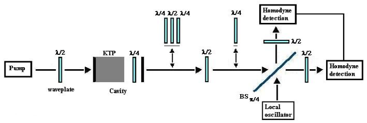
Figure 34: Experimental setup for the production of two-mode squeezed states, and for the characterization and manipulation of their entanglement. A continuous-wave frequency-doubled $Nd:YAG$ laser pumps a type-II OPO ($KTP$ crystal) with a (quarter) $\lambda/4$ waveplate inserted inside a cavity. By suitably inserting the quarter and half waveplates, the covariance matrix of the two-mode Gaussian state can be reconstructed, and the entanglement can be optimized.

The two-mode squeezed state is produced by a frequency-degenerate type-II OPO below threshold; the insertion of a $\lambda/4$ birefringent plate inside the optical cavity allows to produce symmetric Gaussian states, although not in standard form (for the definition of a standard form of a covariance matrix see e.g. Refs. [539, 526]). Laurat et al. show how to theoretically compute and experimentally determine the elements of the matrix (418) through a simultaneous double homodyne detection, and how to optimize the entanglement by using a phase shifter [592]. An improvement of the above experiment has been recently proposed by D’Auria et al. [594]. The improvement amounts to exploiting only one homodyne detection, with the consequent repeated measurements of single-mode quadratures.
In order to implement quantum teleportation by means of linear optics and squeezed light, multipartite entanglement has been exploited by van Loock and Braunstein [595]. They have shown that a $N$-partite, multiphoton entangled state can be generated from $N$ squeezed field modes that are then combined in a suitable way by $N-1$ beam splitters, and that quantum teleportation between two of the $N$ parties is possible with the assistance of the other $N-2$. This quantum teleportation network has been recently demonstrated experimentally for $N=3$ modes [596]. Moreover, it has been shown that the success of a $N$-user continuous variable teleportation network, quantified by the maximal achievable fidelity between the input and the teleported state, is qualitatively and quantitatively equivalent to the presence of genuine multipartite quadrature entanglement in the shared resource states [597]. More generally, multipartite entanglement, either of continuous or of discrete variables, represents a powerful resource to enlarge the field of applications and possible implementations of quantum information protocols, and its study presents very interesting aspects for the understanding of the foundations of quantum theory [495].
Let us now consider some examples of multipartite entangled states and methods for their generation in the quantum optical domain. The most representative multipartite polarization-entangled (discrete variable) states are the $N$-photon GHZ states [580]

$$|{\rm GHZ}_{N}\rangle\,=\,\frac{1}{\sqrt{2}}\left(|\underbrace{VV\ldots V}_{N}\rangle\,+\,|\underbrace{HH\ldots H}_{N}\rangle\right)\;,$$ (445)

and the $N$-photon $W$ states [598]

$$|W_{N}\rangle\,=\,\frac{1}{\sqrt{N}}\left(|\underbrace{H\ldots HV}_{N}\rangle\,+\,|\underbrace{H\ldots HVH}_{N}\rangle\,+\,\ldots\,+\,|\underbrace{VH\ldots H}_{N}\rangle\right)\;.$$ (446)

The GHZ and $W$ states are inequivalent as they cannot be converted into each other under stochastic local operations and classical communications, and therefore differ greatly in their entanglement properties [598, 599]. The GHZ state possesses maximal $N$-partite entanglement, i.e. it violates Bell inequalities maximally; but its entanglement is fragile, because if one or more parties are lost due, for instance, to decoherence, then the entanglement is destroyed. The $W$ state instead possesses less $N$-partite entanglement but it is more robust against the loss of one or more parties, in the sense that each pair of qubits in the reduced state has maximal possible bipartite entanglement. Several successful experiments have been reported on the generation of multiphoton entangled states, in particular the three-, four-, and five-photon GHZ states, and the three-photon $W$ state [600, 601, 602, 603, 604]. Furthermore, many schemes have been proposed for the generation of the four-photon $W$ state and of other four-photon entangled states [605, 606, 607, 608, 609, 610]. We want also to mention the recent observation [611] of the four-photon entangled state

$$|\Psi^{(4)}\rangle= \frac{1}{\sqrt{3}}[|HHVV\rangle+|VVHH\rangle$$ (447)

$$-\frac{1}{2}(|HVHV\rangle+|VHVH\rangle\pm|HVVH\rangle\pm|VHHV\rangle)]\,,$$

which can be expressed as a superposition of a four-photon GHZ state and of a product of two Bell states. The state $|\Psi^{(4)}\rangle$ can be generated directly by a second order parametric down conversion process [608]. In fact, let us consider the multiple emission events in type II parametric down conversion during a single pump pulse, that is

$$\exp\{-i\kappa(a_{V}^{{\dagger}}b_{H}^{{\dagger}}+a_{H}^{{\dagger}}b_{V}^{{\dagger}})\}|0\rangle\;.$$ (448)

The second order term of the exponential expansion corresponds to four-photon effects, and is proportional to

$$(a_{V}^{{\dagger}}b_{H}^{{\dagger}}+a_{H}^{{\dagger}}b_{V}^{{\dagger}})^{2}|0\rangle=$$

$$|2H_{a},2V_{b}\rangle+|2V_{a},2H_{b}\rangle+|1H_{a},1V_{a},1H_{b},1V_{b}\rangle\,.$$ (449)

If this state enters two nonpolarizing beam splitters, the output state $|\Psi^{(4)}\rangle$ can be obtained [608]. Because it is relatively easy to generate, and shows interesting correlation properties, this four-photon state has been proposed as a candidate for the implementation of several communication schemes [611]. A similar four-photon polarization-entangled state, belonging to the class of so-called cluster states [612], that reads

$$|\Phi_{cluster}\rangle\,=\,\frac{1}{2}\left(|HHHH\rangle+|HHVV\rangle+|VVHH\rangle-|VVVV\rangle\right)\;,$$ (450)

has been recently realized experimentally, and exploited for the demonstration of the Grover algorithm [566] on a $4$-photon quantum computer [613]. Other kinds of four-photon entangled states can be obtained from type I down conversion in a cascaded two-crystal geometry [609, 610], see Fig. (14). In the case of collinear nondegenerate down conversion [610], the Hamiltonians for the the two crystals write

$$H_{1DC}\,=\,\eta_{1}a_{sH}^{{\dagger}}a_{iH}^{{\dagger}}\,+\,H.c.\,,\quad\quad H_{2DC}=\eta_{2}a_{sV}^{{\dagger}}a_{iV}^{{\dagger}}\,+\,H.c.\;,$$ (451)

where $a_{sq}$ and $a_{iq}$ $(q=H,V)$ represent the signal and the idler modes, and $\eta_{i}$ are the coupling constants depending on the strength of the nonlinearity and on the intensity of the pump pulse. After a delay line, the information about the origin (crystal) of the down converted fields is lost, and the state of the field reads

$$|\Phi(t)\rangle\, = \,\exp\{-(iH_{2DC}t+iH_{1DC}t)\}|0\rangle\,$$ (452)

$$\approx \,[1-iH_{DC}t+(-iH_{DC}t)^{2}]|0\rangle\;,$$

with $H_{DC}=H_{1DC}+H_{2DC}$. The four-photon contribution to the state (452) is

$$\frac{1}{2}[\kappa_{1}^{2}a_{sH}^{{\dagger}2}a_{iH}^{{\dagger}2}+\kappa_{2}^{2}a_{sV}^{{\dagger}2}a_{iV}^{{\dagger}2}+2\kappa_{1}\kappa_{2}a_{sH}^{{\dagger}}a_{sV}^{{\dagger}}a_{iH}^{{\dagger}}a_{iV}^{{\dagger}}]|0\rangle\,,$$ (453)

with $\kappa_{i}=\eta_{i}t$. In order to separate the signal and idler fields, a dichroic beam splitter can be used; it directs the signal beam to a mode which we denote by $b_{sq}$ $(q=H,V)$, and the idler beam to a mode which we denote by $c_{iq}$. Each of the modes $b_{sq}$ and $c_{iq}$ are directed to $50:50$ nonpolarizing beam splitters, leading to the transformations $b_{sq}=\frac{1}{\sqrt{2}}(k_{sq}+l_{sq})$ and $c_{iq}=\frac{1}{\sqrt{2}}(m_{iq}+n_{iq})$, where $\{k_{sq},m_{iq}\}$, and $\{l_{sq},n_{iq}\}$ are the pairs of transmitted and reflected modes, respectively. Successively, the modes $k_{sq}$ and $l_{sq}$ pass through a half wave plate, which rotates their polarization by $\pi/2$, leading to the exchange $H\rightarrow V$ and $V\rightarrow H$. The experimental setup is schematically depicted in Fig. (35). The resulting four-photon state can be finally written down in the form

$$|\Phi^{(4)}\rangle= \frac{1}{2}\left[\kappa_{1}^{2}k_{sV}^{{\dagger}}l_{sV}^{{\dagger}}m_{iH}^{{\dagger}}n_{iH}^{{\dagger}}+\kappa_{2}^{2}k_{sH}^{{\dagger}}l_{sH}^{{\dagger}}m_{iV}^{{\dagger}}n_{iV}^{{\dagger}}\right.$$ (454)

$$\left.+\frac{1}{2}\kappa_{1}\kappa_{2}(k_{sV}^{{\dagger}}l_{sH}^{{\dagger}}+k_{sH}^{{\dagger}}l_{sV}^{{\dagger}})(m_{iH}^{{\dagger}}n_{iV}^{{\dagger}}+m_{iV}^{{\dagger}}n_{iH}^{{\dagger}})\right]|0\rangle\;.$$

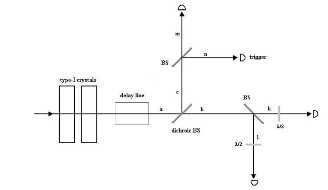
Figure 35: Scheme for the generation and the detection of the four-photon entangled state $|\Phi^{(4)}\rangle$.

If the photon $l_{sq}$ is measured in the computational basis $\{|H\rangle,|V\rangle\}$ with the result $|V\rangle$, then the entangled state is projected onto the state

$$\frac{1}{2}\left[\kappa_{1}^{2}k_{sV}^{{\dagger}}m_{iH}^{{\dagger}}n_{iH}^{{\dagger}}+\frac{1}{2}\kappa_{1}\kappa_{2}k_{sH}^{{\dagger}}(m_{iH}^{{\dagger}}n_{iV}^{{\dagger}}+m_{iV}^{{\dagger}}n_{iH}^{{\dagger}})\right]|0\rangle\;,$$ (455)

which, after normalization, and by setting $\kappa_{2}=2\kappa_{1}$, reduces to a three-photon $W$ state. All the multiphoton multipartite entangled states discussed above have been proposed for various applications in quantum information. In particular, the GHZ- and $W$-class states have been proposed for quantum teleportation with high nonclassical fidelity [614], dense coding [615], quantum secret sharing [616], and quantum key distribution [617].
Multipartite entanglement has been experimentally demonstrated also for continuous variables [618, 619]. In fact, tripartite entangled states have been generated by combining three independent squeezed vacuum states [618], or by manipulating an EPR state with linear optical devices [619]. In the context of nonlinear optics, a multistep interaction model has been proposed as source of three-photon entangled states of the form [620]

$$|\Psi_{3ph}\rangle\,=\,\sum_{k_{1},k_{2},k_{3}}F(k_{1},k_{2},k_{3})a_{1}^{{\dagger}}(k_{1})a_{2}^{{\dagger}}(k_{2})a_{3}^{{\dagger}}(k_{3})|000\rangle\;,$$ (456)

where $F$ is the three-photon spectral function. The state (456) can be generated through two independent down conversion processes and a subsequent up conversion process (sum-frequency generation) inside the same crystal illuminated by a classical pump. In the down conversion processes two pairs of photons are created; the up conversion process, responsible for the generation of a third photon, is originated by the annihilation of a couple of photons each created by a different down conversion process. The three-photon entangled state $|\Psi_{3ph}\rangle$ can be derived from third order perturbation under conditions of energy conservation and phase matching [620]. Another possible experimental scheme for the generation of a three-photon entangled state using multiphoton processes in nonlinear optical media is based on the four-wave mixing Hamiltonian (132), in which one treats the pump mode as a classical pump, describing a particular form of nondegenerate three-photon down conversion process. In Ref. [621] the experimental feasibility and the phase matching conditions for this process are discussed, and some quantitative estimates are presented in the particular case of a calcite crystal.
Several other proposals based on the exploitation of cascaded nonlinearities have been put forward for the realization of multimode entangled states [286, 622, 623, 624]. Hamiltonians of the form Eq. (192) have been considered for the generation of continuous-variable entangled states. In particular, the realization of multiphoton processes described by Hamiltonian (192), involving a $\beta-BaB_{2}O_{4}$ nonlinear crystal, has been suggested and is supported by some preliminary experimental results [286, 622]. With respect to previous realizations [284], in the above mentioned schemes noncollinear phase matching conditions are satisfied through suitable choices of frequencies and propagation angles. The Hamiltonian (192) admits the following constant of the motion:

$$\Delta=N_{1}(t)-N_{2}(t)-N_{i}(t)\;,$$ (457)

where $N_{j}(t)=\langle a_{j}^{{\dagger}}(t)a_{j}\rangle$. For the initial three-mode vacuum state $|0,0,0\rangle$, one has $\Delta=0$ and $N_{1}(t)=N_{2}(t)+N_{i}(t)$ at all times $t$. By exploiting the conservation law, the evolved state $|\psi^{2step}(t)\rangle$ can be expressed in the form [286]

$$|\psi^{2step}(t)\rangle=e^{-itH_{I}^{2step}}|0,0,0\rangle=\frac{1}{\sqrt{1+N_{1}}}$$

$$\times\sum_{m,n}\left(\frac{N_{2}}{1+N_{1}}\right)^{m/2}\left(\frac{N_{i}}{1+N_{1}}\right)^{n/2}\left[\frac{(m+n)!}{m!n!}\right]^{1/2}|n+m,m,n\rangle\;.$$ (458)

The three-mode entangled state (458) can be used to achieve optimal telecloning of coherent states [286]. Another cascaded scheme has been investigated in Ref. [623], based on the following symmetrized three-mode interaction Hamiltonian

$$H_{3CV}\,=\,ir(a_{1}^{{\dagger}}a_{2}^{{\dagger}}+a_{2}^{{\dagger}}a_{3}^{{\dagger}}+a_{3}^{{\dagger}}a_{1}^{{\dagger}})+H.c.\;.$$ (459)

The Heisenberg equations yield the following relations for the quadrature operators

$$X_{1}(t)-X_{2}(t)=(X_{1}-X_{2})e^{-rt}\,,$$

$$X_{1}(t)-X_{3}(t)=(X_{1}-X_{3})e^{-rt}\,,$$

$$P_{1}(t)+P_{2}(t)+P_{3}(t)=(P_{1}+P_{2}+P_{3})e^{-2rt}\,,$$ (460)

whose common eigenstate, in the limit of infinite squeezing $rt\rightarrow\infty$, is the continuous variable GHZ state

$$|\Psi_{GHZ_{3}}\rangle\,=\,\frac{1}{(2\pi)^{3/2}}\int|x\rangle_{1}|x\rangle_{2}|x\rangle_{3}\;.$$ (461)

The infinite squeezing limit is of course unrealistic. However, at finite squeezing, the continuous variable infinitely entangled three-mode GHZ state can be very well approximated by pure symmetric three-mode Gaussian states with sufficiently high, but finite, degree of squeezing [625]. These states enjoy several nice properties, as, in particular, the fact of possessing at the same time maximal genuine tripartite entanglement and maximal bipartite entanglement in all possible two-mode reduced states if one of the original three modes is lost. For this reason, at variance with their three-qubit counterparts, these continuous variable states allow a promiscuous entanglement sharing, and have been therefore named continuous-variable GHZ/$W$ states [625].
The procedure illustrated above for the production of entangled states of three modes can be easily extended to entangle an arbitrary number of modes [623]. In this general case the entangling Hamiltonian becomes

$$H_{NCV}\,=\,ir\sum_{i=1}^{N}\sum_{j>1}^{N}a_{i}^{{\dagger}}a_{j}^{{\dagger}}\,+\,H.c.\;,$$ (462)

and the joint operators are given by

$$\sum_{i=1}^{N}P_{i}(t)\,=\,e^{-(N+1)rt}\sum_{i=1}^{N}P_{i}\;,$$

$$X_{i}(t)-X_{j}(t)\,=\,e^{-rt}(X_{i}-X_{j})\;,\qquad i\neq j\;.$$ (463)

The time evolution generated by this Hamiltonian is able to realize for asymptotically large times or asymptotically large squeezing the continuous variable $N$-mode entangled GHZ state. The effective feasibility of the scheme based on Hamiltonian $H_{NCV}$ has been investigated for $N=3,4$, by resorting to quasi-phase matching techniques, and the simultaneous concurrence of different nonlinearities has been experimentally observed in periodically poled $RbTiOAsO_{4}$ [623].

7.4 Quantum repeaters and quantum memory of light

The main scope of quantum communication is the transmission of quantum states between distant sites, a task that is particularly suited for systems of continuous variables. For instance, it can be in principle easily accomplished by resorting to photonic channels, the main source of troubles in a realistic application being that the error probability scales with the length $l$ of the channel. For instance, in an optical fiber the probability for absorption and depolarization of a photon grows exponentially with the length of the fiber. The fidelity $\mathcal{F}$ of the transmitted state decays exponentially with $l$, i.e. $\mathcal{F}\propto e^{-\gamma l}$, with $\gamma$ being the characteristic decoherence rate; in the same way, decoherence deteriorates entanglement [626]. Hence, long-distance communication appears to be unrealistic, or at least extremely difficult to achieve. The standard purification schemes [510, 627, 628] are not sufficient to circumvent this problem, because they require a threshold value of the fidelity $\mathcal{F}_{min}$ to operate, and the latter is not achievable for increasing $l$.
However, an interesting strategy to solve this probleme has been recently proposed [629], based on the idea of quantum repeaters [630]. The strategy works as follows. Given a long channel, connecting two end sites $A$ and $B$, one can divide it into $N$ segments, with $N$ such that the length $l/N$ of each segment allows to support, between the nodes $A$ and $C_{1}$, $C_{1}$ and $C_{2}$, $\ldots$, $C_{N-1}$ and $B$, EPR pairs with sufficiently high initial fidelity, satisfying $\mathcal{F}_{min}<\mathcal{F}\leq\mathcal{F}_{max}$. Here, $\mathcal{F}_{max}$ denotes the maximum attainable fidelity, and the end points of the intermediate segments $C_{i}$ $(i=1,\ldots,N-1)$ are named auxiliary nodes. After successful purification, all the EPR pairs between $A$ and $B$ are connected by performing Bell measurements at each node $C_{i}$, and the result of this measurement is classically communicated to the next node. At the end, a shared maximally entangled state between $A$ and $B$ has been obtained. This process is called entanglement swapping [631]. A quantum repeater is thus based on a nested purification protocol, combining entanglement swapping and purification [630]. It can be shown that the resources necessary for the efficient functioning of the protocol grow only polynomially with $N$. This is a crucial property for the succesfull implementation of the scheme.
In Ref. [632], an interesting proposal has been put forward for the realization of a quantum repeater by combining linear optical operations and a “double-photon gun”. The “double-photon gun” is defined as a source of a single polarization-entangled photon pair at a time, on demand, and with very high output fidelity. This is a theoretical concept, however proposals for possible experimental realizations do exist. For instance, an example of this source of entanglement has been propesed by Benson et al. [633]. It is based on a semiconductor quantum dot in which the electron-hole recombination leads to the production of a single entangled photon pair, with the advantage of vanishing probability of creating multiple pairs.
In general, the implementation of a quantum repeater, and of other quantum information devices, such as linear optical elements for quantum computation, requires suitable quantum memories. A quantum memory is a device that realizes the task of storing an unknown quantum state of light with a fidelity higher than that of the classical recording. Considering coherent states as the states to be stored, the classical memorization cannot overcome 50 per cent fidelity. Examples of classical memories of light have been experimentally realized exploiting the electromagnetically induced transparency [634, 635]. Quantum memories should allow a memorization of coherent states of light with nonclassical fidelity, i.e. above the 50 per cent classical limit. Several designes of quantum memories have been proposed in Refs. [636, 637, 638, 639]. Experimentally, important progress has been achieved in Refs. [640, 641], while the definitive experimental demonstration of quantum memory of light has been realized by storing coherent states of light onto quantum states of atomic ensembles with 70 per cent fidelity [642].
In the experiments of Refs. [640, 641], the quantum correlations of photon pairs were generated in the collective emission from an atomic ensemble with a controlled time delay. These experiments have accomplished the task of controlled entanglement between atoms and light, but are not yet examples of quantum memory devices obeying the following two fundamental requirements: 1) the state of light sent by a third party must be unknown to the memory (atomic) party; 2) the state of light is transferred in a quantum state (atomic state) of the memory device with nonclassical fidelity. From this point of view, the results reported Ref. [642] are of particular relevance. In this experiment, satisfying the two above criteria, a coherent state of light is stored in the superposition of magnetic sublevels of the ground state of an ensemble of cesium atoms. The experimental setup is schematically depicted in Fig. (36).

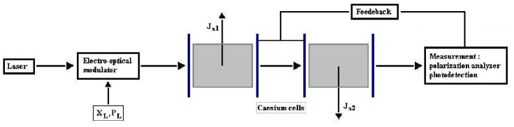
Figure 36: Experimental setup for the realization of a quantum memory of light. The electro-optic modulator is used to generate an input field with arbitrary displacements $X_{L}$ and $P_{L}$. The input field is encoded in the $y$ component of a $x-y$ polarization-entangled state. The two samples of cesium vapor are placed in paraffin-coated glass cells; the cells, placed inside magnetic shields, constitute the storage units. The bias magnetic field $\mathbf{H}$ along the $x$ axis allows for encoding the memory at the Larmor frequency $\Omega$. The canonical quadratures are detected by a polarization state analyzer and by lock-in detection of the $\Omega$-component of the photocurrent.

The objective of the experiment is the storage of the values of the two quadrature operators $X_{L}$ and $P_{L}$ characterizing an, in principle, arbitrary input quantum state (a coherent state in the concrete experimental realization). The $y$-polarized input quantum field $a(t)$ is generated by an electro-optic modulator, and, before crossing an array of paraffin-coated cells, is mixed, on a polarizing beam splitter, with a strong entangling $x$-polarized pulse with photon flux $n(t)$. The two samples of cesium atomic vapors are placed in a bias magnetic field $\mathbf{H}$ oriented along the $x$ axis; moreover, the atomic ensemble is prepared in states that are approximatively coherent spin states, with the $x$ projection $J_{x1}=-J_{x2}=J_{x}=F\,N_{at}$, where $F$ is the collective magnetic moment, and $N_{at}$ is the number of atoms. The array of the two cells allows to introduce the canonical variables for the two ensembles $X_{A}=(J_{y1}-J_{y2})/\sqrt{2J_{x}}$, and $P_{A}=(J_{z1}+J_{z2})/\sqrt{2J_{x}}$. The light is transmitted through the atomic samples. By considering the evolution of the Stokes operators, it can be shown that in the presence of $\mathbf{H}$, the memory couples to the $\Omega$-sidebands of light: $X_{L}=T^{-1/2}\int_{0}^{T}dt\,(a^{{\dagger}}(t)+a(t))\cos(\Omega t)$ and $P_{L}=iT^{-1/2}\int_{0}^{T}dt\,(a^{{\dagger}}(t)-a(t))\cos(\Omega t)$, with $a(t)$ normalized to the photon flux, and $T$ being the pulse duration. $X_{L}$ and $P_{L}$ are detected by a polarization state analyzer and by lock-in detection of the $\Omega$-component of the photocurrent. The polarization measurement of the transmitted light is followed by the feedback onto atoms by means of a radio-frequency magnetic pulse conditioned on the measurement result. At the end, the desired mapping of the input quadratures onto the atom-memory canonical variables, i.e. $X_{L}^{in}\rightarrow-P_{A}^{mem}$, $P_{L}^{in}\rightarrow X_{A}^{mem}$, is realized; thus, the quantum storage is achieved [642]. Let us note that this result has been obtained utilizing coherent states of light as input states; however, since any arbitrary quantum state can be written in terms of a superposition of coherent states, the approach has in principle a completely general validity. Further proposals for the improvement of the above protocol have been put forward in Refs. [643, 644].

8 Conclusions and outlook

Quantum optics plays a key role in several branches of modern physics, involving conceptual foundations and applicative fallouts as well, ranging from fundamental quantum mechanics to lasers and astronomical observation. To understand the vast and complex structure of quantum optics, it is sufficient to list the phenomena that heavily involve multiphoton processes: among them, ionization processes, spontaneous emission, photo-association/dissociation of molecules, quantum interference, quantum tunneling, quantum diffusion, quantum dissipation, shaping of potentials, heating of plasmas, and parametric processes in nonlinear media.
In this review, we have chosen to concentrate our attention on those multiphoton processes that can be exploited to engineer nonclassical and/or entangled states of light. We are motivated by the fact that nonclassical states of light can be considered a fundamental resource in a wide range of applications, from quantum interferometry to more recent and very promising fields of research such as quantum information and quantum communication. Besides the Fock states, the prototypes of nonclassical states of light are the celebrated two-photon squeezed states, that can be generated, for instance, by two-photon down-conversion processes. Therefore, we have mainly considered the multiphoton parametric processes occurring in nonlinear media, that can constitute a useful device for producing new multiphoton quantum states with appealing nonclassical properties that can include and extend the ones exhibited by the two-photon squeezed states.
In the first part of this review we have discussed as well the difficulties in implementing processes associated to susceptibilities of higher nonlinear order, and the possible remarkable enhancements of these quantities that could be achieved by exploiting the recent successes in the engineering of new composite and layered materials. Besides the parametric processes, we have discussed other methods for the generation of multiphoton quantum states, based on the combination either of linear optics or of cavity fields with quantum nondemolition (QND) measurements. Furthermore, we have tried to give a sufficiently broad and fairly complete review of the existing theoretical methods proposed for the definition of different types and classes of multiphoton nonclassical states, and we have briefly discussed the production of multiphoton entangled states and their applications in the rapidly growing research area of quantum computation and information.
The reader should be aware of the fact that, due to limitations in length and scopes, we have often discussed effective Hamiltonian models and realization schemes for multiphoton states under the assumption of devices with ideal efficiency and/or in the absence of losses and dissipation. However, during the time evolution of a real quantum system, the unavoidable interaction with the environment will in general induce loss of phase coherence between the constituent states of the system itself: this phenomenon is known as phase damping, or decoherence [645, 646]. In quantum optics, the influence of amplitude damping, dissipation, and quantum noise on the statistical properties of a quantum open system can be investigated by using different approaches. A first family includes phenomenological master equations for the density matrix and classical Fokker-Planck equations for the corresponding quasi-probability distributions, or Langevin equations. including stochastic forces [20, 22, 172, 647]. Microscopic approaches are also widely used, based on tracing out environmental degrees of freedom in suitable system $+$ bath models [648], and, finally, many of these different descriptions find often an harmonic merging in the axiomatic theory based on the mathematical structure of completely positive dynamical maps and semigroups, and the Lindblad-Skraus superoperators [408, 649, 650, 651]. It is important to keep in mind a clear distinction between decoherence and amplitude damping, especially because the former may often take place on much shorter time scales than the latter, and moreover can be realized by interactions with minimal environments. Methods and schemes to produce multiphoton nonclassical and entangled states via nonlinear interactions in media and cavities are then threatened by the disruptive effects of decoherence and dissipation. In recent years many strategies have been devised to protect quantum systems from losses and dissipation. These strategies, based on quantum control implemented by active feedback mechanisms [652], or by passive protections like decoherence-free subspaces [653], open realistic perspectives, in reasonable times, at least for partial solutions of the problems related to dissipation and decoherence.
In conclusion, we would like to comment on some possible future directions in the physics of multiphoton processes and in the applications of multiphoton states. A first direction will surely concern the theoretical modelling and the experimental realization of larger, better, and more stable (against noise and decoherence) quantum superposition states of the radiation field. Multiphoton coherent and squeezed states of high nonlinear order would be required for such a task, and therefore the attempts to obtain strongly enhanced nonlinear susceptibilities of higher order should play an increasingly important role in this field of research. Another important directions will be along the route to the understanding of the nature of quantum correlations between many parties, and a better understanding of the entanglement properties of multimode multiphoton nonclassical states together with their experimental realizations would be very important tools in the study of multipartite entanglement and, more generally, of fundamental quantum theory. Finally, besides these important conceptual and foundational aspects, realization of larger and better multiphoton nonclassical states should allow further, and partly unexplored, chances and perspectives to quantum optical realizations of quantum information and communication processes.

Aknowledgments

We acknowledge financial support from MIUR under project ex 60%, INFN, and Coherentia CNR-INFM.

References

- [1] P. A. M. Dirac, Proc. Roy. Soc. (London), Ser. A, 114, 243 (1927).
- [2] P. A. M. Dirac, Proc. Roy. Soc. A 117, 610 (1928); P. A. M. Dirac, Proc. Roy. Soc. A 118, 351 (1928).
- [3] W. Heisenberg and W. Pauli, Z. Phys. 56, (1929).
- [4] E. Fermi, Rev. Mod. Phys. 4, 87 (1932).
- [5] R. P. Feynman Phys. Rev. 76, 769 (1949); R. P. Feynman, Phys. Rev. 80, 440 (1950).
- [6] J. S. Schwinger, Phys. Rev. 73, 416 (1948); J. S. Schwinger, Phys. Rev. 74, 1439 (1948); J. S. Schwinger, Phys. Rev. 75, 651 (1949); J. S. Schwinger, Phys. Rev. 76, 790 (1949).
- [7] S. I. Tomonaga, Progr. Theoret. Phys. (Kyoto) 1, 27 (1946).
- [8] S. S. Schweber, An Introduction to Relativistic Quantum Field Theory (Dover, New York, 2005).
- [9] J. D. Bjorken and S. D. Drell, Relativistic Quantum Fields (McGraw-Hill, New York, 1965).
- [10] C. Itzykson and J.-B. Zuber, Quantum Field Theory (Dover, New York, 2005).
- [11] S. Weinberg, The Quantum Theory of Fields (Cambridge University Press, Cambridge, 1995).
- [12] T. H. Maiman, Nature 187, 493 (1960).
- [13] R. J. Glauber, Phys. Rev. Lett. 10, 84 (1963).
- [14] R. J. Glauber, Phys. Rev. 130, 2529 (1963).
- [15] R. J. Glauber, Phys. Rev. 131, 2766 (1963).
- [16] E. C. G. Sudarshan, Phys. Rev. Lett. 10, 277 (1963).
- [17] J. R. Klauder, Ann. Phys. 11, 123 (1960).
- [18] J. R. Klauder and E. C. G. Sudarshan, Fundamentals of quantum optics (Benjamin, New York, 1968).
- [19] J. R. Klauder and B-S Skagerstam, Coherent states (World Scientific, Copenhagen, 1984).
- [20] W. H. Louisell, Quantum Statistical Properties of Radiation (Wiley, New York, 1973).
- [21] L. Mandel and E. Wolf, Optical Coherence and Quantum Optics (Cambridge University Press, Cambridge, 1995).
- [22] D. F. Walls and G. J. Milburn, Quantum Optics (Springer, Berlin, 1994).
- [23] S. M. Barnett and P. M. Radmore, Methods in Theoretical Quantum Optics (Clarendon press, Oxford, 1997).
- [24] M. O. Scully and M. S. Zubairy, Quantum Optics (Cambridge University Press, Cambridge, 1997).
- [25] R. Loudon, The Quantum Theory of Light (Oxford University Press, Oxford, 2000).
- [26] P. Meystre and M. Sargent, Elements of Quantum Optics (Springer, Berlin, 1998).
- [27] R. R. Puri, Mathematical Methods of Quantum Optics (Springer, Berlin, 2001).
- [28] H. A. Haus, Electromagnetic Noise and Quantum Optical Measurements (Springer, Berlin, 2000).
- [29] P. W. Milonni, The Quantum Vacuum: An Introduction to quantum electrodynamics (Academic Press, London, S. Diego, 1994).
- [30] A. Yariv, Quantum Electronics (Wiley, New York, 1989)
- [31] R. Hanbury Brown and R. Twiss, Nature 177 27 (1956).
- [32] G. A. Rebka and R. V. Pound, Nature 180, 1035 (1957).
- [33] E. M. Purcell, Nature 178, 1449 (1956).
- [34] L. Mandel and E. Wolf, Phys. Rev. 124, 1696 (1961).
- [35] E. Schrödinger, Naturwissenschaften 14, 664 (1926).
- [36] U. M. Titulaer and R. J. Glauber, Phys. Rev. 145, 1041 (1966).
- [37] H. Paul, Rev. Mod. Phys. 54, 1061 (1982).
- [38] R. Loudon, Rep. Prog. Phys. 43, 913 (1980).
- [39] X. T. Zou and L. Mandel, Phys. Rev. A 41, 475 (1990).
- [40] L. Davidovich, Rev. Mod. Phys. 68, 127 (1996).
- [41] L. Mandel, Opt. Lett. 4, 205 (1979).
- [42] K. E. Cahill and R. J. Glauber, Phys. Rev. 177, 1857 (1969); K. E. Cahill and R. J. Glauber, Phys. Rev. 177, 1882 (1969).
- [43] K. Husimi, Proc. Phys. Math. Soc. Jpn. 23, 264 (1949).
- [44] E. P. Wigner, Phys. Rev. 40, 749 (1932).
- [45] M. Hillery, R. F. O’Connell, M. O. Scully, and E. P. Wigner, Phys. Rep. 106, 123 (1984).
- [46] A. Kenfack and K. Życzkowski, J. Opt. B: Quantum Semiclass. Opt. 6, 396 (2004).
- [47] K. Vogel and H. Risken, Phys. Rev. A 40, 2847 (1989).
- [48] H. P. Yuen and V. W. S. Chan, Opt. Lett. 8, 177 (1983).
- [49] G. L. Abbas, V. W. S. Chan, and S. T. Yee, Opt. Lett. 8, 419 (1983).
- [50] G. M. D’Ariano, C. Macchiavello, and M. G. A. Paris, Phys. Rev. A 50, 4298 (1994).
- [51] G. M. D’Ariano, U. Leonhardt, and H. Paul, Phys. Rev. A 52, R1801 (1995).
- [52] U. Leonhardt, Measuring the Quantum State of Light (Cambridge University Press, Cambridge, 1997).
- [53] D. T. Smithey, M. Beck, M. G. Raymer, and A. Faridani, Phys. Rev. Lett. 70, 1244 (1993).
- [54] G. Breitenbach, S. Schiller, and J. Mlynek, Nature 387, 471 (1997).
- [55] C. Kurtsiefer, T. Pfau, and J. Mlynek, Nature 386, 150 (1997).
- [56] G. Breitenbach, F. Illuminati, S. Schiller, and J. Mlynek, Europhys. Lett. 44, 192 (1998).
- [57] J. H. Shapiro and S. S. Wagner, IEEE J. Quantum Electron. QE-20, 803 (1984).
- [58] H. P. Yuen and J. H. Shapiro, IEEE Trans. Inf. Theory IT-26, 78 (1980).
- [59] P. A. Franken, A. E. Hill, C. W. Peters, and G. Weinreich, Phys. Rev. Lett. 7, 118 (1961).
- [60] G. S. He and S. H. Liu, Physics of nonlinear optics (World Scientific, 1999).
- [61] N. Bloembergen, Nonlinear optics (Benjamin, 1965).
- [62] Y. R. Shen, The Principles of Nonlinear Optics (Wiley-Interscience, 1984).
- [63] P. N. Butcher and D. Cotter, The elements of nonlinear optics (Cambridge University Press, 1990).
- [64] R. W. Boyd, Nonlinear Optics (Academic Press).
- [65] W. E. Lamb, Jr., Phys. Rev. 85, 259 (1952).
- [66] H. Haken, Z. Phys. 181, 96 (1964).
- [67] K. H. Yang, Ann. Phys. (NY) 101, 62 (1976).
- [68] D. H. Kobe, Phys. Rev. Lett. 40, 538 (1978); D. H. Kobe and A. L. Smirl, Am. J. Phys. 46, 624 (1978).
- [69] G. Grynberg and E. Giacobino, J. Phys. B 12, L93 (1979).
- [70] L. Mandel, Phys. Rev. A 20, 1590 (1979).
- [71] W. Becker, Opt. Commun. 56, 107 (1985).
- [72] P. D. Drummond, Phys. Rev. A 35, 4253 (1987).
- [73] M. Born and L. Infeld, Pro. R. Soc. London, Ser. A 147, 522 (1934); ibidem 150, 141 (1935).
- [74] J. M. Jauch and K. M. Watson, Phys. Rev. 74, 950 (1948).
- [75] Y. R. Shen, Phys. Rev. 155, 921 (1967).
- [76] J Tucker and D. F. Walls, Phys. Rev. 178, 2036 (1969).
- [77] G. Nienhuis and C. Th. J. Alkemade, Physica C 81, 181 (1976).
- [78] M. Hillery and L. D. Mlodinow, Phys. Rev. A 30, 1860 (1984).
- [79] I. Abram, Phys. Rev. A 35, 4661 (1987).
- [80] L. Knöll, W. Vogel, and D. G. Welsch, Phys. Rev. A 36, 3803 (1988).
- [81] P. D. Drummond, Phys. Rev. A 42, 6845 (1990).
- [82] R. J. Glauber and M. Lewenstein, Phys. Rev. A 43, 467 (1991).
- [83] I. Abram and E. Cohen, Phys. Rev. A 44, 500 (1991).
- [84] B. Huttner, J. J. Baumberg, and S. M. Barnett, Europhys. Lett. 16, 177 (1991); B. Huttner and S. M. Barnett, Europhys. Lett. 18, 487 (1992).
- [85] D. J. Santos and R. Loudon, Phys. Rev. A 52, 1538 (1995).
- [86] T. Gruner and D. G. Welsch, Phys. Rev. A 51, 3246 (1995).
- [87] R. Matloob, R. Loudon, S. M. Barnett, and J. Jeffers, Phys. Rev. A 52, 4823 (1995); R. Matloob and R. Loudon, Phys. Rev. A 53, 4567 (1996).
- [88] L. Duan and G. Guo, Phys. Rev. A 56, 925 (1997).
- [89] T. K. Yee and T. K. Gustafson, Phys. Rev. A 18, 1597 (1978).
- [90] D. A. Kleinman, Phys. Rev. 126, 1977 (1962).
- [91] R. W. Boyd, J. Mod. Opt. 46, 367 (1999).
- [92] G. L. Fischer, R. W. Boyd, R. J. Gehr, S. A. Jenekhe, J. A. Osaheni, J. E. Sipe, and L. A. Weller-Brophy, Phys. Rev. Lett. 74, 1871 (1995).
- [93] N. N. Lepeshkin, A. Schweinsberg, G. Piredda, R. S. Bennik, and R. W. Boyd, Phys. Rev. Lett. 93, 123902 (2004).
- [94] R. del Coso, J. Requejo-Isidro, J. Solis, J. Gonzalo, and C. N. Afonso, J. Appl. Phys. 95, 2755 (2004).
- [95] H. B. Liao, R. F. Xiao, H. Wang, K. S. Wong, and G. K. L. Wong, Appl. Phys. Lett. 72, 1817 (1998).
- [96] A. N. Naumov, A. B. Fedotov, A. M. Zheltikov, V. V. Yakovlev, L. A. Mel’nikov, V. I. Beloglazov, N. B. Skibina, and A. V. Shcherbakov, J. Opt. Soc. Am. B 19, 2183 (2002).
- [97] P. P. Markowicz, H. Tiryaki, H. Pudavar, and P. N. Prasad, Phys. Rev. Lett. 92, 083903 (2004).
- [98] R. De Salvo, D. J. Hagan, M. Sheik-Bahae, G. Stegeman, E. W. Van Stryland, and H. Vanherzeele, Opt. Lett. 17, 28 (1992).
- [99] G. I. Stegeman, M. Sheik-Bahae, E. Van Stryland, and G. Assanto, Opt. Lett. 18, 13 (1993).
- [100] G. I. Stegeman, D. J. Hagan, and L. Torner, Opt. Quantum Electron. 28, 1691 (1996).
- [101] X. D. Mu, X. Gu, M. V. Makarov, Y. J. Ding, J. Wang, J. Wei, Y. Liu, Opt. Lett. 25, 117 (2000).
- [102] H. Crespo, J. T. Mendonca, and A. Dos Santos, Opt. Lett. 25, 829 (2000).
- [103] L. Misoguti, S. Backus, C. G. Durfee, R. Bartels, M. M. Murnane, and H. C. Kapteyn, Phys. Rev. Lett. 87, 013601 (2001).
- [104] G. Alzetta, A. Gozzini, L. Moi, G. Orriols, Nuovo Cimento B36, 5 (1976).
- [105] E. Arimondo, Progress in Optics, Vol. XXXV (Elsevier Science, Amsterdam, 1996).
- [106] A. Imamoğlu and S. E. Harris, Opt. Lett. 14, 1344 (1989).
- [107] S. E. Harris, Phys. Today 50, 36 (1997).
- [108] S. E. Harris, J. E. Field, and A. Imamoğlu, Phys. Rev. Lett. 64, 1107 (1990).
- [109] M. D. Lukin and A. Imamoğlu, Nature 413, 273 (2001).
- [110] , K.-J. Boller, A. Imamoğlu, and S. E. Harris, Phys. Rev. Lett. 66, 2593 (1991).
- [111] S. E. Harris and L. V. Hau, Phys. Rev. Lett. 82, 4611 (1999).
- [112] M. D. Lukin and A. Imamoğlu, Phys. Rev. Lett. 84, 1419 (2000).
- [113] A. B. Matsko, I. Novikova, G. R. Welch, and M. S. Zubairy, Opt. Lett. 28, 96 (2003).
- [114] K. Hakuta, L. Marmet, and B. P. Stoicheff, Phys. Rev. Lett. 66, 596 (1991).
- [115] G. Z. Zhang, K. Hakuta, and B. P. Stoicheff, Phys. Rev. Lett. 71, 3099 (1993).
- [116] H. Kang and Y. Zhu, Phys. Rev. Lett. 91, 093601 (2003).
- [117] M. S. Zubairy, A. B. Matsko, and M. O. Scully, Phys. Rev. A 65, 043804 (2002).
- [118] J. A. Giordmaine, Phys. Rev. Lett. 8, 19 (1962).
- [119] P. D. Maker, R. W. Terhune, M. Nisenoff, and C. M. Savage, Phys. Rev. Lett. 8, 21 (1962).
- [120] J. E. Midwinter and J. Warner, Brit. J. Appl. Phys. 16, 1135 (1965).
- [121] J. E. Midwinter and J. Warner, Brit. J. Appl. Phys. 16, 1667 (1965).
- [122] M. V. Hobden, J. Appl. Phys. 38, 4365 (1967).
- [123] H. Ito, H. Naito, and H. Inaba, J. Appl. Phys. 46, 3992 (1975).
- [124] H. Rabin and P. P. Bey, Phys. Rev. 156, 1010 (1967); P. P. Bey and H. Rabin, Phys. Rev. 162, 794 (1967).
- [125] J. T. Murray, N. Peyghambarian, R. C. Powell, R. A. Stolzenberger, S. Jie, and B. Jassemnejad, Phys. Rev. A 49, 4066 (1994).
- [126] J. A. Armstrong, N. Bloembergen, J. Ducuing, and P. S. Pershan, Phys. Rev. 127, 1918 (1962).
- [127] P. A. Franken and J. F. Ward, Rev. Mod. Phys. 35, 23 (1963).
- [128] V. Pruneri, S. D. Butterwoth, and D. C. Hanna, Opt. Lett. 21, 390 (1996); C. J. van der Poel, J. D. Bierlien, J. B. Brown, and S. Colak, Appl. Phys. Lett. 57 2074 (1990); G. Khanarian, R. A. Norwood, D. Haas, B. Feuer, and D. Karim, Appl. Phys. Lett. 57, 977 (1990); M. S. Pitch, C. D. Cantrell, and R. C. Sce, J. Appl. Phys. 47, 3514 (1976); A. Szilagyi, A. Hordvik, and H. Schlossberg, J. Appl. Phys. 47, 2055 (1976).
- [129] S. Zhu, Y. Zhu, Y. Qin, H. Wang, C. Ge, and N. Ming, Phys. Rev. Lett. 78, 2752 (1997).
- [130] S. Zhu, Y. Zhu, N. Ming, Science 278, 843 (1997).
- [131] W. H. Louisell, A. Yariv, and A. E. Siegman, Phys. Rev. 124, 1646 (1961).
- [132] J. P. Gordon, W. H. Louisell, and L. R. Walker, Phys. Rev. 129, 481 (1963).
- [133] B. R. Mollow and R. J. Glauber, Phys. Rev. 160, 1077 (1967); B. R. Mollow and R. J. Glauber, Phys. Rev. 160, 1097 (1967).
- [134] J. Tucker and D. F. Walls, Ann. Phys. (N.Y.) 52, 1 (1969).
- [135] D. C. Burnham and D. L. Weinberg, Phys. Rev. Lett. 25, 84 (1970).
- [136] S. Friberg and L. Mandel, J. Opt. Soc. Am. 74, 101 (1984); S. Friberg, C. K. Hong, and L. Mandel, Phys. Rev. Lett. 54, 2011 (1985).
- [137] H. P. Yuen and J. H. Shapiro, Opt. Lett. 4, 334 (1979).
- [138] B. Yurke, Phys. Rev. A 32, 300 (1985).
- [139] R. S. Bondurant, P. Kumar, J. H. Shapiro, and M. Maeda, Phys. Rev. A 30, 343 (1984).
- [140] M. D. Levenson, R. M. Shelby, A. Aspect, M. D. Reid, and D. F. Walls, Phys. Rev. A 32, 1550 (1985); M. D. Levenson, R. M. Shelby, and S. H. Perlmutter, Opt. Lett. 10, 514 (1985); R. M. Shelby, M. D. Levenson, D. F. Walls, G. J. Milburn, and A. Aspect, Phys. Rev. A 33, 4008 (1986).
- [141] R. E. Slusher, L. W. Hollberg, B. Yurke, J. C. Mertz, and J. F. Valley, Phys. Rev. A 31, 3512 (1985); R. E. Slusher, L. W. Hollberg, B. Yurke, J. C. Mertz, and J. F. Valley, Phys. Rev. Lett. 55, 2409 (1985).
- [142] M. Hillery and M. S. Zubairy, Phys. Rev. A 29, 1275 (1984).
- [143] G. Scharf and D. F. Walls, Opt. Commun. 50, 245 (1984).
- [144] D. D. Crouch and S. L. Braunstein, Phys. Rev. A 38, 4696 (1988).
- [145] M. G. A. Paris, Phys. Lett. A 217, 78 (1996).
- [146] G. M. D’Ariano, M. G. A. Paris, and M. F. Sacchi, Il Nuovo Cimento 114, 339 (1999).
- [147] D. F. Walls and R. Barakat, Phys. Rev. A 1, 446 (1970).
- [148] G. P. Agrawal and C. L. Mehta, J. Phys. A: Math., Nucl. Gen. 7, 607 (1974).
- [149] R. Gambini, Phys. Rev. A 15, 1157 (1977).
- [150] S. Kumar and C. L. Mehta, Phys. Rev. A 21, 1573 (1980).
- [151] J. Katriel and D. G. Hummer, J. Phys. A: Math. Gen. 14, 1211 (1981).
- [152] K. J. McNiel and C. W. Gardiner, Phys. Rev. A 28, 1560 (1983).
- [153] B. Jurčo, J. Math. Phys. 30, 1739 (1989).
- [154] S. Carusotto, Phys. Rev. A 40, 1848 (1989).
- [155] G. Drobný and I. Jex, Phys. Rev. A 46, 499 (1992); I. Jex and G. Drobný, J. Mod. Opt. 39, 1043 (1992).
- [156] G. Drobný, I. Jex, and V. Bužek, Phys. Rev. A 48, 569 (1993).
- [157] P. Kinsler, M. Fernée, and P. D. Drummond, Phys. Rev. A 48, 3310 (1993).
- [158] M. Hillery, D. Yu, and J. Bergou, Phys. Rev. A 52, 3209 (1995).
- [159] M. Fernée, P. Kinsler, and P. D. Drummond, Phys. Rev. A 51, 864 (1995).
- [160] A. Bandilla, G. Drobný and I. Jex, Phys. Rev. Lett. 75, 4019 (1995); A. Bandilla, G. Drobný and I. Jex, Phys. Rev. A 53, 507 (1996); A. Bandilla, G. Drobný and I. Jex, Opt. Commun. 128, 353 (1996).
- [161] C. Brif, Phys. Rev. A 54, 5253 (1996).
- [162] J. M. Manley and H. E. Rowe, Proc. IRE 44, 904 (1956).
- [163] R. A. Brandt and O. W. Greenberg, J. Math. Phys. 10, 1168 (1969).
- [164] M. Rasetti, Int. J. Theor. Phys. 5, 377 (1972).
- [165] V. Bargmann, Ann. Math. 48, 568 (1947).
- [166] J. Katriel, Phys. Lett. A 34, 44 (1971).
- [167] D. F. Walls and C. T. Tindle, J. Phys. A 5, 534 (1972).
- [168] J. Mostowski and K. Rza̧żewski, Phys. Lett. A 66, 275 (1978).
- [169] M. Hillery, D. Yu, and J. Bergou, Phys. Rev. A 49, 1288 (1994).
- [170] N. Cohen and S. L. Braunstein, Phys. Rev. A 52, 815 (1995).
- [171] M. D. Reid and D. F. Walls, Phys. Rev. A 34, 4929 (1986).
- [172] J. Perina, Quantum statistics of linear and nonlinear optical phenomena (Kluwer Academic Publishers, 1991).
- [173] J-L. Oudar and Y. R. Shen, Phys. Rev. A 22, 1141 (1980).
- [174] N. Bloembergen, Nobel lecture, (1981).
- [175] D. K. Giri and P. S. Gupta, J. Opt. B: Quantum Semiclass. Opt. 6, 91 (2004).
- [176] L. Deng, M. Kozuma, E. W. Hagley, and M. G. Payne, Phys. Rev. Lett. 88, 143902 (2002).
- [177] M. T. Johnsson and M. Fleischhauer, Phys. Rev. A 66, 043808 (2002).
- [178] M. T. Johnsson and M. Fleischhauer, Phys. Rev. A 68, 023804 (2003).
- [179] Y. Wu, J. Saldana, and Y. Zhu, Phys. Rev. A 67, 013811 (2003).
- [180] Y. Wu and X. Yang, Phys. Rev. A 70, 053818 (2004).
- [181] D. A. Braje, V. Balić, S. Goda, G. Y. Yin, and S. E. Harris, Phys. Rev. Lett. 93, 183601 (2004).
- [182] H. Kang, G. Hernandez, and Y. Zhu, Phys. Rev. A 70, 061804 (2004).
- [183] V. A. Andreev and Q. A. Ivanova, J. Phys. A 35, 8587 (2001).
- [184] Y. Wu and X. Yang, Opt. Lett. 29, 839 (2004).
- [185] Y. Wu, X. Yang, and Y. Xiao, Phys. Rev. Lett. 86, 2200 (2001).
- [186] H. P. Yuen, Phys. Rev. A 13, 2226 (1976).
- [187] D. F. Walls, Nature 306, 141 (1983).
- [188] C. M. Caves and B. L. Schumaker, Phys. Rev. A 31, 3068 (1985); B. L. Schumaker and C. M. Caves, Phys. Rev. A 31, 3093 (1985).
- [189] Y. Yamamoto and H. A. Haus, Rev. Mod. Phys. 58, 1001 (1986).
- [190] R. Bonifacio and G. Preparata, Phys. Rev. A 2, 336 (1970).
- [191] T. von Forester and R. J. Glauber, Phys. Rev. A 3, 1484 (1971).
- [192] E. Y. C. Lu, Phys. Rev. A 8, 1053 (1973).
- [193] G. P. Agrawal and C. L. Metha, Phys. Rev. A 12, 1513 (1975).
- [194] F. Persico and G. Vetri, Phys. Rev. A 12, 2083 (1975).
- [195] D. F. Walls, and P. Zoller, Phys. Rev. Lett. 47, 709 (1981); R. Loudon, Opt. Commun. 49, 24 (1984).
- [196] W. Becker, M. O. Scully, and M. S. Zubairy, Phys. Rev. Lett. 48, 475 (1982); C. Sibilia, M. Bertolotti, V. Perǐnová, J. Peřina, and A. Lukš, Phys. Rev. A 28, 328 (1983).
- [197] L. Mandel, Opt. Commun. 42, 437 (1982); M. Kozierowski, and S. Kielich, Phys. Lett. A 94, 213 (1983).
- [198] L. A. Lugiato and G. Strini, Opt. Commun. 41, 67 (1982);
- [199] M. S. Zubairy, M. S. K. Razmi, S. Iqbal, and M. Idress, Phys, Lett. A 98, 168 (1983); R. Loudon, Opt. Commun. 49, 67 (1984).
- [200] G. Milburn and D. F. Walls, Opt. Commun. 39, 401 (1981).
- [201] R. E. Slusher, L. W. Hollberg, B. Yurke, J. C. Mertz, and J. F. Valley, Phys. Rev. Lett. 55, 2409 (1985).
- [202] R. M. Shelby, M. D. Levenson, S. H. Perlmutter, R. G. DeVoe, and D. F. Walls, Phys. Rev. Lett. 57, 691 (1986).
- [203] L. A. Wu, H. J. Kimble, J. L. Hall, and H. Wu, Phys. Rev. Lett. 57, 2520 (1986).
- [204] P. Kurz, R. Paschotta, K. Fiedler, A. Sizmann, G. Leuchs, and J. Mlynek, Appl. Phys. B 55, 216 (1992).
- [205] C. Kim and P. Kumar, Phys. Rev. Lett. 73, 1605 (1994).
- [206] M. Rosenbluh and R. M. Shelby, Phys. Rev. Lett. 66, 153 (1991).
- [207] K. Bergman, C. R. Doerr, H. A. Has, and M. Shirasaki, Opt. Lett. 18, 643 (1993).
- [208] K. Bergman, H. A. Haus, E. P. Ippen, and M. Shirasaki, Opt. Lett. 19, 290 (1994).
- [209] E. S. Polzik, J. Carri, and H. J. Kimble, Appl. Phys. B 55279 (1992).
- [210] A. Heidmann, R. J. Horowicz, S. Reynaud, E. Giacobino, C. Fabre, and G. Camy, Phys. Rev. Lett. 59, 2555 (1987).
- [211] O. Aytür and P. Kumar, Phys. Rev. Lett. 65, 1551 (1990).
- [212] Y.-q. Li and M. Xiao, Opt. Expr. 2, 110 (1998).
- [213] A. Levenson, P. Vidakovic, and C. Simonneau, Pure Appl. Opt. 7, 281 (1998).
- [214] D. Stoler, Phys. Rev. D 1, 3217 (1970).
- [215] C. K. Hong and L. Mandel, Phys. Rev. Lett. 54, 323 (1985).
- [216] W. Schleich and J. A. Wheeler, Nature 326, 574 (1987).
- [217] C. M. Caves, C. Zhu, G. J. Milburn, and W. Schleich, Phys. Rev. A 43, 3854 (1991); G. Schrade, V. M. Akulin, V. I. Man’ko, and W. P. Schleich, Phys. Rev. A 48, 2398 (1993).
- [218] D. T. Pegg and S. M. Barnett, Europhys. Lett. 6, 483 (1988); D. T. Pegg and S. M. Barnett, Phys. Rev. A 39, 1665 (1989).
- [219] S. M. Barnett and D. T. Pegg, J. Mod. Optics 36, 7 (1989).
- [220] D. Stoler, Phys. Rev. Lett. 33, 1397 (1974).
- [221] R. A. Fisher, M. M. Nieto, and V. D. Sandberg, Phys. Rev. D 29, 1107 (1984).
- [222] S. L. Braunstein and R. I. McLachlan, Phys. Rev. A 35, 1659 (1987).
- [223] S. L. Braunstein and C. M. Caves, Phys. Rev. A 42, 4115 (1990).
- [224] P. V. Elyutin and D. N. Klyshko, Phys. Lett. A 149, 241 (1990).
- [225] G. Drobný and I. Jex, Phys. Rev. A 45, 1816 (1992).
- [226] G. Drobný and I. Jex, Phys. Rev. A 45, 4897 (1992).
- [227] R. Tanaś and Ts. Gantsog, Phys. Rev. A 45, 5031 (1992).
- [228] K. Banaszek and P. L. Knight, Phys. Rev. A 55, 2368 (1997).
- [229] T. Felbinger, S. Schiller, and J. Mlynek, Phys. Rev. Lett. 80, 492 (1998).
- [230] V. B. Braginsky and F. Y. Khalili, Rev. Mod. Phys. 68, 1 (1996).
- [231] N. Imoto, H. A. Haus, and Y. Yamamoto, Phys. Rev. A 32, 2287 (1985).
- [232] Y. Yamamoto and A. Imamoḡlu, Mesoscopic Quantum Optics (John Wiley and Sons, Inc, 1999).
- [233] H. H. Ritze and A. Bandilla, Opt. Commun. 29, 126 (1979).
- [234] M. Kitagawa and Y. Yamamoto, Phys. Rev. A 34, 3974 (1986).
- [235] Y. Yamamoto and H. A. Haus, Rev. Mod. Phys. 58, 1001 (1986).
- [236] M. Kitagawa, N. Imoto, and Y. Yamamoto, Phys. Rev. A 35, 5270 (1987).
- [237] N. Imoto and S. Saito, Phys. Rev. A 39, 675 (1989).
- [238] P. Alsing, G. J. Milburn, and D. F. Walls, Phys. Rev. A 37, 2970 (1988).
- [239] A. N. Chaba, M. J. Collett, and D. F. Walls, Phys. Rev. A 46, 1499 (1992).
- [240] M. Genovese and C. Novero, Phys. Rev. A 61, 032102 (2000).
- [241] M. D. Levenson, R. M. Shelby, M. Reid, and D. F. Walls, Phys. Rev. Lett. 57, 2473 (1986).
- [242] S. R. Friberg, S. Machida, and Y. Yamamoto, Phys. Rev. Lett. 69, 3165 (1992).
- [243] P. Grangier, J. F. Roch, and G. Royer, Phys. Rev. Lett. 66, 1418 (1991).
- [244] J. F. Roch, K. Vigneron, Ph. Grelu, A. Sinatra, J. Ph. Poizat, and P. Grangier, Phys. Rev. Lett. 78, 634 (1997).
- [245] S. M. Jensen, IEEE J. Quantum Electron. QE-18, 1580 (1982).
- [246] A. M. Maier, Kvant. Elektron. (Moscow) 9, 2996 (1982).
- [247] A. Chefles and S. M. Barnett, J. Mod. Opt. 43, 709 (1996).
- [248] N. Korolkova and J. Peřina, Opt. Commun. 136, 135 (1997).
- [249] A-B. M. A. Ibrahim, B. A. Umarov, and M. R. B. Wahiddin, Phys. Rev. A 61, 043804 (2000).
- [250] G. Ariunbold and J. Peřina, Opt. Commun. 176, 149 (2000).
- [251] W. Leoński and A. Miranowicz, J. Opt. B: Quantum Semiclass. Opt. 6, S37 (2004).
- [252] W. Leoński, Phys. Rev. A 55, 3874 (1997).
- [253] A. Miranowicz and W. Leoński, J. Opt. B: Quantum Semiclass. Opt. 6, S43 (2004).
- [254] D. T. Pegg, L. S. Phillips, and S. M. Barnett, Phys. Rev. Lett. 81, 1604 (1998); S. M. Barnett and D. T. Pegg, Phys. Rev. A 60, 4965 (1999).
- [255] B. C. Sanders, Phys. Rev. A 45, 6811 (1992).
- [256] B. C. Sanders and D. A. Rice, Phys. Rev. A 61, 013805 (1999).
- [257] C. C. Gerry and R. A. Campos, Phys. Rev. A 64, 063814 (2001).
- [258] C. C. Gerry and A. Benmoussa, Phys. Rev. A 65, 033822 (2002).
- [259] C. C. Gerry, A. Benmoussa, and R. A. Campos, Phys. Rev. A 66, 013804 (2002).
- [260] E. Fredkin and T. Toffoli, Int. J. Theor. Phys. 21, 905 (1982); G. J. Milburn, Phys. Rev. Lett. 62, 2124 (1989).
- [261] J. J. Bollinger, W. M. Itano, D. J. Wineland, and D. J. Heinzen, Phys. Rev. A 54, R4649 (1996).
- [262] M. J. Holland and K. Burnett, Phys. Rev. Lett. 71, 1355 (1993).
- [263] M. W. Mitchell, J. S. Lundeen, and A. M. Steinberg, Nature 429, 161 (2004).
- [264] P. Walther, J.-W. Pan, M. Aspelmeyer, R. Ursin, S. Gasparoni, and A. Zeilinger, Nature 429, 158 (2004).
- [265] S. Song, C. M. Caves, and B. Yurke, Phys. Rev. A 41, 5261 (1990); B. Sherman and G. Kurizki, Phys. Rev. A 45, R7674 (1992).
- [266] L. Davidovich, M. Brune, J. M. Raimond, and S. Haroche, Phys. Rev. A 53, 1295 (1996); M. Brune, E. Hagley, J. Dreyel, X. Maitre, A. Maali, C. Wunderlich, J. M. Raimond, and S. Haroche, Phys. Rev. Lett. 77, 4887 (1996); P. Tombesi and D. Vitali, Phys. Rev. Lett. 77, 411 (1996).
- [267] G. J. Milburn, Phys. Rev. A 33, 674 (1986); G. J. Milburn and C. A. Holmes, Phys. Rev. Lett. 56, 2237 (1986).
- [268] B. Yurke and D. Stoler, Phys. Rev. Lett. 57, 13 (1986).
- [269] A. Mecozzi and P. Tombesi, Phys. Rev. Lett. 58, 1055 (1987).
- [270] B. Yurke and D. Stoler, Phys. Rev. A 35, 4846 (1987).
- [271] G. C. Gerry, Opt. Commun. 63, 278 (1987); Ts. Gantsog and R. Tanaś, Quantum Opt. 3, 33 (1991).
- [272] W. Schleich, M. Pernigo, and Fam Le Kien, Phys. Rev. A 44, 2172 (1991).
- [273] G. S. Agarwal and K. Tara, Phys. Rev. A 46, 485 (1992).
- [274] K. Tara, G. S. Agarwal, and S. Chaturvedi, Phys. Rev. A 47, 5024 (1993).
- [275] R. Tanaś, in Coherence and Quantum Optics V, edited by L. Mandel and E. Wolf (Plenum, New York, 1984).
- [276] S. Du, S. Gong, Z. Xu, L. Zhou, and C. Gong, Opt. Commun. 138, 193 (1997).
- [277] G. S. Agarwal and R. R. Puri, Phys. Rev. A 40, 5179 (1989).
- [278] D. Mogilevtsev and K. S. Ya, Opt. Commun. 132, 452 (1996).
- [279] H. Jeong, M. S. Kim, T. C. Ralph, and B. S. Ham, Phys. Rev. A 70, 061801(R) (2004).
- [280] P. Tombesi and H. P. Yuen, in Coherence and Quantum Optics V, edited by L. Mandel and E. Wolf (Plenum, New York, 1984).
- [281] C. C. Gerry and S. Rodrigues, Phys. Rev. A 36, 5444 (1987).
- [282] G. Y. Kryuchkyan and K. V. Kheruntsyan, Opt. Commun. 127, 230 (1996).
- [283] C. Cabrillo and F. J. Bermejo, Phys. Rev. A 48, 2433 (1993); K. V. Kheruntsyan, D. S. Krähmer, G. Y. Kryuchkyan, and K. G. Petrossian, Opt. Commun. 139, 157 (1997).
- [284] R. A. Andrews, H. Rabin, and C. L. Tang, Phys. Rev. Lett. 25, 605 (1970).
- [285] M. E. Smithers and E. Y. C. Lu, Phys. Rev. A 10, 1874 (1974).
- [286] A. Ferraro, M. G. A. Paris, M. Bondani, A. Allevi, E. Puddu, and A. Andreoni, J. Opt. Soc. Am. B 21, 1241 (2004).
- [287] M. A. M. Marte, Phys. Rev. Lett. 74, 4815 (1995).
- [288] A. G. White, P. K. Lam, M. S. Taubman, M. A. M. Marte, S. Schiller, D. E. McClelland, and H.-A. Bachor, Phys. Rev. A 55, 4511 (1997).
- [289] A. L. Aleksandrovski, A. S. Chirkin, and V. V. Volkov, J. Russ. Laser Res. 18, 101 (1997); A. S. Chirkin, V. V. Volkov, G. D. Laptev, and E. Y. Morozov, Quantum Electron. 30, 847 (2000); A. V. Nikandrov and A. S. Chirkin, JETP Lett. 76, 275 (2002).
- [290] A. S. Chirkin, J. Opt. B: Quantum Semiclass. Opt. 4, S91 (2002); A. S. Chirkin and A. V. Nikandrov, J. Opt. B: Quantum Semiclass. Opt. 5, 169 (2003).
- [291] A. V. Nikandrov and A. S. Chirkin, J. Russ. Laser Res. 23, 81 (2002).
- [292] Z. Y. Ou, L. J. Wang, X. Y. Zou, and L. Mandel, Phys. Rev. A 41, 566 (1990).
- [293] X. Y. Zou, L. J. Wang, and L. Mandel, Phys. Rev. Lett. 67, 318 (1991); X. Y. Zou, T. Grayson, G. A. Barbosa, and L. Mandel, Phys. Rev. A 47, 2293 (1993).
- [294] A. V. Burlakov, M. V. Chekhova, D. N. Klyshko, S. P. Kulik, A. N. Penin, Y. H. Shih, and D. V. Strekalov, Phys. Rev. A 56, 3214 (1997).
- [295] P. G. Kwiat, E. Waks, A. G. White, I. Appelbaum, and P. H. Eberhard, Phys. Rev. A, 60, R773 (1999).
- [296] M. Atatüre, A. V. Sergienko, B. E. A. Saleh, and M. C. Teich, Phys. Rev. Lett. 86, 4013 (2001).
- [297] G. Di Giuseppe, M. Atatüre, M. D. Shaw, A. V. Sergienko, B. E. A. Saleh, and M. C. Teich, Phys. Rev. A 66, 013801 (2002).
- [298] A. Luis and J. Peřina, Phys. Rev. A 53, 1886 (1996).
- [299] G. M. D’Ariano, M. G. A. Paris, and M. F. Sacchi, Phys. Rev. A 57, 4894 (1998).
- [300] J. H. Shapiro, S. R. Shepard, and N. W. Wong, Phys. Rev. Lett. 62, 2377 (1991); J. H. Shapiro and S. R. Shepard, Phys. Rev. A 43, 3795 (1991).
- [301] F. De Martini, Phys. Rev. Lett. 81, 2842 (1998); F. De Martini, Phys. Lett. A 250, 15 (1998).
- [302] F. De Martini, M. Fortunato, P. Tombesi, and D. Vitali, Phys. Rev. A 60, 1636 (1999).
- [303] H. Fan and G. Yu, Phys. Rev. A 65, 033829 (2002).
- [304] G. Yu. Kryuchkyan and N. T. Muradyan, Phys. Lett. A 286, 113 (2001).
- [305] K. Molmer, Y. Castin, J. Dalibard, J. Opt. Soc. Am. B 10, 524 (1993).
- [306] M. B. Plenio and P. L. Knight, Rev. Mod. Phys. 70, 101 (1998).
- [307] K. V. Kheruntsyan, G. Yu. Kryuchkyan, N. T. Mouradyan, and K. G. Petrosyan, Phys. Rev. A 57, 535 (1998).
- [308] V. V. Dodonov, J. Opt. B: Quantum Semiclass. Opt. 4, R1 (2002).
- [309] V. V. Dodonov, Theory of Non-classical States of Light (Taylor & Francis, London, New York, 2003)
- [310] M. D. Reid and D. F. Walls, Phys. Rev. Lett. 53, 955 (1984); M. D. Reid and D. F. Walls, Phys. Rev. A 34, 1260 (1986).
- [311] J. R. Klauder, J. Math. Phys. 4, 1055 (1963); J. R. Klauder, J. Math. Phys. 4, 1058 (1963).
- [312] A. M. Perelomov, Commun. Math. Phys. 26, 222 (1972); A. M. Perelomov, Generalized Coherent States and Their Applications (Springer, Berlin, 1986).
- [313] R. Gilmore, Ann. Phys. 74, 391 (1972); R. Gilmore, Lie Groups, Lie Algebras and Some of Their Applications (Wiley, New York, 1974).
- [314] A. O. Barut and L. Girardello, Commun. Math. Phys. 21, 41 (1971).
- [315] V. V. Dodonov, I. A. Malkin, and V. I. Man’ko, Physica 72, 597 (1974); H. Hillery, Phys. Rev. A 36, 3796 (1987).
- [316] G. S. Agarwal, Phys. Rev. Lett. 57, 827 (1986); G. S. Agarwal, J. Opt. Soc. Am. B 5, 1940 (1988).
- [317] N. B. An and T. M. Duc, J. Opt. B: Quantum Semiclass. Opt. 4, 80 (2002); N. B. An, J. Opt. B: Quantum Semiclass. Opt. 4, 222 (2002).
- [318] V. I. Man’ko, G. Marmo, S. Solimeno, and F. Zaccaria, Int. J. Mod. Phys. A 8, 3577 (1993).
- [319] G. S. Prakash and G. S. Agarwal, Phys. Rev. A 50, 4258 (1994); G. S. Prakash and G. S. Agarwal, Phys. Rev. A 52, 2335 (1995).
- [320] C. Brif, Ann. Phys. NY 251, 180 (1996).
- [321] C. Aragone, G. Guerri, S. Salamo, and J. L. Tani, J. Phys. A: Math. Gen. 7, L149 (1974); C. Aragone, E. Chalbaud, and S. Salamo, J. Math. Phys. 17, 1963 (1976).
- [322] M. M. Nieto and D. R. Truax, Phys. Rev. Lett. 71, 2843 (1993).
- [323] R. R. Puri, Phys. Rev. A 49, 2178 (1994).
- [324] C. C. Gerry and R. Grobe, Phys. Rev. A 51, 4123 (1995).
- [325] W. Zhang, D. Feng, and R. Gilmore, Rev. Mod. Phys. 62 867 (1990).
- [326] V. P. Karassiov, J. Sov. Laser Res. 13, 188, (1992).
- [327] V. Sunilkumar, B. A. Bambah, R. Jagannathan, P. K. Panigrahi, and V. Srinivasan, J. Opt. B 2, 126 (2000).
- [328] N. Debergh, J. Phys. A: Math. Gen. 31, 4013 (1998).
- [329] R. L. de Matos Filho and W. Vogel, Phys. Rev. A 54 4560 (1996).
- [330] V. I. Man’ko, G. Marmo, E. C. G. Sudarshan, and F. Zaccaria, Phys. Scr. 55, 528 (1997).
- [331] E. Roy and P. Roy, J. Opt. B: Quantum Semiclass. Opt. 2, 65 (2000).
- [332] L. C. Kwek and D. Kiang, J. Opt. B: Quantum Semiclass. Opt. 5, 383 (2000).
- [333] P. Shanta, S. Chaturvedi, V. Srinivasan, and G. S. Agarwal, Phys. Rev. Lett. 72, 1447 (1994).
- [334] G. D’Ariano, M. Rasetti, and M. Vadacchino, Phys. Rev. D 32, 1034 (1985); G. D’Ariano and M. Rasetti, Phys. Rev. D 35, 1239 (1987).
- [335] J. Katriel, A. Solomon, G. D’Ariano, and M. Rasetti, Phys. Rev. D 34, 2332 (1986); J. Katriel, M. Rasetti, and A. I. Solomon, Phys. Rev. D 35, 1248 (1987); J. Katriel, M. Rasetti, and A. I. Solomon, Phys. Rev. D 35, 2601 (1987).
- [336] P. Tombesi and A. Mecozzi, Phys. Rev. A 37, 4778 (1988).
- [337] M. Hillery, Phys. Rev. A 42, 498 (1990).
- [338] V. Bužek and G. Drobný, Phys. Rev. A 47, 1237 (1993).
- [339] G. Drobný and V. Bužek, Phys. Rev. A 50, 3492 (1994).
- [340] R. Graham, Phys. Rev. Lett. 52, 117 (1984).
- [341] T. Holstein and H. Primakoff, Phys. Rev. 58, 1048 (1940).
- [342] G. A. Baker, Jr. and P. Graves-Morris, Padé approximants, Enciclopedia of Mathematics and its Applications (No. 59), 2nd Edition (Cambridge University Press, Cambridge, 1996).
- [343] M. Araki and E. Lieb, Commun. Math. 18, 160 (1970).
- [344] Y. Wu and X. Yang, Opt. Lett. 28, 1793 (2003).
- [345] Y. Wu and X. Yang, J. Opt. B: Quantum Semiclass. Opt. 6, 184 (2004).
- [346] B. T. H. Varcoe, S. Brattke, M. Weidinger, and H. Walther, Nature 403, 743 (2000); S. Brattke, B. T. H. Varcoe, and H. Walther, Phys. Rev. Lett. 86, 3534 (2001).
- [347] J. Krause, M. O. Scully, and H. Walther, Phys. Rev. A 36, 4547 (1987); J. Krause, M. O. Scully, T. Walther, and H. Walther, Phys. Rev. A 39, 1915 (1989).
- [348] M. Brune, S. Haroche, V. Lefevre, J. M. Raimond, and N. Zagury, Phys. Rev. Lett. 65, 976 (1990).
- [349] J. M. Kublinski, Phys. Rev. Lett. 64, 2507 (1990).
- [350] M. J. Holland, D. F. Walls, and P. Zoller, Phys. Rev. Lett. 67, 1716 (1991).
- [351] K. Vogel, V. M. Akulin, and W. P. Schleich, Phys. Rev. Lett. 71, 1816 (1993).
- [352] S. Y. Kilin and D. B. Horosko, Phys. Rev. Lett. 74, 5206 (1995).
- [353] W. Leoński, Phys. Rev. A 54, 3369 (1995).
- [354] G. M. D’Ariano, L. Maccone, M. G. A. Paris, and M. F. Sacchi, Phys. Rev. A 61, 053817 (2000).
- [355] K. Sanaka, Phys. Rev. A 71, 021801(R) (2005).
- [356] M. V. Satyanarayana, Phys. Rev. D 32, 400 (1985).
- [357] M. S. Kim, F. A. M. de Oliveira, and P. L. Knight, Opt. Commun. 72, 99 (1989); M. S. Kim, F. A. M. de Oliveira, and P. L. Knight, Phys. Rev. A 40, 2494 (1989); F. A. M. de Oliveira, M. S. Kim, P. L. Knight, and V. Bužek, Phys. Rev. A 41, 2645 (1990).
- [358] P. Král, J. Mod. Opt. 37, 889 (1990).
- [359] P. Marian, Phys. Rev. A 44, 3325 (1991).
- [360] K. B. Møller, T. G. Jørgensen, and J. P. Dahl, Phys. Rev. A 54, 5378 (1996).
- [361] M. M. Nieto, Phys. Lett. A 229, 135 (1997).
- [362] C. F. Lo, Phys. Rev. A 43, 404 (1991).
- [363] I. Földesi, P. Adam, J. Janszky, Phys. Lett. A 204, 16 (1995).
- [364] L. Albano, D. F. Mundarain, and J. Stephany, J. Opt. B: Quantum Semiclass. Opt. 4, 352 (2002).
- [365] G. M. Abd Al-Kader, J. Opt. B: Quantum Semiclass. Opt. 5, S228 (2003).
- [366] P. Král, Phys. Rev. A 42, 4177 (1990).
- [367] A. I. Lvovsky and S. A. Babichev, Phys. Rev. A 66, 011801 (2002).
- [368] A. D. Wilson-Gordon, V. Bužek, and P. L. Knight, Phys. Rev. A 44, 7647 (1991).
- [369] K. Sundar, Phys. Rev. A 53, 1096 (1996).
- [370] C. C. Gerry and R. Grobe, Phys. Rev. A 49, 2033 (1994).
- [371] V. Peřinová, V. Vrana, A. Lukš, and J. Křepelka, Phys. Rev. A 51, 2499 (1995).
- [372] D. Stoler, B. E. A. Saleh, and M. C. Teich, Opt. Acta 32, 345 (1985).
- [373] C. T. Lee, Phys. Rev. A 31, 1213 (1985).
- [374] A. Vidiella-Barranco and J. A. Roversi, Phys. Rev. A 50, 5233 (1994).
- [375] G. Dattoli, J. Gallardo, and A. Torre, J. Opt. Soc. Am. B 2, 185 (1987).
- [376] H.Y. Fan and N.L. Liu, Phys. Lett. A 264, 154 (1999).
- [377] A. Joshi and S. V. Lawande, Opt. Commun. 70, 21 (1989); A. Joshi and S. V. Lawande, J. Mod. Opt. 38, 2009 (1991).
- [378] K. Matsuo, Phys. Rev. A 41, 519 (1990).
- [379] R. D’Souza and A. P. Mishra, Phys. Rev. A 45, 6925 (1992).
- [380] G. S. Agarwal, Phys. Rev. A 45, 1787 (1992).
- [381] S. M. Barnett, J. Mod. Opt. 45, 2201 (1998).
- [382] X. G. Wang, S. H. Pan, and G. Z. Yang, Euro. Phys. J. D 10, 415 (2000).
- [383] G. C. Guo and S. B. Zheng, Phys. Lett. A 223, 332 (1996).
- [384] J. Liao, X. Wang, L.A. Wu, and S.H. Pan, J. Opt. B: Quantum Semiclass. Opt. 3, 302 (2001).
- [385] S. M. Barnett and D. T. Pegg, Phys. Rev. Lett. 76, 4148 (1996).
- [386] M. H. Y. Moussa and B. Baseia, Phys. Lett. A 238, 223 (1998).
- [387] R. Simon and M. V. Satyanarayana, J. Mod. Opt. 35, 719 (1988).
- [388] H. C. Fu and R. Sasaki, J. Math. Phys. 38,3968 (1997).
- [389] G. S. Agarwal and K. Tara, Phys. Rev. A 43, 492 (1991).
- [390] G. Bjork and Y. Yamamoto, Phys. Rev. A 37, 4229 (1988).
- [391] V. V. Dodonov, M. A. Marchiolli, Y. A. Korennoy, V. I. Man’ko, and Y. A. Moukhin, Phys. Rev. A 58, 4087 (1998).
- [392] Z. Zhang and H. Fan, Phys. Lett. A 165, 14 (1992).
- [393] V. V. Dodonov, Y. A. Korennoy, V. I. Man’ko, and Y. A. Moukhin, Quantum Semiclassic. Opt. 8, 413 (1996).
- [394] G. S. Agarwal and K. Tara, Phys. Rev. A 46, 485 (1992); G. N. Jones, J. Haight, and C. T. Lee, Quantum Semiclassic. Opt. 9, 411 (1997).
- [395] M. Dakna, T. Anhut, T. Opatrný, L. Knöll, and D. G. Welsch, Phys. Rev. A 55, 3184 (1997).
- [396] M. S. Kim, E. Park, P. L. Knight, and H. Jeong, Phys. Rev. A 71, 043805 (2005).
- [397] M. Ban, J. Mod. Opt. 43, 1281 (1996).
- [398] L. Hong, Phys. Lett. A 264, 265 (1999).
- [399] G. S. Agarwal, R. R. Puri, and R. P. Singh, Phys. Rev. A 56, 4207 (1997).
- [400] V. Bužek, I. Jex, and T. Quang, J. Mod. Opt. 37, 159 (1990); I. Jex and V. Bužek, J. Mod. Opt. 40, 771 (1993).
- [401] J. Sun, J Wang, and C. Wang, Phys. Rev. A 44, 3369 (1991); J. Sun, J. Wang, and C. Wang, Phys. Rev. A 46, 1700 (1992).
- [402] M. M. Nieto and D. R. Truax, Phys. Lett. A 208, 8 (1995); M. M. Nieto and D. R. Truax, Opt. Commun. 179, 197 (2000).
- [403] Z. M. Zhang, L. Xu, J. L. Chai, and F. L. Li, Phys. Lett. A 150, 27 (1990).
- [404] I. Jex, P. Törmä, and S. Stenholm, J. Mod. Opt. 42, 1377 (1995).
- [405] P. Marian, Phys. Rev. A 55, 3051 (1997).
- [406] Z. Z. Xin, D. B. Wang, M. Hirayama, and K. Matumoto, Phys. Rev. A 50, 2865 (1994); A. S.F. Obada and Z. M. Omar, Phys. Lett. A 227, 349 (1997).
- [407] J. J. Slosser, P. Meystre, and S. L. Braunstein, Phys. Rev. Lett. 63, 934 (1989); J. J. Slosser and P. Meystre, Phys. Rev. A 41, 3867 (1990).
- [408] E. B. Davies, Quantum Theory of Open Systems, (Academy Press, London, 1976).
- [409] J. J. Slosser, P. Meystre, and E. Wright, Opt. Lett. 15, 233 (1990).
- [410] P. Meystre, J. J. Slosser, and M Wilkens, Phys. Rev. A 43, 4959 (1991).
- [411] H. P. Yuen, Phys. Rev. Lett. 56, 2176 (1986).
- [412] P. R. Tapster, J. G. Rarity, and J. S. Satchell, Phys. Rev. A 37, 2963 (1988).
- [413] K. Watanabe and Y. Yamamoto, Phys. Rev. A 38, 3556 (1988).
- [414] M. Ueda, N. Imoto, and T. Ogawa, Phys. Rev. A 41, 6331 (1990).
- [415] M. Ban, Phys. Lett. A 233, 284 (1997).
- [416] A. Luis and L. L. Sánchez-Soto, Phys. Lett. A 244, 211 (1998).
- [417] A. I. Lvovsky, H. Hansen, T. Aichele, O. Benson, J. Mlynek, and S. Schiller, Phys. Rev. Lett. 87, 050402 (2001).
- [418] M. G. A. Paris, Phys. Lett. A 289, 167 (2001).
- [419] J. Fiurás̆ek, Phys. Rev. A 64, 053817 (2001).
- [420] A. Zavatta, S. Viciani, and M. Bellini, Science 306, 660 (2004).
- [421] J. Wenger, R. Tualle-Brouri, and P. Grangier, Phys. Rev. Lett. 92, 153601 (2004).
- [422] K. J. Resch, J. S. Lundeen, and A. M. Steinberg, Phys. Rev. Lett. 88, 113601 (2002).
- [423] F. De Martini, V. Mussi, and F. Bovino, Opt. Commun. 179, 581 (2000).
- [424] A. Lamas-Linares, C. Simon, J. C. Howell, and D. Bouwmeester, Science 296, 712 (2002).
- [425] J. Laurat, T. Coudreau, N. Treps, A. Maître, and C. Fabre, Phys. Rev. Lett. 91, 213601 (2003).
- [426] J. Laurat, T. Coudreau, N. Treps, A. Maître, and C. Fabre, Phys. Rev. A 69, 033808 (2004).
- [427] P. Meystre, J. J. Slosser, and M. Wilkens, Opt. Commun. 79, 300 (1990).
- [428] C. M. Savage, S. L. Braunstein, and D. F. Walls, Opt. Lett. 15, 628 (1990).
- [429] B. Sherman and G. Kurizki, Phys. Rev. A 45, R7674 (1992).
- [430] B. M. Garraway, B. Sherman, H. Moya-Cessa, P. L. Knight, and G. Kurizki, Phys. Rev. A 49, 535 (1994).
- [431] M. Brune, J. M. Raimond, and S. Haroche, Phys. Rev. A 35, 154 (1987).
- [432] A. H. Toor and M. S. Zubairy, Phys. Rev. A 45, 4951 (1992).
- [433] M. Brune, E. Hagley, J. Dreyer, X. Maître, A. Maali, C. Wunderlich, J. M. Raimond, and S. Haroche, Phys. Rev. Lett. 77, 4887 (1996).
- [434] J. M. Raimond, M. Brune, and S. Haroche, Phys. Rev. Lett. 79, 1964 (1997).
- [435] J. M. Raimond, M. Brune, and S. Haroche, Rev. Mod. Phys. 73, 565 (2001).
- [436] C. K. Law and J. H. Eberly, Phys. Rev. Lett. 76, 1055 (1996).
- [437] R. M. Serra, N. G. de Almeida, C. J. Villas-Bôas, and M. H. Y. Moussa, Phys. Rev. A 62, 043810 (2000).
- [438] J. Janszky, P. Domokos, S. Szabo, and P. Adam, Phys. Rev. A 51, 4191 (1995).
- [439] S. Szabo, P. Adam, J. Janszky, and P. Domokos, Phys. Rev. A 53, 2698 (1996).
- [440] M. Dakna, L. Knöll, D.-G. Welsch, Opt. Commun. 145, 309 (1998).
- [441] M. Dakna, L. Knöll, D.-G. Welsch, Eur. Phys. J. D. 3, 295 (1998).
- [442] M. Dakna, J. Clausen, L. Knöll, D.-G. Welsch, Phys. Rev. A 59, 1658 (1999); M. Dakna, J. Clausen, L. Knöll, D.-G. Welsch, Phys. Rev. A 60, 726 (1999).
- [443] C. Valverde, A. T. Avelar, B. Baseia, and J. M. C. Malbouisson, Phys. Lett. A 315, 213 (2003).
- [444] S. Souza, A. T. Avelar, N. G. de Almeida, B. Baseia, Opt. Commun. 239, 359 (2004).
- [445] J. Fiurášek, R. García-Patrón, and N. J. Cerf, Phys. Rev. A 72, 033822 (2005).
- [446] W. Leoński, Phys. Rev. A 55, 3874 (1997).
- [447] V. Bužek, A. D. Wilson-Gordon, P. L. Knight, and W. K. Lai, Phys. Rev. A 45, 8079 (1992).
- [448] A. Miranowicz, K. Pia̧tek, and R. Tanaś, Phys. Rev. A 50, 3423 (1994).
- [449] A. Vidiella-Barranco and J. A. Roversi, Phys. Rev. A 58, 3349 (1998).
- [450] M. G. A. Paris, M. Cola, and R. Bonifacio, Phys. Rev. A 67, 042104 (2003).
- [451] N. G. de Almeida, R. M. Serra, C. J. Villas-Bôas, and M. H. Y. Moussa, Phys. Rev. A 69, 035802 (2004).
- [452] M. Paternostro, M. S. Kim, and B. S. Ham, J. Mod. Opt. 50, 2565 (2003); M. Paternostro, M. S. Kim, and B. S. Ham, Phys. Rev. A 67, 023811 (2003).
- [453] C. K. Hong and L. Mandel, Phys. Rev. A 32, 974 (1985).
- [454] R. Short and L. Mandel, Phys. Rev. Lett. 51, 384 (1983).
- [455] S. Schiller, G. Breitenbach, S. F. Pereira, T. Müller, and J. Mlynek, Phys. Rev. Lett. 77, 2933 (1996).
- [456] M. Hillery, Phys. Rev. A 35, 725 (1987); M. Hillery, Phys. Rev. A 39, 2994 (1989).
- [457] V. V. Dodonov, O. V. Man’ko, V. I. Man’ko, and A. Wünsche, J. Mod. Opt. 47, 633 (2000).
- [458] P. Marian, T. A. Marian, and H. Scutaru, Phys. Rev. Lett. 88, 153601 (2002); P. Marian, T. A. Marian, and H. Scutaru, Phys. Rev. A 68, 062309 (2003).
- [459] K. Życzkowski and W. Slomczyński, J. Phys. A: Math. Gen. 31, 9095 (1998); K. Życzkowski and W. Slomczyński, J. Phys. A: Math. Gen. 34, 6689 (2001).
- [460] I. Bialynicki-Birula, M. A. Cirone, J. P. Dahl, M. Fedorov, and W. P. Schleich, Phys. Rev. Lett. 89, 0604041 (2002).
- [461] C. T. Lee, Phys. Rev. A 44, R2775 (1991); C. T. Lee, Phys. Rev. A 45, 6586 (1992).
- [462] N. Lutkenhaus and St. M. Barnett, Phys. Rev. A 51, 3340 (1995).
- [463] J. Janszky, M. G. Kim, and M. S. Kim, Phys. Rev. A 53, 502 (1996).
- [464] W. Vogel, Phys. Rev. Lett. 84, 1849 (2000).
- [465] A. I. Lvovsky and J. H. Shapiro, Phys. Rev. A 65, 033830 (2002).
- [466] G. S. Agarwal, Opt. Commun. 95, 109 (1993).
- [467] D. N. Klyshko, Phys. Usp. 37, 1097 (1994); D. N. Klyshko, Phys. Lett. A 213, 7 (1996).
- [468] Arvind, N. Mukunda, and R. Simon, Phys. Rev. A 56, 5042 (1997).
- [469] G. M. D’Ariano, M. F. Sacchi, and P. Kumar, Phys. Rev. A 59, 826 (1999).
- [470] E. Shchukin, Th. Ritcher, and W. Vogel, Phys. Rev. A 71, 011802 (2005).
- [471] E. Shchukin and W. Vogel, Phys. Rev. A 72, 043808 (2005).
- [472] Th. Ritcher and W. Vogel, Phys. Rev. Lett. 89, 283601 (2002).
- [473] J. K. Korbicz, J. I. Cirac, J. Wehr, and M. Lewenstein, Phys. Rev. Lett. 94, 153601 (2005).
- [474] D. Bures, Trans. Am. Math. Soc. 135, 199 (1969); A. Uhlmann, Rep. Math. Phys. 9, 273 (1976).
- [475] L. Diósi, Phys. Rev. Lett. 85, 2841 (2000).
- [476] S. Bochner, Math. Ann. 108, 378 (1933).
- [477] B. Reznick, Real Algebraic Geometry and Ordered Structures, edited by C. N. Delzell and J. J. Madden, Contemporary Mathematics 253 (American Mathematical Society, Providence, 2000).
- [478] J. K. Asbóth, J. Calsamiglia, and H. Ritsch, Phys. Rev. Lett. 94, 173602 (2005).
- [479] F. Dell’Anno, S. De Siena, and F. Illuminati, Phys. Rev. A 69, 033812 (2004).
- [480] F. Dell’Anno, S. De Siena, and F. Illuminati, Phys. Rev. A 69, 033813 (2004).
- [481] S. De Siena, A. Di Lisi, and F. Illuminati, Phys. Rev. A 64, 063803 (2001).
- [482] S. De Siena, A. Di Lisi, and F. Illuminati, J. Phys. B 35, L291 (2002).
- [483] F. Dell’Anno, S. De Siena, A. Di Lisi, and F. Illuminati, Int. J. Mod. Phys. B 18, 633 (2004).
- [484] FanHong-yi and J. R. Klauder, Phys. Rev. A 49, 704 (1994).
- [485] FanHong-yi and FanYue, Phys. Rev. A 54, 958 (1996).
- [486] FanHong-yi, Phys. Rev. A 65, 064102 (2002).
- [487] J. Wei and E. Norman, J. Math. Phys. 4A, 575 (1963).
- [488] D. R. Truax, Phys. Rev. D 31, 1988 (1985).
- [489] G. Dattoli, M. Ricchetta, and A. Torre, Phys. Rev. A 37, 2007 (1988).
- [490] A. Einstein, B. Podolsky, and N. Rosen, Phys. Rev. 47, 777 (1935).
- [491] G. M. D’Ariano and M. F. Sacchi, Phys. Rev. A 52, R4309 (1995).
- [492] M. A. Nielsen and I. L. Chuang, Quantum Computation and Quantum Information (Cambridge University Press, Cambridge, 2000).
- [493] G. Benenti, G. Casati, and G. Strini, Principles of Quantum Computation and Information (World Scientific, Singapore, 2004).
- [494] The Physics of Quantum Information: Quantum Cryptography, Quantum Teleportation, Quantum Computation, edited by D. Bouwmeester, A. K. Ekert, and A. Zeilinger (Springer, Berlin, 2000).
- [495] Fundamentals of Quantum Information, edited by D. Heiss (Springer, Berlin, 2002).
- [496] C. H. Bennett, Phys. Today 48, 24 (1995).
- [497] A. K. Ekert and R. Jozsa, Rev. Mod. Phys. 68, 733 (1996).
- [498] T. P. Spiller, Proc. IEEE 84, 1719 (1996).
- [499] A. Steane, Rep. Prog. Phys. 61, 117 (1998).
- [500] C. H. Bennett and D. P. DiVincenzo, Nature 404, 247 (2000).
- [501] S. L. Braunstein, H.-K. Lo, and P. Kok (Editors), Progr. Phys. 48, 767 (2000).
- [502] N. Gisin, G. Ribordy, W. Tiffel, and H. Zbinden, Rev. Mod. Phys. 74, 145 (2002).
- [503] I. Abram and P. Grangier, C. R. Physique 4, 187 (2003).
- [504] See, e.g., J. I. Cirac, in Fundamentals of Quantum Information, edited by D. Heiss (Springer-Verlag, Heidelberg-Berlin, 2002), and references therein.
- [505] C. H. Bennett, D. P. Di Vincenzo, J. A. Smolin, and W. K. Wootters, Phys. Rev. A 54, 3824 (1996).
- [506] V. Vedral, M. B. Plenio, M. A. Rippin, and P. L. Knight, Phys. Rev. Lett. 78, 2275 (1997).
- [507] V. Vedral, M. B. Plenio, K. Jacobs, and P. L. Knight, Phys. Rev. A 56, 4452 (1997).
- [508] V. Vedral and M. B. Plenio, Phys. Rev. A 57, 1619 (1998).
- [509] G. Vidal and R. F. Werner, Phys. Rev. A 65, 032314 (2002).
- [510] C. H. Bennett, G. Brassard, S. Popescu, B. Schumacher, J. Smolin, and W. K. Wootters, Phys. Rev. Lett. 76, 722 (1996).
- [511] L.-M. Duan, G. Giedke, J. I. Cirac, and P. Zoller Phys. Rev. Lett. 84, 4002 (2000).
- [512] J. W. Pan, C. Simon, C. Brukner, and A. Zeilinger, Nature 410, 1067 (2001).
- [513] M. Horodecki, P. Horodecki, and R. Horodecki, Phys. Rev. Lett. 80, 5239 (1998).
- [514] P. Horodecki and M. Lewenstein, Phys. Rev. Lett. 85, 2657 (2000).
- [515] W. K. Wootters, Phys. Rev. Lett. 80, 2245 (1998).
- [516] G. Giedke, M. M. Wolf, O. Krüger, R. F. Werner, and J. I. Cirac, Phys. Rev. Lett. 91, 107901 (2003).
- [517] M. Horodecki, P. Horodecki, and R. Horodecki, Phys. Rev. Lett. 84, 2014 (2000).
- [518] J. Eisert, PhD Thesis (University of Potsdam, Potsdam, 2001).
- [519] K. Zyczkowski, P. Horodecki, A. Sanpera, and M. Lewenstein, Phys. Rev. A 58, 883 (1998).
- [520] M. B. Plenio, unpublished (2001); Phys. Rev. Lett. 95, 090503 (2005).
- [521] J. Lee, M. S. Kim, Y. J. Park, and S. Lee, J. Mod. Opt. 47, 2157 (2000).
- [522] M. Horodecki, P. Horodecki, and R. Horodecki, Phys. Rev. Lett. 84, 4260 (2000).
- [523] A. Peres, Phys. Rev. Lett. 77, 1413 (1996).
- [524] M. Horodecki, P. Horodecki, and R. Horodecki, Phys. Lett. A 223, 1 (1996); P. Horodecki, Phys. Lett. A 232, 333 (1997).
- [525] R. F. Werner, Phys. Rev. A 40, 4277 (1989).
- [526] R. Simon, Phys. Rev. Lett. 84, 2726 (2000).
- [527] J. Williamson, Am. J. Math. 58, 141 (1936); R. Simon, S. Chaturvedi, and V. Srinivasan, J. Math. Phys. 40, 3632 (1999).
- [528] R. Simon, E. C. G. Sudarshan, and N. Mukunda, Phys. Rev. A 36, 3868 (1987); R. Simon, N. Mukunda, and B. Dutta, Phys. Rev. A 49, 1567 (1994); Arvind, B. Dutta, N. Mukunda, and R. Simon, Pramana 45, 471 (1995), and quant-ph/9509002.
- [529] A. Serafini, F. Illuminati, and S. De Siena, J. Phys. B 37, L21 (2004).
- [530] G. Adesso, A. Serafini, and F. Illuminati, Phys. Rev. Lett. 92, 087901 (2004).
- [531] G. Adesso, A. Serafini, and F. Illuminati, Phys. Rev. A 70, 022318 (2004).
- [532] M. M. Wolf, G. Giedke, O. Krüger, R. F. Werner, and J. I. Cirac, Phys. Rev. A 69, 052320 (2004).
- [533] G. Adesso, and F. Illuminati, Phys. Rev. A 72, 032334 (2005).
- [534] G. Adesso, A. Serafini, and F. Illuminati, Phys. Rev. Lett. 93, 220504 (2004).
- [535] A. Serafini, G. Adesso, and F. Illuminati, Phys. Rev. A 71, 032349 (2005).
- [536] W. Dür, J. I. Cirac, and R. Tarrach, Phys. Rev. Lett. 83, 3562 (1999); W. Dür and J. I. Cirac, Phys. Rev. A 61, 042314 (2000).
- [537] M. D. Reid and P. D. Drummond, Phys. Rev. Lett. 60, 2731 (1988); P. D. Drummond and M. D. Reid, Phys. Rev. A 41, 3930 (1990); M. D. Reid, Phys. Rev. A 40, 913 (1989).
- [538] S. M. Tan, Phys. Rev. A 60, 2752 (1999).
- [539] L.-M. Duan, G. Giedke, J. I. Cirac, and P. Zoller, Phys. Rev. Lett. 84, 2722 (2000).
- [540] G. Giedke, B. Kraus, M. Lewenstein, and, J. I. Cirac, Phys. Rev. Lett. 87, 167904 (2001).
- [541] S. Mancini, V. Giovannetti, D. Vitali, and P. Tombesi, Phys. Rev. Lett. 88, 120401 (2002); V. Giovannetti, S. Mancini, D. Vitali, and P. Tombesi, Phys. Rev. A 67, 022320 (2003).
- [542] M. G. Raymer, A. C. Funk, B. C. Sanders, and H. de Guise, Phys. Rev. A 67, 052104 (2003).
- [543] G. Toth, C. Simon, and J. I. Cirac, Phys. Rev. A 68, 062310 (2003).
- [544] O. V. Man’ko, V. I. Man’ko, G. Marmo, A. Shaji, E. C. G. Sudarshan, and F. Zaccaria, Phys. Lett. A 339, 194 (2005); C. Lupo, V. I. Man’ko, G. Marmo, E. C. G. Sudarshan, J. Phys. A: Gen. Phys. 38, 10377 (2005).
- [545] G. S. Agarwal and A. Biswas, quant-ph/0507144.
- [546] M. Hillery and M. S. Zubairy, quant-ph/0507168.
- [547] E. Shchukin and W. Vogel, Phys. Rev. Lett. 95, 230502 (2005).
- [548] A. Serafini, quant-ph/0508231.
- [549] R. F. Werner and M. M. Wolf, Phys. Rev. Lett. 86, 3658 (2001).
- [550] M. S. Kim, W. Son, V. Bužek, and P. L. Knight, Phys. Rev. A 65, 032323 (2002).
- [551] A. Kitagawa, M. Takeoka, M. Sasaki, and A. Chefles, quant-ph/0512069.
- [552] V. V. Dodonov and L. A. de Souza, J. Opt. B: Quantum Semiclass. Opt. 7, 5490 (2005).
- [553] M. M. Wolf, G. Giedke, and J. I. Cirac, quant-ph/0509154.
- [554] P. T. Cochrane, G. J. Milburn, and W. J. Munro, Phys. Rev. A 59, 2631 (1999).
- [555] H. Jeong and M. S. Kim, Phys. Rev. 65, 042305 (2001).
- [556] P. Benioff, J. Stat. Phys. 29, 515 (1982).
- [557] P. Benioff, Phys. Rev. Lett. 48, 1581 (1982).
- [558] R. P. Feynman, Int. J. Theor. Phys. 21, 467 (1982).
- [559] R. P. Feynman, Opt. News 11, 11 (1985).
- [560] R. P. Feynman, Found. Phys. 16, 507 (1986).
- [561] P. W. Shor, in Proceedings of the 35th Annual Symposium on Foundations of Computer Science (IEEE Press, Los Alamitos, CA, 1994).
- [562] D. Deutsch, Proc. R. Soc. A 400, 97 (1985); D. Deutsch, Proc. R. Soc. A 425, 73 (1989).
- [563] I. L. Chuang and Y. Yamamoto, Phys. Rev. A 52, 3489 (1995).
- [564] E. Knill, R. Laflamme, and G. J. Milburn, Nature 409, 46 (2001).
- [565] D. Gottesman, A, Kitaev, and J. Preskill, Phys. Rev. A 64, 012310 (2001).
- [566] L. K. Grover, Phys. Rev. Lett. 79, 325 (1997).
- [567] K. Nemoto and W. J. Munro, Phys. Rev. Lett. 93, 250502 (2004).
- [568] Quantum Information with Continuous Variables, edited by S. L. Braunstein and A. K. Pati (Kluwer, Dordrecht, 2003).
- [569] S. L. Braunstein and P. van Loock, Rev. Mod. Phys. 77, 513 (2005).
- [570] S. Lloyd and S. L. Braunstein, Phys. Rev. Lett. 82, 1784 (1999).
- [571] S. D. Bartlett and B. C. Sanders, Phys. Rev. A 65, 042304 (2002).
- [572] C. H. Bennett, G. Brassard, C. Crépeau, R. Jozsa, A. Peres, and W. K. Wootters, Phys. Rev. Lett. 70, 1895 (1993).
- [573] L. Vaidman, Phys. Rev. A 49, 1473 (1994).
- [574] S. L. Braunstein and H. J. Kimble, Phys. Rev. Lett. 80, 869 (1998).
- [575] D. Bouwmeester, J.-W. Pan, K. Mattle, M. Eibl, H. Weinfurter, and A. Zeilinger, Nature 390, 575 (1997).
- [576] D. Boschi, S. Branca, F. De Martini, L. Hardy, and S. Popescu, Phys. Rev. Lett. 80, 1121 (1998).
- [577] A. Furusawa, J. L. Sørensen, S. L. Braunstein, C. A. Fuchs, H. J. Kimble, and E. S. Polzik, Science 282, 706 (1998).
- [578] N. Takei, H. Yonezawa, T. Aoki, and A. Furusawa, Phys. Rev. Lett. 94, 220502 (2005).
- [579] D. Gottesman and I. L. Chuang, Nature 402, 390 (1999).
- [580] D. Greenberger, M. Horne, A. Shimony, and A. Zeilinger, Am. J. Phys. 58, 1131 (1990).
- [581] P. G. Kwiat, K. Mattle, H. Weinfurter, A. Zeilinger, A. V. Sergienko, and Y. Shih, Phys. Rev. Lett. 75, 4337 (1995).
- [582] M. J. A. de Dood, W. T. M. Irvine, and D. Bouwmeester, Phys. Rev. Lett. 93, 040504 (2004).
- [583] X. Li, P. L. Voss, J. E. Sharping, and P. Kumar, Phys. Rev. Lett. 94, 053601 (2005).
- [584] N. Lütkenhaus, J. Calsamiglia, and K.-A. Suominen, Phys. Rev. A 59, 3295 (1999).
- [585] P. G. Kwiat and H. Weinfurter, Phys. Rev. A 58, R2623 (1998).
- [586] M. O. Scully, B.-G. Englert, and C. J. Bednar, Phys. Rev. Lett. 83, 4433 (1999).
- [587] D. Vitali, M. Fortunato, and P. Tombesi, Phys. Rev. Lett. 85, 445 (2000).
- [588] S. D. Barrett, P. Kok, K. Nemoto, R. G. Beausoleil, W. J. Munro, and T. P. Spiller, Phys. Rev. A 71, 060302(R) (2005).
- [589] S. J. van Enk, Phys. Rev. Lett. 91, 017902 (2003).
- [590] Ch. Silberhorn, P. K. Lam, O. Weiß, F. König, N. Korolkova, and G. Leuchs, Phys. Rev. Lett. 86, 4267 (2001).
- [591] V. Josse, A. Dantan, A. Bramati, M. Pinard, and E. Giacobino, Phys. Rev. Lett. 92, 123601 (2004).
- [592] J. Laurat, G. Keller, J. A. Oliveira-Huguenin, C. Fabre, T. Coudreau, A. Serafini, G. Adesso, and F. Illuminati, J. Opt. B: Quantum Semiclass. Opt. 7, S577 (2005).
- [593] Z. Y. Ou, S. F. Pereira, H. J. Kimble, and K. C. Peng, Phys. Rev. Lett. 68, 3663 (1992).
- [594] V. D’Auria, A. Porzio, S. Solimeno, S. Olivares, and M. G. A. Paris, J. Opt. B: Quantum Semiclass. Opt. 7, S750 (2005).
- [595] P. van Loock and S. L. Braunstein, Phys. Rev. Lett. 84, 3482 (2000).
- [596] H. Yonezawa, T. Aoki, and A. Furusawa, Nature 431, 430 (2004).
- [597] G. Adesso and F. Illuminati, Phys. Rev. Lett. 95, 150503 (2005).
- [598] W. Dür, G. Vidal, and J. I. Cirac, Phys. Rev. A 62, 062314 (2000).
- [599] F. Verstraete, J. Dehaene, B. DeMoor, and H. Verschelde, Phys. Rev. A 65, 052112 (2002).
- [600] D. Bouwmeester, J.-W. Pan, M. Daniell, H. Weinfurter, and A. Zeilinger, Phys. Rev. Lett. 82, 1345 (1999); J.-W. Pan, D. Bouwmeester, M. Daniell, H. Weinfurter, and A. Zeilinger, Nature 403, 515 (2000).
- [601] J.-W. Pan, M. Daniell, S. Gasparoni, G. Weihs, and A. Zeilinger, Phys. Rev. Lett. 86, 4435 (2001).
- [602] Z. Zhao, T. Yang, Y.-A. Chen, A.-N. Zhang, M. Żukowski, and J.-W. Pan, Phys. Rev. Lett. 91, 180401 (2003).
- [603] Z. Zhao, Y.-A. Chen, A.-N. Zhang, T. Yang, H. J. Briegel, and J.-W. Pan, Nature 430, 54 (2004).
- [604] M. Eibl, N. Kiesel, M. Bourennane, C. Kurtsiefer, and H. Weinfurter, Phys. Rev. Lett. 92, 077901 (2004).
- [605] X. Zou, K. Pahlke, and W. Mathis, Phys. Rev. A 66, 044302 (2002).
- [606] Y. Li and T. Kobayashi, Phys. Rev. A 70, 014301 (2004).
- [607] H. Mikami, Y. Li, and T. Kobayashi, Phys. Rev. A 70, 052308 (2004).
- [608] H. Weinfurter and M. Żukowski, Phys. Rev. A 64, 010102 (2001).
- [609] Y. Li and T. Kobayashi, Phys. Rev. A 69, 020302 (2004).
- [610] Y. Li and T. Kobayashi, Opt. Commun. 244, 285 (2005).
- [611] M. Eibl, S. Gaertner, M. Bourennane, C. Kurtsiefer, M. Żukowski, and H. Weinfurter, Phys. Rev. Lett. 90, 200403 (2003); S. Gaertner, M. Bourennane, M. Eibl, C. Kurtsiefer, and H. Weinfurter, Appl. Phys. B 77, 803 (2003).
- [612] H. J. Briegel and R. Raussendorf, Phys. Rev. Lett. 86, 910 (2001); R. Raussendorf and H. J. Briegel, Phys. Rev. Lett. 86, 5188 (2001).
- [613] P. Walther, K. J. Resch, T. Rudolph, E. Schenck, H. Weinfurter, V. Vedral, M. Aspelmeyer, and A. Zeilinger, Nature 434, 169 (2005).
- [614] A. Karlsson and M. Bourennane, Phys. Rev. A 58, 4394 (1998); J. Joo and Y.-J. Park, Phys. Lett. A 300, 324 (2002); B.-S. Shi and A. Tomita, Phys. Lett. A 300, 538 (2002).
- [615] J.-C. Hao, C.-F. Li, and G.-C. Guo, Phys. Rev. A 63, 054301 (2001); V. N. Gorvachev, A. I. Trubilko, A. A. Rodichkina, and A. I. Zhiliba, Phys. Lett. A 314, 267 (2003).
- [616] R. Cleve, D. Gottesman, and H.-K. Lo, Phys. Rev. Lett. 83, 648 (1999).
- [617] J. Kempe, Phys. Rev. A 60, 910 (1999); G. A. Durkin, C. Simon, and D. Bouwmeester, Phys. Rev. Lett. 88, 187902 (2004).
- [618] T. Aoki, N. Takei, H. Yonezawa, K. Wakui, T. Hiraoka, A. Furusawa, and P. van Loock, Phys. Rev. Lett. 91, 080404 (2003).
- [619] J. Jing, J. Zhang, Y. Yan, F. Zhao, C. Xie, and K. Peng, Phys. Rev. Lett. 90, 167903 (2003).
- [620] T. E. Keller, M. H. Rubin, Y. Shih, and L.-A. Wu, Phys. Rev. A 57, 2076 (1998).
- [621] A. A. Hnilo, Phys. Rev. A 71, 033820 (2005).
- [622] M. Bondani, A. Allevi, E. Puddu, A. Andreoni, A. Ferraro, and M. G. A. Paris, Opt. Lett. 29, 180 (2004).
- [623] O. Pfister, S. Feng, G. Jennings, R. Pooser, and D. Xie, Phys. Rev. A 70, 020302 (2004).
- [624] J. Guo, H. Zou, Z. Zhai, J. Zhang, and J. Gao, Phys. Rev. A 71, 034305 (2005).
- [625] G. Adesso and F. Illuminati, New J. Phys. 8, 15 (2006); T. Hiroshima, G. Adesso, and F. Illuminati, quant/ph0605021, to appear in Phys. Rev. Lett. (2007).
- [626] See, e. g., A. Serafini, M. G. A. Paris, F. Illuminati, and S. De Siena, J. Opt. B: Quantum Semiclass. Opt. 7, R19 (2005), and references therein.
- [627] D. Deutsch, A. Ekert, R. Jozsa, C. Macchiavello, S. Popescu, and A. Sanpera, Phys. Rev. Lett. 77, 2818 (1996).
- [628] N. Gisin, Phys. Lett. A 210, 151 (1996).
- [629] L.-M. Duan, M. D. Lukin, J. I. Cirac, and P. Zoller, Nature 414, 413 (2001).
- [630] H.-J. Briegel, W. Dür, J. I. Cirac, and P. Zoller, Phys. Rev. Lett. 81, 5932 (1998); W. Dür, H.-J. Briegel, J. I. Cirac, and P. Zoller, Phys. Rev. A 59, 169 (1999).
- [631] A. Zelinger, M. A. Horne, H. Weinfurter, and M. Zukowski, Phys. Rev. Lett. 78, 3031 (1997).
- [632] P. Kok, C. P. Williams, and J. P. Dowling, Phys. Rev. A 68, 022301 (2003).
- [633] O. Benson, C. Santori, M. Pelton, and Y. Yamamoto, Phys. Rev. Lett. 84, 2513 (2000).
- [634] C. Liu, Z. Dutton, C. H. Behroozi, and L. V. Hau, Nature 409, 490 (2001).
- [635] D. F. Phillips, A. Fleischhauer, A. Mair, R. L. Walsworth, and M. D. Lukin, Phys. Rev. Lett. 86, 783 (2001).
- [636] J. I. Cirac, P. Zoller, H. J. Kimble, and H. Mabuchi, Phys. Rev. Lett. 78, 3221 (1997).
- [637] A. E. Kozhekin, K. Mølmer, E. S. Polzik, Phys. Rev. A 62, 033809 (2000).
- [638] M. Fleischhauer and M. D. Lukin, Phys. Rev. A 65, 022314 (2002).
- [639] A. Kuzmich and E. S. Polzik, in Quantum Information with Continuous Variables (eds S. L. Braunstein and A. K. Pati) 231-265 (Kluwer, Dordrecht, 2003).
- [640] A. Kuzmich, W. P. Bowen, A. D. Boozer, A. Boca, C. W. Chou, L.-M. Duan, and H. J. Kimble, Nature 423, 731 (2003).
- [641] C. H. van der Wal, M. D. Eisaman, A, André, R. L. Walsworth, D. F. Phillips, A. S. Zibrov, and M. D. Lukin, Science 301, 196 (2003).
- [642] B. Julsgarrd, J. Sherson, J. I. Cirac, J. Fiurás̆ek, and E. S. Polzik, Nature 432, 482 (2004).
- [643] T. Opatrný and J. Fiurášek, Phys. Rev. Lett. 95, 053602 (2005).
- [644] J. Fiurášek, J. Sherson, T. Opatrný, and E. S. Polzik, quant-ph/0510099.
- [645] W. H. Zurek, Rev. Mod. Phys. 75, 715 (2003).
- [646] M. Schlosshauer, Rev. Mod. Phys. 76, 1267 (2004).
- [647] C. W. Gardiner and P. Zoller, Quantum Noise (Springer-Verlag, Berlin, 2004).
- [648] A. O. Caldeira and A. J. Leggett, Ann. Phys. 149, 374 (1983); A. J. Leggett, S. Chakravarty, A. T. Dorsey, M. P. A. Fisher, A. Garg, and W. Zwerger, Rev. Mod. Phys. 59, 1 (1987).
- [649] V. Gorini, A. Frigerio, M. Verri, A. Kossakowski, and E. C. G. Sudarshan, Rep. Math. Phys. 13, 149 (1978).
- [650] G. Lindblad, Rep. Math. Phys. 10, 393 (1976).
- [651] R. Alicki and K. Lendi, Quantum Dynamical Semigroups and Applications, Lecture Notes in Physics, vol. 286 (Springer, Berlin, 1987).
- [652] H. M. Wiseman, Phys. Rev. A 49, 2133 (1994); P. Tombesi and D. Vitali, Phys. Rev. A 51, 4913 (1995); A. C. Doherty, S. Habib, K. Jacobs, H. Mabuchi, and S. M. Tan, Phys. Rev. A 62, 012105 (2000); S. Lloyd, Phys. Rev. A 62, 022108 (2000); H. Rabitz, R. de Vivie-Riedle, M. Motzkus, and K. Kompa, Science 288, 824 (2000).
- [653] P. Zanardi and M. Rasetti, Phys. Rev. Lett. 79, 3306 (1997); D. A. Lidar, I. L. Chuang, and K. B. Whaley, Phys. Rev. Lett. 81, 2594 (1998); D. A. Lidar, D. Bacon, and K. B. Whaley, Phys. Rev. Lett. 82, 4556 (1999); D. Bacon, J. Kempe, D. A. Lidar, and K. B. Whaley, Phys. Rev. Lett. 85, 1758 (2000); E. Knill, R. Laflamme, and L. Viola, Phys. Rev. Lett. 84, 2525 (2000).