THE POSSIBILITY OF RECONCILING QUANTUM MECHANICS WITH CLASSICAL PROBABILITY THEORY

Abstract

We describe a scheme for constructing quantum mechanics in which a quantum system is considered as a collection of open classical subsystems. This allows using the formal classical logic and classical probability theory in quantum mechanics. Our approach nevertheless allows completely reproducing the standard mathematical formalism of quantum mechanics and identifying its applicability limits. We especially attend to the quantum state reduction problem.

Keywords: quantum measurement, algebra of observables, probability theory, quantum state reduction

1 Introduction

In creating the new theory, the pioneers of quantum mechanics were based on very few experimental facts. As a result, quantum mechanics proved more a mathematical scheme (albeit quite successful) than a physical model. It is no accident that the version of quantum theory proposed by Heisenberg was called ”matrix mechanics”: the key notion of a physical theory was reduced to a purely mathematical object, a matrix.

Schrodinger’s wave mechanics was designed as a physical model. Schrodinger himself persistently attempted to give the main notion in this model, the wave function, a physical meaning. But the result was nil. Eventually, it had to be accepted that the wave function is a probability amplitude. At best, it provides a useful mathematical object, devoid of direct physical interpretation.

This trend in the development of quantum mechanics reached its logical height in the famous book by von Neumann [2]. The entire role of quantum mechanics was actually reduced to a physical interpretation of the Hilbert space theory.

On one hand, this allowed providing quantum mechanics with a clear mathematical structure and developing a powerful mathematical formalism. Using this formalism allowed describing a huge number of physical effects mathematically. But on the other hand, physicists practically abandoned attempts to perceive the physical nature of quantum phenomena.

Quantum mechanics has become a certain ”black box.” The initial data are input into this box. It processes them in accordance with physically obscure laws and produces an answer, which can then be compared with experimental results. An excellent agreement follows in the overwhelming majority of cases.

This normally suffices from the applied standpoint. But on a larger scale, this is not a problem in natural sciences but rather a user-manual problem. Not without a reason have the greatest experts in quantum physics uttered that ”one can study quantum mechanics, can learn how to extract useful results from it, but cannot understand it.”

The dominant role of mathematics in constructing quantum mechanics is also fraught with danger for the following reason. The desire to construct a mathematically perfect scheme forces the researcher to make assumptions and impose conditions that look very natural from the mathematical standpoint and are simultaneously sufficient for correctly describing a physical effect under consideration (in which case such assumptions are usually considered to be physical). But whether these mathematical conditions are necessary for the physics usually remains outside the researcher’s scope.

Mathematical assumptions can also lead to unexpected physical corollaries, which have no direct experimental confirmation. For example, the existence of the trajectory of a quantum particle contradicts the mathematical formalism of the standard quantum mechanics. But on the other hand, whenever it proves possible to trace the motion of a quantum particle in space, this trajectory is revealed. Of course, more or less reasonable argument is then offered to explain why the absence of a trajectory cannot be detected. But there is no direct experimental evidence of this fact.

The above ideas should in no case be taken as a call for imposing restrictions on the use of mathematics in physics and in quantum mechanics in particular. But we must make all possible effort to ensure that the mathematics follows the physics, rather than vice versa, in constructing a physical theory. In practical terms, this means that we must proceed from the physical phenomenon. At the second stage, when a mathematical description of this phenomenon is given, we must not only ensure that the mathematical assumptions are sufficient for such a description but also try to limit ourselves to only those assumptions that are necessary from the physical standpoint. Only if the condition of necessity is satisfied can we be reasonably certain that physical corollaries of these mathematical assumptions are realized in nature.

Obviously, although the suggested scheme is ideal and is never realized in its pure form, it must nevertheless be set as a goal. In formulating quantum mechanics in what follows, we follow this program as closely as we can.

2 Observables, measurements, and states

The fundamental notion of both classical and quantum physics is an observable. In a physical system, an observable is an attribute whose numerical value can be obtained using some measuring procedure. In what follows, we assume that all observables are dimensionless, which implies fixing some system of units.

In each measurement, the investigated physical system is subject to the action from the measuring device. Therefore, all measurements can be divided into two types: reproducible and nonreproducible. A characteristic feature of reproducible measurements is then that repeated measurement of the same observable gives the originally obtained value.

A particularly acute form is taken by the reproducibility question when several observables are measured in a single physical system. We assume that we measure an observable $\hat{A}$, then an observable $\hat{B}$, then the observable $\hat{A}$ and, again, finally the observable $\hat{B}$. If we obtain repeated values for each observable as the result of such repeated measurements, we say that the measurements of the observables $\hat{A}$ and $\hat{B}$ are compatible.

Experiment shows that a key difference between classical and quantum physical systems is as follows. For classical systems, the experiment can always be designed such that the measurements of any two observables are compatible. But a quantum system always has observables for which a compatible measurement cannot be realized in any case. Such observables are said to be incompatible. Accordingly, we say that compatible (or simultaneously measurable) observables are those for which a compatible measurement can be made. Devices that allow making compatible measurements are said to be compatible. For incompatible observables, no such devices exist.

We let $\hbox{\gotb A}_{+}$ denote the set of all observables in a physical system under consideration and let $\hbox{\gotb Q}_{\xi}$. denote its maximal subset of compatible observables. It is clear that for a classical system, this subset coincides with the set $\hbox{\gotb A}_{+}$ itself. For a quantum system, at least two such subsets must exist. In fact, it can be verified that they are infinitely many [3]. The index $\xi$, ranging a set $\Xi$, distinguishes one such subset from another. A given observable can belong to different subsets $\hbox{\gotb Q}_{\xi}$ simultaneously.

It is easy to verify that each subset $\hbox{\gotb Q}_{\xi}$ can be endowed with the structure of a real commutative associative algebra. Indeed, experiment shows that for any compatible observables $\hat{A}$ and $\hat{B}$, there exists a third observable $\hat{D}$ such that, first, it is compatible with the observables $\hat{A}$ and $\hat{B}$, and, second, in each simultaneous (compatible) measurement of these three observables, the measurement results are related by

$$AB=D.$$

Because this relation is satisfied independently of the values of the individual constituents, it can be assumed that the observables themselves by definition satisfy the same relation:

$$\hat{A}\hat{B}=\hat{D}.$$

We can similarly define the addition operation for two compatible observables and the operation of multiplication of an observable by a real number.

For a given physical system, using compatible measurements, we assign each observable $\hat{A}\in\hbox{\gotb Q}_{\xi}$ a measurement result:

$$\hat{A}\to A=\varphi_{\xi}(\hat{A}).$$

This defines a functional $\varphi_{\xi}(\hat{A})$ on the algebra $\hbox{\gotb Q}_{\xi}$. By the definition of the algebraic operations in $\hbox{\gotb Q}_{\xi}$, this functional is a homomorphic map of $\hbox{\gotb Q}_{\xi}$ into the set of real numbers. Such a functional is called a character of a real commutative associative algebra (see, e.g., [4]).

The characters have the properties

(1) $$\varphi_{\xi}(\hat{I})=1,$$

(2) $$\varphi_{\xi}(\hat{0})=0,$$

(3) $$\varphi_{\xi}(\hat{A}^{2})\geq 0,$$

where $\hat{I}$, $\hat{0}$, and $\hat{A}$ are the unit, the zero, and an arbitrary element of $\hbox{\gotb Q}_{\xi}$.

In each real measurement, we always obtain a finite result. Therefore, only the observables $\hat{A}$ for which the inequality

$$\sup_{\xi}\,\sup_{\varphi_{\xi}}|\varphi_{\xi}(\hat{A})|<\infty.$$

holds can be considered physical. When this condition is satisfied, the characters have the additional properties (see, e.g., [5]):

(4) $$\varphi_{\xi}(\hat{A})=\lambda\in\sigma(\hat{A};\hbox{\gotb Q}_{\xi}),$$

(5) $$\mbox{if }\lambda\in\sigma(\hat{A};\hbox{\gotb Q}_{\xi}),\mbox{ then there exists a character }\varphi_{\xi}(\hat{A}),\mbox{ such that }\lambda=\varphi_{\xi}(\hat{A}).$$

Here, $\sigma(\hat{A},\hbox{\gotb Q}_{\xi})$ is the spectrum of an element $\hat{A}$ in the algebra $\hbox{\gotb Q}_{\xi}$. We recall that the spectrum $\sigma(\hat{A},\hbox{\gotb A})$ of $\hat{A}$ in an algebra A is the set of numbers $\lambda$ such that the inverse to $\hat{A}-\lambda\hat{I}$ does not exist in A. For each algebra $\hbox{\gotb Q}_{\xi}$, properties (4) and (5) allow constructing all of its characters [3].

The mathematical representation of a physical system is the set of observables of this system. In what follows, we identify the physical system with the set of its observables in which relations between observables are fixed. We identify a subset of observables with the corresponding physical subsystem. In doing this, we do not assume that the subsystem must necessarily be somehow isolated from the rest of the system. The subsystem may not be isolated spatially and can interact with other parts.

We next discuss the notion of a state of a physical system. We first consider a classical system. In this case, a state of the physical system is understood as its attribute that uniquely predetermines the results of measurements of all the observables. Mathematically, a state is usually given by a point in phase space. But it can be easily reckoned that this is just one specific version of fixing a certain functional on the algebra of observables, which is a character of this algebra. To be free from the choice of any specific version, we define a state of a classical system as a character of the algebra of observables of this system.

This definition extends to a quantum system as follows. We consider the set $\hbox{\gotb A}_{+}$ of observables of a quantum system as a collection of subsets $\hbox{\gotb Q}_{\xi}$ $(\xi\in\Xi)$, each of which is a maximal subset of compatible observables. Each of these subsets has the structure of a real commutative associative algebra and can be considered the algebra of observables of some classical subsystem of the quantum system. These classical subsystems are open, but we can still describe the state of each of them using a character $\varphi_{\xi}(\cdot)$ of the corresponding algebra $\hbox{\gotb Q}_{\xi}$.

We say that an elementary state of a physical system is a collection $\varphi=[\varphi_{\xi}]$ $(\xi\in\Xi)$ of functionals $\varphi_{\xi}(\cdot)$ each of which is a character of the corresponding algebra $\hbox{\gotb Q}_{\xi}$.

In each individual measurement, we can measure the observables belonging to any given $\hbox{\gotb Q}_{\xi}$ algebra. The results of such a measurement are uniquely defined by the corresponding functional $\varphi_{\xi}(\cdot)$ belonging to the collection $\varphi$. Thus, the result of each individual measurement of observables of a physical system is determined by the elementary state of this system. This statement holds for both classical systems (in which case the collection $\varphi=[\varphi_{\xi}]$ consists of a single functional) and quantum systems (in which case the collection $\varphi=[\varphi_{\xi}]$ consists of infinitely many functionals).

We note that we do not assume the validity of the equality

(6) $$\varphi_{\xi}(\hat{A})=\varphi_{\xi^{\prime}}(\hat{A}),\mbox{ if }\hat{A}\in\hbox{\gotb Q}_{\xi}\cap\hbox{\gotb Q}_{\xi^{\prime}}.$$

Although deceptively natural, this assumption has no experimental justification, as was shown in [3].

That condition (6) is not satisfied implies that a measurement result can depend not only on the system investigated (on its elementary state) but also on the type of device used for measurement. We say that measuring devices belong to the $\xi$ type if for a system in the elementary state $\varphi=[\varphi_{\xi}]$, the measurement result for each observable $\hat{A}\in\hbox{\gotb Q}_{\xi}$ is described by the functional $\varphi_{\xi}(\cdot)$. This is considered in more detail in [3].

We note that many proofs (see, e.g., [6, 7]) demonstrating the impossibility of the existence of physical reality determining the measurement result are based on tacitly assuming that conditions of type (6).

Obviously, condition (6) may be satisfied for some $\varphi$. If (6) holds for all the $\hbox{\gotb Q}_{\xi}$ containing $\hat{A}$, then we say that the elementary state $\varphi=[\varphi_{\xi}]$ is stable for the observable $\hat{A}$.

An elementary state of a quantum system cannot be uniquely fixed experimentally because the most that can be measured in a single experiment (or in a group of compatible experiments) is the observables belonging to one algebra $\hbox{\gotb Q}_{\xi}$. In other words, only values of the functional $\varphi_{\xi}(\cdot)$ can be determined. The elementary state $\varphi$ remains otherwise undefined. For determining the values of other observables, an additional experiment must be performed involving a device incompatible with the one used previously. The new device uncontrollably perturbs the elementary state that had occurred after the first measurement. Therefore, the information obtained in the first experiment becomes obsolete.

In view of this, it is convenient to unite the elementary states $\varphi$ having the same restriction to the algebra $\hbox{\gotb Q}_{\xi}$ (i.e., the functional $\varphi_{\xi}(\cdot)$) into a class $\varphi_{\xi}$-equivalent elementary states. Thus, only the equivalence class to which the elementary state of the considered system belongs can be established in a quantum measurement.

A reproducible measurement of observables belonging to an algebra $\hbox{\gotb Q}_{\xi}$ is reminiscent of the procedure for preparing a quantum state in the standard quantum mechanics. Accordingly, the class $\{\varphi\}_{\varphi_{\xi}}$ of $\varphi_{\xi}$-equivalent elementary states $\varphi$ that are stable on the subalgebra $\hbox{\gotb Q}_{\xi}$ is said to be a quantum state $\Psi_{\varphi_{\xi}}$.

3 Probability theory in quantum mechanics

Defying the widely shared opinion that the Kolmogorov probability theory [8] is inapplicable to quantum systems, we try to use it (see [3, 9]). The fundamental notion of the Kolmogorov probability theory is the probability space [8, 10]) This is a triple $(\Omega,{\cal F},P)$. The first term in the triple, $\Omega$, is a set (space) of elementary events. The defining properties of elementary events are as follows: (a) one and only one elementary event occurs in each trial; (b) elementary events exclude each other. Because two nonorthogonal quantum states do not exclude each other, they cannot be elementary events. In our case, the role of an elementary event is played by the elementary state $\varphi$.

In addition to the elementary event, the notion of an event is also introduced. Each event $F$ is identified with some subset of the set $\Omega$. An event $F$ is considered to have occurred if one of the elementary events belonging to this subset ($\varphi\in F$) occurred. The collections of subsets $F$ of the set $\Omega$ are endowed with the structure of a Boolean $\sigma$-algebra.

We recall that the Boolean algebra of a set $\Omega$ is the system of subsets of this set with three algebraic operations defined on it: taking the union of subsets, the intersection of subsets, and the complement of each subset in $\Omega$. An algebra is said to be closed under some algebraic operation if the result of this operation is an element of this algebra. A Boolean algebra is called a $\sigma$-algebra if it has the following properties: first, it contains the set $\Omega$ itself and the empty set $\emptyset$; second, it is closed under the operation of taking the complement and a denumerable number of the union and intersection operations. Accordingly, the second term in the triple is some Boolean $\sigma$-algebra ${\cal F}$.

Finally, the third term in the triple is a probability measure $P$. This is a map of ${\cal F}$ into the set of real numbers (each $F\in{\cal F}$ is sent into a number $P(F)$) satisfying the conditions $0\leq P(F)\leq 1$ for all $F\in{\cal F}$, $P(\Omega)=1$, and $P(\sum_{j}F_{j})=\sum_{j}P(F_{j})$ for any denumerable collection of nonintersecting subsets $F_{j}\in{\cal F}$. The probability measure is defined only for the events from the algebra ${\cal F}$. For elementary events, the probability may not exist in general.

From the physical standpoint, the choice of a $\sigma$-algebra ${\cal F}$ is determined by the characteristics of the measuring devices used. The point is that in reality, measuring devices have a finite resolving power and therefore cannot always differentiate one elementary event from another. They can then only be used to establish that a given experiment involves one of the elementary events belonging to some subset.

Here is the key difference between classical and quantum physical systems. In the classical case, we can infinitely increase the resolving power and use devices that allow simultaneously measuring the values of an arbitrary number of observables. In the quantum case, compatible measurements can be performed only for observables belonging to a given algebra $\hbox{\gotb Q}_{\xi}$. Such measurements correspond to a certain type of the $\sigma$-algebra, denoted by ${\cal F}_{\xi}$ in what follows. The elements of this $\sigma$-algebra differ in the values (intervals of values) of observables in the algebra $\hbox{\gotb Q}_{\xi}$. More detailed measurements in which the values of observables not belonging to $\hbox{\gotb Q}_{\xi}$ are additionally measured are not allowed, because they are incompatible with the previous measurements. Therefore, the $\sigma$-algebras whose elements additionally differ in the values of observables not belonging to $\hbox{\gotb Q}_{\xi}$ are useless. No probability measure corresponds to such $\sigma$-algebras.

In this connection, we note that it was tacitly assumed in the proof (see, e.g., [11])of the famous Bell inequalities [12] that the probability measure always exists. But just for the quantum systems for which this inequality is proved, the used probability measures do not exist [9]. Therefore, the Bell inequalities do not necessarily hold for such physical systems.

The choice of some $\sigma$-algebra ${\cal F}_{\xi}$, mathematically speaking, makes the set $\Omega$ of elementary events into a measurable space $(\Omega,{\cal F}_{\xi})$. In an experiment, this space corresponds to a pair: the physical object under investigation and a certain type of measuring device allowing compatible measurements of observables from the algebra $\hbox{\gotb Q}_{\xi}$.

As a real random variable, we consider a measurable map of a measurable space $(\Omega,{\cal F}_{\xi})$ of elementary events into the set of real numbers. For an observable $\hat{A}$, this takes the form

$$\varphi\stackrel{{\scriptstyle\hat{A}}}{{\longrightarrow}}A_{\xi}(\varphi)\equiv\varphi_{\xi}(\hat{A})\in{\cal R}\equiv[-\infty,+\infty].$$

We note that in the quantum case, the value of a real random variable can depend not only on the elementary event (the elementary state) but also on the type of the measuring device (the index $\xi$).

We say that a quantum ensemble is a set of physical systems that are described by the same set $\hbox{\gotb A}_{+}$ of observables and are in some quantum state. A mixture of quantum ensembles involving each of these ensembles with some multiplicities is said to be a mixed quantum ensemble.

Experiment shows that a quantum (mixed) ensemble has probabilistic properties. It must therefore admit the introduction of a probability space structure. As a result of a reproducible measurement, the quantum ensemble passes into a new quantum ensemble with another probability distribution.

We consider the quantum ensemble of systems that are in a quantum state $\Psi_{\varphi_{\eta}}$ $(\eta\in\Xi)$. The space $\Omega(\varphi_{\eta})$ of elementary events for this ensemble is given by the equivalence class $\{\varphi\}_{\varphi_{\eta}}$. Let a type-$\xi$ device be used in the experiment. This corresponds to a measurable space $(\Omega(\varphi_{\eta}),{\cal F}_{\xi})$ and a probability measure $P_{\xi}$.

We measure an observable $\hat{A}\in\hbox{\gotb Q}_{\xi}$ and say the event $F_{A}$ occurs in the experiment if the registered value of $\hat{A}$ is not greater than $A$. Let $P_{\xi}(A)=P(\varphi:\varphi_{\xi}(\hat{A})\leq A)$ denote the probability of this event. If the observable $\hat{A}$ also belongs to an algebra $\hbox{\gotb Q}_{\xi^{\prime}}$, then a $\xi^{\prime}$-type device could be used to determining the probability of $F_{A}$. In this case, a different value $P_{\xi^{\prime}}(A)$ could be obtained for the probability. But experiment shows that the same probability is obtained in this case, i.e.,

(7) $$P(\varphi:\varphi_{\xi}(\hat{A}))\leq A)=P(\varphi:\varphi_{\xi^{\prime}}(\hat{A})\leq A).$$

We introduce the notation

$$P_{\hat{A}}(d\varphi)=P(\varphi:\varphi(\hat{A})\leq A+dA)-P(\varphi:\varphi(\hat{A})\leq A),$$

where the subscript $\xi$ on the functional $\varphi(\hat{A})$ is omitted in view of (7).

To find the mean of an observable $\hat{A}$ in a quantum state $\Psi_{\varphi_{\eta}}$, we need not consider observables that are incompatible with $\hat{A}$. Therefore, instead of considering the quantum system, we can restrict ourself to considering its classical subsystem whose observables are described by the algebra $\hbox{\gotb Q}_{\xi}$ ($\hat{A}\in\hbox{\gotb Q}_{\xi}$). To determine the mean $\langle\hat{A}\rangle$, we can then use the mathematical formalism of classical probability theory (see, e.g., [10]) and write

(8) $$\langle\hat{A}\rangle=\int_{\varphi\in\Psi_{\varphi_{\eta}}}\,P_{\hat{A}}(d\varphi)\,A(\varphi)\equiv\int_{\varphi\in\Psi_{\varphi_{\eta}}}\,P_{\hat{A}}(d\varphi)\,\varphi(\hat{A})\equiv\Psi_{\varphi_{\eta}}(\hat{A}).$$

Here again, with (7) in mind, we can drop the subscript $\xi$ on the functionals $\varphi(\hat{A})$ and $A(\varphi)$ .

Formula (8) defines a functional $\Psi_{\varphi_{\eta}}(\hat{A})$ (a quantum mean) on the set $\hbox{\gotb A}_{+}$. We note that

(9) $$\Psi_{\varphi_{\eta}}(\hat{I})=\int_{\varphi\in\Psi_{\varphi_{\eta}}}\,P_{\hat{I}}(d\varphi)=1.$$

Obviously, $\Psi_{\varphi_{\eta}}(\alpha\hat{A})=\alpha\Psi_{\varphi_{\eta}}(\hat{A})$, where $\alpha$ is any real number. Experiment also shows that for any $\hat{A}\in\hbox{\gotb A}_{+}$ and $\hat{B}\in\hbox{\gotb A}_{+}$, there exists an observable $\hat{D}\in\hbox{\gotb A}_{+}$ such that the relation

$$\Psi{\varphi_{\eta}}(\hat{A})+\Psi{\varphi_{\eta}}(\hat{B})=\Psi{\varphi_{\eta}}(\hat{D}).$$

holds for each quantum state $\Psi{\varphi_{\eta}}(\cdot)$. Such an element $\hat{D}$ can by definition be considered the sum of $\hat{A}$ and $\hat{B}$. This means that the set $\hbox{\gotb A}_{+}$ can be endowed with the structure of a real linear space such that the $\Psi{\varphi_{\eta}}(\cdot)$ are linear functionals on this space. Because of property (3), these functionals are positive.

Because any observable $\hat{A}\in\hbox{\gotb A}_{+}$ is compatible with itself, it follows that the operation of taking the square of $\hat{A}$ can be defined on the set $\hbox{\gotb A}_{+}$ following the same scheme as $\hbox{\gotb Q}_{\xi}$. This allows endowing the linear space $\hbox{\gotb A}_{+}$ with the structure of a real Jordan algebra [13, 14] with the product of elements $\hat{A}$ and $\hat{B}$ defined as

(10) $$\hat{A}\circ\hat{B}=1/2\left((\hat{A}+\hat{B})^{2}-\hat{A}^{2}-\hat{B}^{2}\right).$$

This product is manifestly commutative but not associative in general.

All the Jordan algebras are divided into two classes: special and exceptional. A Jordan algebra is said to be special if two conditions are satisfied. First, there exists an associative (not necessarily real and commutative) algebra A such that the set $\hbox{\gotb A}_{+}$ as a linear space is a subspace in A. In the algebra A in addition to the original associative product $\hat{U}\hat{V}$, a product can be introduced using formula (10), which in this case becomes

$$\hat{U}\circ\hat{V}=1/2(\hat{U}\hat{V}+\hat{V}\hat{U}).$$

With respect to this product, the set A is a Jordan algebra. Second, as a Jordan algebra, $\hbox{\gotb A}_{+}$ must be a subalgebra in A.

Whether exceptional Jordan algebras can be used in quantum physics is unknown. In all quantum models considered to date, the set of observables can be endowed with the structure of a special Jordan algebra.

In line with this historical experience, we assume the following hypothesis.

Hypothesis. There exists an involutive, associative, and in general noncommutative algebra A satisfying the following conditions:
a. For each element $\hat{U}\in\hbox{\gotb A}$, there exists a Hermitian element $\hat{A}$ such that $\hat{U}^{*}\hat{U}=\hat{A}^{2}$.
b. If $\hat{U}^{*}\hat{U}=0$, then $\hat{U}=0$.
c. The set of Hermitian elements of the algebra A coincides with the set $\hbox{\gotb A}_{+}$ of observables.

In assuming this hypothesis, we must depart from rigorously observing the rule to make only those assumptions whose necessity follows from physical experiment. We must be satisfied with a less reliable criterion, the historical experience. At the same time, we emphasize that in the standard quantum mechanics, in addition to this hypothesis, a much less obvious conjecture is also adopted: it is assumed that the observables are self-adjoint operators in some Hilbert space.

In what follows, we can consider a physical system specified if the algebra A is given. Because the algebras $\hbox{\gotb Q}_{\xi}$ of compatible observables are maximal real commutative subalgebras in A belonging to $\hbox{\gotb A}_{+}$, it follows that compatible observables are pairwise commuting elements of A, while incompatible observables do not commute with each other.

4 Dynamical variables and a $C^{*}$-algebra

The elements of the algebra A are called dynamical variables in what follows. Any element $\hat{U}\in\hbox{\gotb A}$ is uniquely represented as $\hat{U}=\hat{A}+i\hat{B}$, where $\hat{A},\hat{B}\in\hbox{\gotb A}_{+}$. Therefore, the functional $\Psi_{\varphi_{\eta}}(\,\cdot\,)$ can be uniquely extended to a linear functional on A as $\Psi_{\varphi_{\eta}}(\hat{U})=\Psi_{\varphi_{\eta}}(\hat{A})+i\Psi_{\varphi_{\eta}}(\hat{B})$.

As shown in [3] the equality

$$\sup_{\eta}\sup_{\varphi_{\eta}}\Psi_{\varphi_{\eta}}(\hat{U}^{*}\hat{U})=\sup_{\eta}\sup_{\varphi_{\eta}}\varphi_{\eta}(\hat{U}^{*}\hat{U})$$

holds; therefore (see [3, 14]), a norm can be introduced in the algebra $\hat{U}$ using the equality

$$\|\hat{U}\|^{2}=\sup_{\eta}\,\sup_{\varphi_{\eta}}\varphi_{\eta}(\hat{U}^{*}\hat{U}).$$

Because the functional $\varphi_{\eta}$ is a character of $\hbox{\gotb Q}_{\eta}$, we have $\varphi_{\eta}([\hat{U}^{*}\hat{U}]^{2})=[\varphi_{\eta}(\hat{U}^{*}\hat{U})]^{2}$. This implies that

(11) $$\|\hat{U}^{*}\hat{U}\|=\|\hat{U}\|^{2}.$$

A complete normalized involutive algebra whose norm satisfies additional condition (11) is called a $C^{*}$-algebra [4]. Therefore, the algebra of quantum dynamical variables can be endowed with the structure of a $C^{*}$-algebra.

A remarkable property of $C^{*}$-algebras is that any $C^{*}$-algebra is isometrically isomorphic to a subalgebra of linear bounded operators in an appropriate Hilbert space H [4]. A faithful representation of the $C^{*}$-algebra is said to be realized in the space H. This allows incorporating the mathematical formalism of the standard quantum mechanics into the scheme proposed in this paper.

The relation of a $C^{*}$-algebra to a Hilbert space is realized by the so-called canonical Gelfand-Naimark-Segal (GNS) construction (see, e.g., [15, 14]). It consists in the following.

Let there be some $C^{*}$-algebra A and a linear positive functional $\Psi$ on it. We consider two elements $\hat{U},\,\hat{U}^{\prime}\in\hbox{\gotb A}$ equivalent if $\Psi\left(\hat{W}^{*}(\hat{U}-\hat{U}^{\prime})\right)=0$ for any $\hat{W}\in\hbox{\gotb A}$. We let $\Phi(\hat{U})$ denote the equivalence class of $\hat{U}$ and consider the set $\hbox{\gotb A}(\Psi)$ of all equivalence classes in A. We make this set $\hbox{\gotb A}(\Psi)$ into a linear space by setting $a\Phi(\hat{U})+b\Phi(\hat{V})=\Phi(a\hat{U}+b\hat{V})$. In $\hbox{\gotb A}(\Psi)$), we define a scalar product as

(12) $$\left(\Phi(\hat{U}),\Phi(\hat{V})\right)=\Psi(\hat{U}^{*}\hat{V}).$$

This scalar product induces the norm $\|\Phi(\hat{U})\|=[\Psi(\hat{U}^{*}\hat{U})]^{1/2}$ in the algebra $\hbox{\gotb A}(\Psi)$. The completion with respect to this norm makes $\hbox{\gotb A}(\Psi)$ into a Hilbert space. Each element $\hat{V}$ of A is uniquely represented in this space by a linear operator $\Pi(\hat{V})$ acting as

(13) $$\Pi(\hat{V})\Phi(\hat{U})=\Phi(\hat{V}\hat{U}).$$

The GNS construction thus yields a representation of the $C^{*}$-algebra by linear operators in a Hilbert space.

We consider the GNS construction with the functional generating the representation given by $\Psi_{\varphi_{\eta}}(\hat{B})$. If $\Phi(\hat{I})$ is the equivalence class of the element $\hat{I}$, then from (12) and (13), we obtain

(14) $$\left(\Phi(\hat{I}),\Pi(\hat{B})\Phi(\hat{I})\right)=\Psi_{\varphi_{\eta}}(\hat{B})$$

for any $\hat{B}\in\hbox{\gotb A}$.

In accordance with (8), the functional $\Psi_{\varphi_{\eta}}(\hat{B})$ describes the mean of the observable $\hat{B}$ in the quantum state $\Psi_{\varphi_{\eta}}$. Equality (14) indicates that that this mean is equal to the mathematical expectation of the operator $\Pi(\hat{B})$ in the state described by the vector $\Phi(\hat{I})$ in the Hilbert space. This allows the full use of the mathematical formalism of the standard quantum mechanics in calculating quantum means in the proposed approach.

At the same time, the proposed approach differs essentially from the standard quantum mechanics. In the latter, a relation of type (14) is postulated (Born’s postulate [16])and is the starting point for constructing the so-called quantum probability theory. But unlike the classical probability theory, the quantum probability theory is not yet constructed as a nice mathematical scheme. In this paper, formula (14) is derived as a consequence of physically justified statements and of the classical probability theory. In addition, we indicate when the formula is valid: Eq. (14) is applicable for calculating means of observables over a quantum ensemble.

5 ”Yes–no” experiment, collapse of a quantum state

Let ${\cal R}=[-\infty,+\infty]$ be the extended real line and ${\cal S}$ (${\cal S}\subset{\cal R}$) be some interval or the union of a denumerable number of intervals. Let some observable of a physical system be measured in an experiment. We say that the answer ”yes” is obtained in the experiment if the measured value of the observable is inside ${\cal S}$ and the answer ”no” is obtained if it is outside ${\cal S}$. This procedure is called a ”yes–no” experiment. In fact, any real experiment reduces to either a ”yes–no” experiment or a sequence of such experiments.

It can be assumed that the value of a special observable quantity is measured in a ”yes–no” experiment. As such an observable, we take a property of the system under investigation that produces either the answer ”yes” (in which case the observable is assigned the value 1) or the answer ”no” (in which case the observable is assigned the value 0). If the measurement is reproducible, then such an observable has the properties of a projector $\hat{p}$. We recall that a projector is any algebra element that satisfies the conditions $\hat{p}$ $\hat{p}^{*}=\hat{p}$ and $\hat{p}^{2}=\hat{p}$.

One of the central postulates in the standard quantum mechanics is the so-called projection principle [2]. In its simplest form, it can be stated as follows. Let a physical system be in a quantum state described by a normalized vector $|\Psi\rangle$ of some Hilbert space H. Let a ”yes–no” experiment be performed (the observable $\hat{p}$ measured) and the answer ”yes” be obtained. As a result of the experiment, the physical system then passes into the new quantum state described by the vector $|\Psi^{\prime}\rangle=\hat{p}|\Psi\rangle[\langle\Psi|\hat{p}|\Psi\rangle]^{-1/2}$.

Equivalently, this statement can be expressed this way. The vectors $|\Psi\rangle$ $|\Psi^{\prime}\rangle$ describe quantum states corresponding to linear functional $\Psi(\hat{A})=\langle\Psi|\hat{A}|\Psi\rangle$ and $\Psi^{\prime}(\hat{A})=\langle\Psi^{\prime}|\hat{A}|\Psi^{\prime}\rangle$, where $\hat{A}$ is any observable. We identify a quantum state with the corresponding functional. As a result of the described experiment, the physical system then passes from the quantum state $\Psi(\hat{A})$ to the quantum state $\Psi^{\prime}(\hat{A})$:

(15) $$\Psi(\hat{A})\to\Psi^{\prime}(\hat{A})=\Psi(\hat{p}\hat{A}\hat{p})[\Psi(\hat{p})]^{-1}.$$

The general form of the projection principle amounts to postulating equality (15) for arbitrary quantum states, i.e., for states described by any linear positive normalized functionals. The physical phenomenon governed by the projection principle has been termed the collapse (reduction) of the quantum state. The projection principle is broadly and successfully used to describe the action of measuring devices on a quantum system. At the same time, the collapse of a quantum state as a physical phenomenon sharply contradicts our intuitive perceptions.

For example, a physical system that is in the state of an (almost) plane wave is smeared over (almost) the entire coordinate space. As a result of measuring a coordinate, this system is (almost) instantly reduced to (almost) a point. There exist numerous recipes for overcoming this paradox. But none of them seems particularly convincing, to say the least.

The approach proposed here allows dropping the projection principle as an independent postulate. Instead, it turns out to be possible to obtain relation (15) as a corollary of the classical probability theory applied to the statements formulated above, which are not in conflict with physical intuition.

We assume that a physical system is in a quantum state $\Psi$ described by a linear functional $\Psi(\hat{A})$. Let a device perform a reproducible measurement of an observable $\hat{p}$, which is a projector, and the measurement result be given by 1.

The considered physical system is an element of the corresponding quantum ensemble. We imagine that a similar procedure is repeated with other elements of this ensemble. As a result of such measurements, the quantum ensemble corresponding to the quantum state $\Psi$ passes into another quantum ensemble. This new ensemble corresponds to a quantum state $\Psi^{\prime}$, and the means of the observables $\hat{A}$ over this ensemble are determined by the functional $\Psi^{\prime}(\hat{A})$.

This functional is obtained by the averaging procedure (see formula (8)) of the functionals $\varphi$ corresponding to elementary states. Each elementary state $\varphi$ in the quantum state $\Psi^{\prime}(\hat{A})$ is stable for the observable $\hat{p}$, and $\varphi(\hat{p})=1$. In view of this and equality (9), the functional $\Psi^{\prime}$ satisfies the condition

(16) $$\Psi^{\prime}(\hat{p})=\Psi^{\prime}(\hat{I})=1.$$

Because $\Psi^{\prime}(\hat{A})$ is a positive linear functional, the Cauchy-Bunyakovskii-Schwartz inequality holds for it. Therefore,

(17) $$|\Psi^{\prime}(\hat{A}(\hat{I}-\hat{p}))|^{2}\leq\Psi^{\prime}(\hat{A}^{*}\hat{A})\Psi^{\prime}(\hat{I}-\hat{p}).$$

By virtue of (16), the right-hand side of this inequality is zero. Hence,

(18) $$\Psi^{\prime}(\hat{A})=\Psi^{\prime}(\hat{A}\hat{p}).$$

Similarly,

(19) $$\Psi^{\prime}(\hat{A})=\Psi^{\prime}(\hat{p}\hat{A}).$$

Replacing $\hat{A}\to(\hat{I}-\hat{p})\hat{A}$ in (18) and taking Eqs.(18) and (19) into account, we obtain

(20) $$\Psi^{\prime}(\hat{A})=\Psi^{\prime}(\hat{p}\hat{A}\hat{p})=\Psi^{\prime}(\hat{p}\hat{A}\hat{p})/\Psi^{\prime}(\hat{p}).$$

Formula (20) implies that instead of finding the mean of $\hat{A}$ in the state $\Psi^{\prime}$, we can find the mean of the observable $\hat{A}_{p}\equiv\hat{p}\hat{A}\hat{p}$.

Because $[\hat{A}_{p},\hat{p}]=0$, it follows that the observables $\hat{A}_{p}$ and $\hat{p}$ are compatible. In view of formula (7), the probability distribution and hence the means of the observables are independent of the type of measuring device used to determine the values of these quantities. In our subsequent argument, we can therefore restrict ourself to considering compatible measurements of the observables $\hat{A}_{p}$ and $\hat{p}$. Such measurements must be performed by devices belonging to a certain single type $\eta$; in the algebra of observables, this type then corresponds to a maximal real commutative subalgebra $\hbox{\gotb Q}_{\eta}$ containing the observables $\hat{A}_{p}$ and $\hat{p}$.

We are interested in the means of the observable $\hat{A}_{p}$ under the condition that the value of $\hat{p}$ is 1. We are not interested in other observables, and instead of considering the full quantum system, we can therefore restrict ourself to considering its classical subsystem all of whose observables belong to the subalgebra $\hbox{\gotb Q}_{\eta}$. We can then use the rules for calculating a conditional mean in classical probability theory.

We recall that the conditional probability $P(F({\cal S})|F(p))$ of an event $F({\cal S})$ under the condition that the event $F(p)$ has occurred is given by (see, e.g., [10])

(21) $$P(F({\cal S})|F(p))=\frac{P(F({\cal S})\cap F(p))}{P(F(p))},$$

where $P(F(p))$ is the probability of $F(p)$ (it is assumed that $P(F(p))\neq 0$), and $P(F({\cal S})\cap F(p))$ is the probability of a simultaneous occurrence of the events $F({\cal S})$ and $F(p)$.

In the case under consideration, the role of the space of elementary events is played by the set of elementary states belonging to the quantum state $\Psi$. The event $F(p)$ corresponds to the set of those elementary states (elementary events) for which $\varphi_{\eta}(\hat{p})=1$. The event $F({\cal S})$ corresponds to the set of elementary states for which $\varphi_{\eta}(\hat{A}_{p})\in{\cal S}$, where ${\cal S}$ is the subset of the real axis described at the beginning of this section, and $F({\cal S})\cap F(p)$ is the intersection of the sets $F({\cal S})$ and $F(p)$.

Because $\varphi_{\eta}(\hat{A}_{p})=\varphi_{\eta}(\hat{p}\hat{A}_{p})=\varphi_{\eta}(\hat{p})\varphi_{\eta}(\hat{A}_{p})$, it follows that $\varphi_{\eta}(\hat{A}_{p})=0$ if $\varphi_{\eta}(\hat{p})=0$. Therefore, the mean of $\hat{A}_{p}$ evaluated using the probabilistic measure $P(F({\cal S})\cap F(p))$ coincides with the mean evaluated using the measure $P(F({\cal S}))$. On the other hand, because $\varphi_{\eta}(\hat{p})$ is equal to either 1 or 0, it follows that $P(F(p))$ is equal to the mean of the observable $\hat{p}$.

Therefore, (21) implies that the conditional mean of $\hat{A}_{p}$ is given by

$$\langle\hat{A}_{p}|F(p)\rangle=\frac{\Psi(\hat{A}_{p})}{\Psi(\hat{p})}=\frac{\Psi(\hat{p}\hat{A}\hat{p})}{\Psi(\hat{p})}.$$

By its physical meaning, the quantum mean $\Psi^{\prime}(\hat{p}\hat{A}\hat{p})$ involved in (20) coincides with the conditional mean $\langle\hat{A}_{p}|F(p)\rangle$. Therefore, formula (20) can be rewritten as

(22) $$\Psi^{\prime}(\hat{A})=\frac{\Psi(\hat{p}\hat{A}\hat{p})}{\Psi(\hat{p})},$$

and we thus obtain formula (15), which is the mathematical formulation of the projection principle in the standard quantum mechanics. Unlike formula (15) formula (22) is a corollary of only intuitively comprehensible statements and of the classical probability theory. We also note that formula (22) pertains to a quantum ensemble (quantum state), not to an individual term of this ensemble (elementary state). Therefore, when we say, for example, that some quantum particle is in a plane-wave state, this means that its elementary state belongs to the set of elementary states for which the momentum value is the same but the coordinate values are different for different terms in the ensemble. This does not mean that the particle is smeared over the entire coordinate space. An elementary state of a concrete particle can be such that the coordinate values are localized in a sufficiently small domain. There can be many of these values because this elementary state is not necessarily stable with respect to the coordinate. In measuring the coordinate of this particle, we do not contract the plane wave to a point. We simply determine a localized coordinate domain for the elementary state of the particle. Obviously, as a result of the action of the measuring device, the elementary state of the particle changes. First, if the measurement is reproducible, the state becomes stable with respect to the coordinate. Second, the momentum value changes. But this does not mean that the particle becomes smeared in the momentum space. Just its elementary state becomes a term of another quantum ensemble, which contains elementary states corresponding to different momentum values.

6 Conclusions

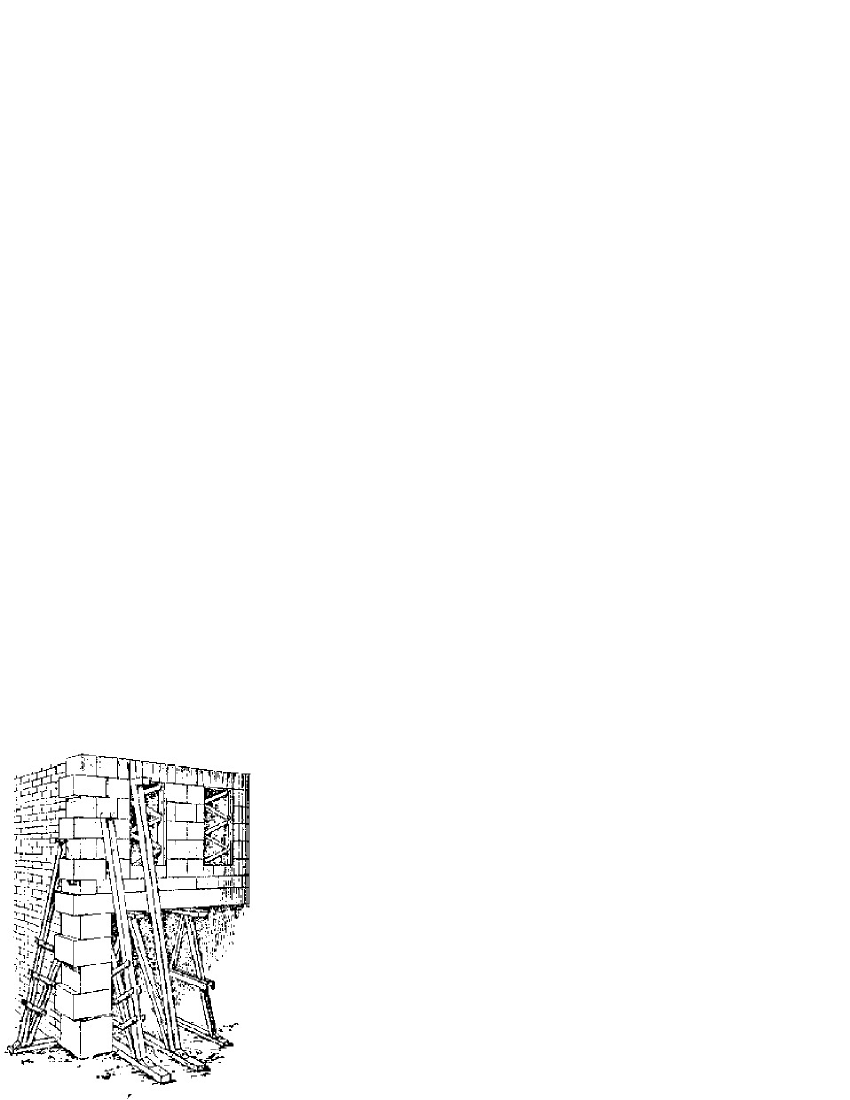
Figure 1: Shoring the edifice (reproduced from Fig. 813 in [17]).

The approach to quantum theory described in this paper by no means disproves the standard quantum mechanics. The founding fathers of quantum mechanics erected a remarkable edifice. But they began the construction with the second floor, the description of probabilities and means. Therefore, the stability of this edifice has required a large amount of shoring (see Fig. 1) in the form of a series of ”principles”: the superposition principle, the uncertainty principle, the principle of complementarity, the projection principle, the indistinguishability principle, and the principle of the absence of trajectories. All these principles appear rather artificial and are not easily amenable to physical interpretation. The main task of these principles is to justify the mathematical formalism of the standard quantum mechanics. True, this mathematical formalism has proved amazingly serendipitous, but this is not the case with its physical interpretation. It is not without reason that discussions of the physical interpretation of quantum mechanics still vividly proceed, although the term ”physical interpretation” itself seems quite strange. If quantum mechanics is a physical theory, then it must not need any physical interpretation. By using this term, we admit, be it willingly or not, that quantum mechanics is not a physical theory but a mathematical model. In this work, we have attempted to construct quantum mechanics just as a physical theory, based on experimental data.

The central point of the described approach is the introduction of the notion of an ”elementary state,” which is absent in the formalism of the standard quantum mechanics. This notion, on one hand, gives a clear mathematical counterpart of such a physical phenomenon as an individual experimental act. On the other hand, it allows using the well-developed formalism of classical logic and classical probability theory. It must be borne in mind here that although the references to the so-called quantum logic and quantum probability theory may be rather frequent, it has so far been impossible to give them the structure of a clear-cut complete theoretical scheme.

Based on the notion of an elementary state and using the classical probability theory, we can completely reproduce the mathematical formalism of the standard quantum mechanics and simultaneously show its applicability domain. This formalism applies to quantum ensembles. This is a very important type of ensemble but not the most general one by far. In particular, this formalism is not suitable for describing an individual event.

References

- [1]
- [2] von Neumann, Mathematische Grundlagen der Quantenmechanik, Verlag von Julius Springer, Berlin (1932).
- [3] D. A. Slavnov, Theor. Math. Phys., 142, 431 (2005).
- [4] J. Dixmier, Les C*-algebres et leurs representations, Gauthier-Villars, Paris (1969).
- [5] W. Rudin, Functional Analysis, McGraw-Hill, New York (1973).
- [6] S. Kochen and E. P. Specker, J. Math. Mech., 17, 59 (1967).
- [7] D. M. Greenberg, M. A. Horne, and A. Zeilinberg, Amer. J. Phys., 58, 1131 (1990).
- [8] A. N. Kolmogorov, Basic Notions of Probability Theory [in Russian] (2nd ed.), Nauka, Moscow (1974); English transl. prev. ed.: Foundations of the Theory of Probability, Chelsea, New York (1956).
- [9] D. A. Slavnov, Theor. Math. Phys., 136, 1273 (2003).
- [10] J. Neveu, Bases mathematiques du calcul des probabilites, Masson, Paris (1964).
- [11] J. F. Clauser, M. A. Horne, A. Shimony, and R. A. Holt, Phys. Rev. Lett., 23, 880 (1969).
- [12] J. S. Bell, Physics, 1, 195 (1965).
- [13] P. Jordan, Z. Phys., 80, 285 (1933).
- [14] G. G. Emch, Algebraic Methods in Statistical Mechanics and Quantum Field Theory, Wiley, New York (1972).
- [15] M. A. Neimark, Normed Rings [in Russian], Nauka, Moscow (1968); English transl., Wolters-Noordhoff, Groningen (1970).
- [16] M. Born, Z. Phys., 37, 863 (1926); 38, 803; 40, 167 (1927).
- [17] E. Barberot, Traite pratique de charpente, Librairie Polytechnique, Paris (1911).