Fractal Fidelity as a signature of Quantum Chaos

Abstract

We analyze the fidelity of a quantum simulation and we show that it displays fractal fluctuations iff the simulated dynamics is chaotic. This analysis allows us to investigate a given simulated dynamics without any prior knowledge. In the case of integrable dynamics, the appearance of fidelity fractal fluctuations is a signal of a highly corrupted simulation. We conjecture that fidelity fractal fluctuations are a signature of the appearance of quantum chaos. Our analysis can be realized already by a few qubit quantum processor.

Quantum signature of classical chaotic systems have been investigated widely in the last decades haake . Within the development of quantum information theory, a new interest on quantum chaotic systems arose motivated by the fact that they are interesting testbeds for quantum simulations. Indeed, the quantum simulation of quantum chaotic systems is possible and some efficient algorithms, with respect to known classical ones, have been found monta01 ; baker ; kickrot . Moreover, it has been shown that classical simulations of quantum chaotic systems are a difficult problem for classical computers due to the high presence of entanglement in the fully chaotic regime monta04 ; prosen . In a more general context the fidelity, the response to a Hamiltonian perturbation of a quantum system, has attracted a lot of attention since its introduction by Peres peres . Indeed it has been shown that the fidelity is of fundamental importance for the understanding of a system dynamics as it has been used to characterize the system integrability emerson , the feasibility of a quantum simulation monta01 ; monta02 and of quantum communication protocols dechiara ; romito ; bose , the quantum-classical transition casati0 , the signature of the chaos border tsallis , the effects of a bath zurek1 the environment induced decoherence zurek2 and the characterization of quantum phase transitions zanardi ; rossini ; cucchietti . It has also been shown that, under given conditions, the fidelity recall classical properties of chaotic systems as its decay rate is given by the classical Lyapunov exponent jacquod ; pastawski .

Differently from mentioned previous studies on the variance of fidelity fluctuations that characterize the system response (averaged over different initial conditions or an ensemble of different perturbations) starting from its complete knowledge varfluc , we approach the problem as for classical complex systems signal analysis. Suppose you have a black box you do not have a complete control on as, for example, a quantum computer with some given but unknown imperfections. Any system outcome, i.e. a result of a measurement, might be corrupted: in our example, the result of a quantum computation in presence of hardware imperfections. What might be learnt from such signal without completely characterize the system and/or without affording the cost of repetitions of the computation? In this scenario, we focus on the problem of finding a clear signature of chaos in a quantum systems: it is well known that in classical systems with mixed phase space, a fractal region arises at the border between integrable islands and the chaotic sea zaslavsky . These regions are known to be responsible for fractal conductance fluctuations as a function of a given parameter (Aharonov-Bohm flux) in open quantum systems in the semiclassical regime blumel and it has been shown that fractal fluctuations survive also in the deep quantum regime casati . Moreover, fractal properties of systems wave functions have been shown to appear under given conditions berry . Here we show that in a unitary evolution, in particular in a quantum computer running a quantum simulation in the presence of static imperfections, fidelity fractal fluctuations naturally arise as a function of time. We demonstrate that the fractal dimension of such fluctuations strikingly depends on the chaoticity of the dynamics: For integrable dynamics the fidelity dimension is integer while for chaotic dynamics it is fractional. This sensitivity is not restricted to a fully chaotic phase space: fidelity fractal fluctuations arise also in the chaotic regions of a mixed phase space. We establish this connection and we present two possible applications of this analisys. First of all it can be used as a testbed for a given quantum computer hardware: If running a simple (integrable) algorithm fractal fidelity fluctuations appears the hardware is not realible as quantum chaos has set in monta01 . Secondly, we present a method to investigate an unknown phase space (Husimi or Wigner function) of a general quantum system. Indeed the fractal dimension of the fidelity of a given quantum system can be used to extract the presence of a chaotic region in the system phase space. This is of fundamental importance as the simulation of quantum system is one of the most general application of quantum computation, however it is severely limited by the lack of methods, different from the complete wave function tomography, to extract information from the final wave function feynman ; casmon . In emerson , it has been shown that the average fidelity can be measured in a quantum processor; the sawtooth map algorithm has been recently performed on a three qubit NMR quantum processor cory1 and the fidelity experimentally measured on a three qubits quantum processor laflamme , thus, the proposed protocol is at the edge of present day technology.

This paper is structured as follows: in Section I we present the testbed for our findings, the Sawtooth Map and its simulation on a quantum computer in presence of imperfections. In Section II we introduce the tools to characterize the fidelity fractal fluctuations and we analyze the fidelity fractal dimension in different scenarios. Finally in Section III we introduce the phase space tomography via fidelity fractal dimension analysis and Section IV is devoted to our conclusions.

I Sawtooth Map

As an example of quantum system with complex dynamics we use the quantum sawtooth map. The correspondent classical map is characterized by a range of very different dynamics depending on system parameters varying from completely integrable, semi integrable to chaotic dynamics. It is defined by the equations

$${\cal T}:\left\{\begin{array}[]{ll}n_{i+1}&=n_{i}+k(\theta_{i}-\pi)\\ \\ \theta_{i+1}&=\theta_{i}+T\>n_{i+1}\end{array}\right.,$$ (1)

where $(n,\theta)$ are the conjugate action-variables $(0\leq\theta<2\pi)$, $k$ is the kick strength and $T$ the time between consecutives kicks. The dynamics is characterized by the parameter $K=kT$: it is chaotic for $K>0$, $K<-4$, integrable for $K=-3,-2,-1,0$ and with mixed phase space in the remaining regions cary . This map belongs to the kicked maps family, and it describes a system undergoing free evolution and subject to a kick every time $T$. The kick strength is proportional to $\theta^{2}$.

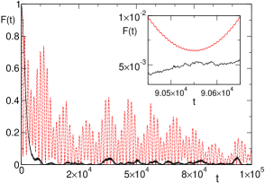
Figure 1: Fidelity as a function of time for integrable $K=-1$ (red, dashed) and chaotic regime $K=\sqrt{2}$ (black, full), with $\epsilon=10^{-4}$ and $n_{q}=8$. Inset: magnification of the behavior for long times.

After canonical quantization of the action angle variables, the correspondent quantum map is defined by the Floquet operator (time evolution operator for a period $T$)

$$\hat{U}=e^{-\frac{i}{2}T\hat{n}^{2}}e^{ik(\hat{\theta}-\pi)^{2}/2},$$ (2)

where $\hat{n}=-i\partial/\partial\theta$ and $\psi(\theta+2\pi)=\psi(\theta)$ (we set $\hbar=1$). The quantization rule is $[\hat{n},\hat{\theta}]=-i$.

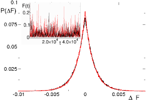
Figure 2: Fidelity (Inset) and distribution $P(\Delta F)$ of fidelity fluctuations $\Delta F=F_{i+1}-F_{i}$ for $n_{q}=6$, $\epsilon=10^{-3}$ for chaotic (black line) and integrable (red line) dynamics.

The map dynamics is still governed by the classical parameter $K$, but a key role is played also by $k=K/T$ which rules the quantum-classical transition ($k\to\infty$ is the classical limit, $T=2\pi/N$ with $N=2^{n_{q}}$ the Hilbert space size). In monta01 an efficient quantum algorithm has been introduced to simulate this map and the effects of static imperfections, present in any experimental apparatus, have been studied monta01 ; monta02 . The imperfections considered are both residual coupling between qubits and fluctuations of the single qubits level spacing. As the effects of the static imperfections are almost independent from their exact expression in terms of operators if there is a stronger leading dynamics (the quantum algorithm in our case) here we consider only the latter kind of error. The complete Hamiltonian that describes the hardware of the quantum computer is then

$$H=\sum_{i=1}^{n_{q}}(\Delta+\delta_{i})\sigma_{i}^{z}.$$ (3)

Here $\Delta$ is the mean qubit level spacing, $\delta_{i}$ are the fluctuations of the qubit level spacing taken randomly and uniformly in the interval $[-\epsilon;\epsilon]$ (constant in time) and $\sigma_{i}^{z}$ are the Pauli matrices. The Floquet operator in the presence of errors is then defined by the quantum gates needed to simulate a period of the map (2) with the action of the Hamiltonian (3). The Floquet eigenvalues and eigenvectors statistics have been studied in monta02 ; monta03 and it has been shown that eventually with growing imperfections strength the system ends to be chaotic regardless the simulated map dynamics monta02 . This crossover, is governed by the imperfections strength $\epsilon$ and it has been shown that in the case of integrable dynamics $\epsilon_{c}\propto n_{q}^{-5/2}$: this threshold for chaos appearance has been estimated from the breakdown of perturbation theory and confirmed numerically monta03 .

II Fractal fidelity fluctuations

We study the time fluctuations of the fidelity of a quantum computation. The fidelity is defined (for pure states) as

$$F(t)=|\left\langle\psi_{\epsilon}(t)\right||\psi(t)\rangle|^{2},$$ (4)

that is the overlap as a function of time of the wave function computed with the exact time evolution $\left|\psi(t)\right\rangle$ and the wave function in the presence of static imperfections $\left|\psi_{\epsilon}(t)\right\rangle$. The fidelity starts from one, it decays up to a saturation value and then oscillates around it after a transient time $t^{*}$.

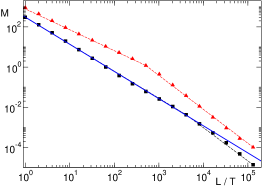
Figure 3: Results of the modified box counting algorithm for the fidelity of Fig.1: integrable (red triangles) and chaotic dynamics (squares). The blue full line is a guide for the eye proportional to $L^{1.36}$. Here $t^{*}\sim 10^{4}$. The resulting fractal dimensions are $D\sim 1.06$ for the integrable case and $D\sim 1.36$ for the chaotic dynamics.

In Fig. 1 we report two typical fidelities as a function of time for a chaotic and an integrable dynamics. Notice that the signals are not averaged over different static imperfections configuration: they could be the direct output of an “echo experiment”. We stress the fact that the two clear distinct behavior of the fidelity fluctuations shown in the inset of Fig. 1 reflect the presence, in the system classical limit, of a continuum set of typical frequencies of the system dynamics in the chaotic case differently from the discrete set of harmonics present in integrable systems. Even though in Fig. 1 the two curves appears pretty different and one could guess the underlaying behavior of the system under study, there are case where this is not the case. In Fig. 2 we show an example where not only the fidelity time dependence but also the distributions of the fluctuations are not distinguishable. In order to extract the information on the underlying dynamics one should use more sophisticated tools such as the study of the fractal dimension of the signal which detects, as for the classical cases, the presence of a “complex” set of typical frequencies of the system in the chaotic case and a “regular” spectrum in the integrable one.

The fractal dimension of the signal is measured by means of the modified box counting algorithm box1 . In the standard box counting algorithm the fractal dimension $D$ of the signal is obtained by covering the data with a grid of square boxes of size $L^{2}$.

Figure 4: Fractal dimension of the fidelity fluctuations $D$ as a function of Sawtooth Map parameter $K$, imperfections strength from $\epsilon=10^{-2}$ to $\epsilon=10^{-6}$ (from top to bottom) for $n_{q}=8$ averaged over $N_{R}<5$ different imperfections realizations.

The number $M(L)$ of boxes needed to cover the curve is recorded as a function of the box size $L$. The (fractal) dimension $D$ of the curve is then defined as

$$D=-\lim_{L\to 0}\log_{L}M(L).$$ (5)

One finds $D=1$ for a straight line, while $D=2$ for a periodic curve. Indeed, for times much larger than the period, a periodic curve covers uniformly a rectangular region. Any given value of $D$ in between of these integer values is a signal of the fractality of the curve. The modified algorithm of Ref. box1 follows the same lines but uses rectangular boxes of size $L\times\Delta_{i}$ ($\Delta_{i}$ is the largest excursion of the curve in the region $L$). Then, the number $M(L)=\frac{\sum_{i}\Delta_{i}}{L}$ is computed. For any curve that lays in a plane, a region of box lengths $L_{min}<L<L_{max}$ exists where $M\propto L^{D}$. Outside this region one either finds $D=1$ or $D=2$: The first equality ($D=1$) holds for $L<L_{min}$ and it is due to the coarse grain introduced by the discrete map time evolution. The second limit ($D=2$) is obtained for $L>L_{max}$ and it is due to the finite length of the analyzed time series. The boundaries $L_{min},L_{max}$ have to be chosen properly for any time series. In our analysis $L_{min}=T$ while $L_{max}\sim\epsilon^{-\alpha}$, where $\alpha$ increases with $n_{q}$.

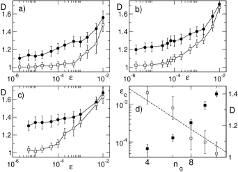
Figure 5: a,b,c) Fidelity fractal dimension $D$ as a function of imperfections strength $\epsilon$ averaged over different $K$ for integrable (white) and chaotic regime (black) for $n_{q}=6,8,10$.
d) Scaling of the critical imperfections strength $\epsilon_{c}\sim n_{q}^{-2.5}$ (white squares, left axis) and limiting fractal dimension $D(\epsilon=0)$ as a function of $n_{q}$ (black squares, right axis).

In Fig. 3 we report an example of this analysis for the long time behavior of the two signals of Fig. 1. We analyzed the time series starting from a given time $t^{*}$ to exclude the initial transient decay. In Fig. 4 we summarize our results reporting the fractal dimension of the fidelity for different values of $K$ spanning a wide range of different dynamics (excluding mixed phase space) and for different $\epsilon$ values. Again, the signature of chaotic dynamics is striking. Notice that in the chaotic region the fractal dimension of the fidelity fluctuations appears to be $K$ independent. Thus, we average over different $K$ in both regimes (integrable and chaotic) to study the dependence of $D$ as a function of the number of qubits and the imperfections strength. In Fig. 5 (a, b, c) we show the extended analysis of the fractal dimension of the fidelity fluctuations as a function of the number of qubits in the quantum hardware and imperfections strength for the two distinct dynamics. The difference is striking: for chaotic dynamics the dimension is fractal for any value of the imperfections strength. On the contrary, for integrable dynamics the dimension of the fidelity fluctuations is one until a critical value of the imperfections strength $\epsilon_{c}$. In Fig. 5 d, we show the scaling of $\epsilon_{c}$ as a function of the number of qubits in the system. Although the scaling is on a very small range of parameter, it scales as the critical value for which the integrable dynamics became chaotic due to the imperfections effect monta03 . It is then clear, that above $\epsilon_{c}$ the system is chaotic due to the imperfections and regardless of the map dynamics: this transition is reflected by the appearance of fractal fluctuations. Increasing further the imperfections strength eventually the fidelity loses all the information regarding the underlying dynamics and indeed the fractal dimensions related to the two distinct dynamics are equal. The error bars are due to the sensitivity of the results to the choice of $L_{min}$ and $L_{max}$. In Fig. 5 d we also show the scaling of the fractal dimension $D(n)$ as a function of the number of qubits in the limit $\epsilon\to 0$ for the chaotic regime. The signature of quantum chaos is again striking and the difference between the two regimes grows with the system size.

Notice that this analysis can be performed already with a few qubits quantum computer (see Fig. 5 a). The biggest obstacle to a possible implementation is the length of the time series and the correspondent necessary long coherent times. However, we checked that already with boxes of sizes $L\sim 10$ in a time series of few hundred points, the different scalings in the two cases are clearly visible. It is also possible, for small $\epsilon$, to perform the same analysis on the initial part of the fidelity after subtracting the average decay (data not shown). Although this procedure might suffer from errors due to fitting procedure of the average behavior, it paves the way to an efficient measurement of the fractal dimension of the fidelity fluctuations.

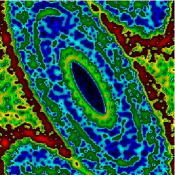
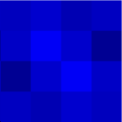
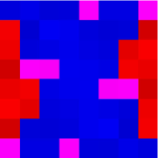
Figure 6: (Color online) Upper left panel: Husimi function of the Sawtooth Map phase space $(\theta,n)$ for an initial gaussian condition inside the chaotic sea ($D=1.34$) for $\epsilon=2\cdot 10^{-5}$, $n_{q}=10$, $t=2^{14}$. Other panels: Phase space tomography with different resolutions. Fractal dimension of the fidelity fluctuations as a function of the initial condition ($4\times 4,8\times 8$ and $16\times 16$) for $n_{q}=10$ and $\epsilon=2\cdot 10^{-5}$, $N_{R}=1$. The color code goes from blue, yellow to red to represent higher values of probability or fractal dimension.

III Phase space Tomography

Finally, we concentrate on the fidelity fluctuations as a function of the initial condition in the case of mixed phase space. In the upper left panel of Fig.6 we report the Husimi function of the phase space of the Sawtooth Map for $K=-2.1$, $T=2\pi/N$ where the chaotic sea and the integrable islands are clearly visible husimi ; monta01 . The initial conditions is a gaussian packet which satisfy the minimal indetermination Heisenberg condition centered inside the chaotic sea. In the lower panels of Fig.6 we show the result of the phase space tomography with the proposed method with a discretization of $4\times 4$, $8\times 8$ and $16\times 16$ initial conditions. For every initial condition, a gaussian packet centered in $(n_{0},\theta_{0})$, we computed the fractal dimension of the fidelity fluctuations $D(n_{0},\theta_{0})$ and plotted the resulting contour plot from $D=1$ (black) to $D=D_{max}$ (red). We found again that the dimension of the fidelity depends on the underlying dynamics: a fractional dimension is found for the chaotic sea while it is integer when the dynamics lies inside the integrable islands. The result is a partition of the phase space in chaotic and integrable regions which can be refined increasing the number of different initial conditions (notice that the resolution of the Husimi is of the order of $N^{2}=2^{20}$ points). Thus, this analysis can be used as a tool to scan an unknown phase space of a given Hamiltonian dynamics to discern between integrable and chaotic phase space regions.

IV Conclusions

In conclusion, the fidelity time fluctuations are a signature of quantum chaotic dynamics. They reflect, as for classically chaotic signals, the presence of an “almost-continuum” of frequencies in the system dynamics compared to the “discrete” set of typical frequencies of integrable systems. A similar behavior has been already observed in the context of quantum communication in spin chains dechiara . We propose this kind of analysis to investigate an unknown phase space of a complex quantum system and to test the effects of static imperfections of quantum hardware. We stress that the sensitivity of the fidelity fluctuations of a simulated system dynamics is valid also in the limit of imperfections strength going to zero, i.e. they will be present in any experimental quantum hardware in case of chaotic or mixed phase space dynamics. Similar results are likely to be found in presence of time dependent imperfections (errors) in the quantum system along the lines of facchi .

We thank R. Fazio, G. Benenti and D. Frustaglia for useful discussions. This work has been supported by the “Quantum Information Program” of Centro De Giorgi of Scuola Normale Superiore and by EUROSQIP. SM acknowledges support from the Alexander Von Humboldt Foundation.

References

- (1) F.Haake, “Quantum Signature of Chaos”, Springer Verlag (2001).
- (2) G. Benenti, G. Casati, S. Montangero and D.L. Shepelyansky Phys. Rev. Lett 87, 227901 (2001).
- (3) T.Brun, R.Schack, Phys.Rev. A 59 2649 (1999).
- (4) B.Levi, B.Georgeot, D.L. Shepelyansky, Phys. Rev. E 67 046220 (2003).
- (5) S.Montangero, Phys. Rev. A 70, 032311 (2004).
- (6) T. Prosen, M Znidaric, arXiv:quant-ph/0608057.
- (7) A. Peres, Phys. Rev. A 30, 1610 (1984).
- (8) J.Emerson, Y.Weinstein, S.Lloyd, and D.G. Cory, Phys. Rev. Lett. 89, 284102 (2002).
- (9) G. Benenti, G. Casati, S. Montangero and D.L. Shepelyansky, Eur. Phys. J. D 22, 285 (2003).
- (10) G. De Chiara, D. Rossini, S. Montangero and R. Fazio, Phys. Rev. A 72, 012323 (2005).
- (11) A. Romito, R. Fazio and C. Bruder, Phys. Rev. B 71 100501 (2005).
- (12) S. Bose, Phys. Rev. Lett. 91, 207901 (2003).
- (13) G.Benenti and G. Casati, Phys. Rev. E 65, 066205 (2002).
- (14) Y. Weinstein, S. Lloyd and C. Tsallis, Phys. Rev. Lett. 89 214101 (2002)
- (15) F.M.Cucchietti, J.P. Paz, and W.H.Zurek, Phys. Rev. A 72 052113 (2005).
- (16) F.M. Cucchietti, D.A.R. Dalvit, J.P. Paz, W.H. Zurek, Phys. Rev. Lett. 91 210403 (2003).
- (17) P. Zanardi and N. Paunković, Phys. Rev. E 74 031123 (2006)
- (18) D. Rossini, T. Calarco, V. Giovannetti, S. Montangero and R. Fazio, J. Phys. A: Math. Theor. 40 8033 (2007).
- (19) F.M. Cucchietti arXiv:quant-ph/0609202.
- (20) P. Jacquod, P.G. Silvestrov and C.W.J. Beenakker, Phys. Rev. E 64 055203 (2001).
- (21) R. A. Jalabert and H. M. Pastawski, Phys. Rev. Lett. 86, 2490 (2001).
- (22) G.M. Zaslavsky, “Physics of chaos in hamiltonian systems”, Imperial College Press, (1998).
- (23) R.Blümel and U.Smilansky, Phys. Rev. Lett. 60, 477 (1988).
- (24) G. Benenti, G. Casati, I. Guarneri and M. Terraneo, Phys. Rev. Lett. 87 014101 (2001).
- (25) M.V. Berry, J. Phys. A 29 (1996) 6617.
- (26) T. Prosen, M. Znidaric J.Phys. A 1455, 35 (2002); C. Petitjean, P. Jacquod Phys. Rev. E 71, 036223 (2005).
- (27) R.P. Feynman, Int. J. Theor. Phys. 21, 467 (1982)
- (28) G.Casati, S.Montangero, “Decoherence and Entropy in Complex Systems”, ed. H.-T. Elze, Lect. Notes in Phys. 633, 341 (Springer, Berlin, 2004).
- (29) M.K. Henry, J. Emerson, R. Martinez and D.G. Cory, Phys. Rev A 74 062317 (2006).
- (30) A.C. Ryan, J. Emerson, D. Poulin, C. Negrevergne,R. Laflamme, Phys. Rev. Lett., 95, 250502 (2005).
- (31) J. Cary, J.D. Meiss, Phys. Rev. A 24, 2664 (1981).
- (32) G. Benenti, G. Casati, S. Montangero and D.L. Shepelyansky, Eur. Phys. J. D 20, 293 (2002).
- (33) A.S. Sachrajda, R. Ketzmerick, C. Gould, Y. Feng, P.J. Kelly, A. Delage, and Z. Wasilewski, Phys. Rev. Lett 80 1948 (1998).
- (34) K. Husimi, Proc. Phys. Math. Soc. Jpn. 22, 264 (1940).
- (35) P. Facchi, S. Montangero, R. Fazio and S. Pascazio, Phys. Rev. A (R) 71, 060306 (2005).