Lifshitz Interaction between Dielectric Bodies of Arbitrary Geometry

Abstract

A formulation is developed for the calculation of the electromagnetic–fluctuation forces for dielectric objects of arbitrary geometry at small separations, as a perturbative expansion in the dielectric contrast. The resulting Lifshitz energy automatically takes on the form of a series expansion of the different many-body contributions. The formulation has the advantage that the divergent contributions can be readily determined and subtracted off, and thus makes a convenient scheme for realistic numerical calculations, which could be useful in designing nano-scale mechanical devices.

Since the pioneering work of van der Waals in 1873—which revealed that condensation of gases is not possible unless an attractive interaction is at work in matter—and the explanation of this interaction by London in 1930 in terms of the correlation between quantum fluctuations of atoms and molecules Israelachvili92 , we have been witnessing a surge of interest in exploring the physical implications of such fluctuation–induced interactions Kardar99 ; Bordag+01 . The case of two parallel plates made of perfect conductors tackled by Casimir Casimir48 and the subsequent generalization to the case of dielectric materials by Lifshitz Lifshitz made important contributions to our understanding of the macroscopic manifestations of these interactions. Relevant experimental studies, which were ongoing alongside with the theoretical developments Israelachvili92 , culminated recently with high precision quantitative verifications of the Casimir force Lamoreaux97 ; MR98 ; CAKBC2001 ; Bressi02 .

The advent of nanotechnology in recent years has added to the interest in electromagnetic–fluctuation interactions as they become dominant at nanoscale Srivastava+85 , and quantitative knowledge of them appears to be necessary in designing nano-machines to avoid unwanted effects such as stiction Serry+95 ; Buks+01 . Moreover, one could even make use of these interactions, e.g. the normal Casimir force between a flat plate and a sphere CAKBC2001 ; chanosc or the lateral Casimir force between two corrugated surfaces GK ; Chen+02 , in designing novel actuation schemes in microelectromechanical systems (MEMS). It thus seems desirable to be able to calculate the electromagnetic–fluctuation forces for a given assortment of dielectric and metallic objects in a certain configuration.

This, however, appears to be a nontrivial task due a number of subtleties involved. Casimir forces are known to depend in a nontrivial way on the geometry of the objects RM99 , and the theoretical schemes that have so far been developed to study this effect are only applicable to perfect conductors GK ; RM99 ; Balian ; EHGK ; Jaffe ; Emig . On the other hand, Lifshitz has pointed out that the electromagnetic–fluctuation force between two boundaries is dominated by the dielectric properties of the media in the frequency that is set by the separation between them Lifshitz . This means that when these forces are most relevant, i.e. at length scales lower than $100$ nm that is of the order the plasma wavelengths of most good metals, the perfect conductor assumption in the calculation of the Casimir force breaks down. Finally, the dependence of the divergent contributions to the Casimir energy—that should be removed in a carefully regularized formulation—on the geometry of the boundaries is not well characterized, and this makes it difficult to develop systematic numerical schemes of calculations.

The fact that the Lifshitz interactions at small separations effectively involve dielectric constants at relatively high-frequencies suggests that a strategy based on expansion in dielectric contrast could act as a useful complementary approach to the existing formulations. Here, we have developed a path integral formulation for calculating the Lifshitz energy for dielectric bodies of arbitrary geometry, as an expansion in powers of the variations in the dielectric constant in space (see Fig. 1a). The result effectively takes on the form of an expansion in many-body interactions with a fundamental tensorial kernel that reflects the nature of the electromagnetic fluctuations, with explicit expressions for all of the terms in the series. It has the advantage that the divergent contributions in the series are manifest and can be subtracted off systematically, which makes it very suitable for numerical calculations.

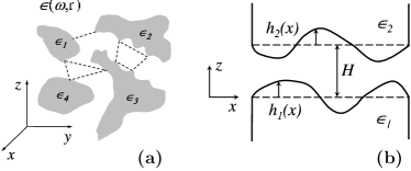
Figure 1: Schematics of (a) the dielectric function profile, and the many-body contributions to the electromagnetic–fluctuation forces, and (b) the two semi-infinite dielectric bodies with irregular surfaces.

We start with the action integral for the electromagnetic field in a matter with dielectric constant $\epsilon$, i.e. ${\cal S}_{\rm m}=\frac{1}{8\pi}\int dtd^{3}{\bf x}\left[\epsilon{\bf E}^{2}-{\bf B}^{2}\right]$, where standard expressions for the electric field ${\bf E}=-\frac{1}{c}\partial_{t}{\bf A}-\nabla\phi$ and the magnetic field ${\bf B}=\nabla\times{\bf A}$ are assumed in terms of the potentials $\phi$ and ${\bf A}$. To perform the quantization, we need to express the action in terms of the potentials and break the gauge invariance by choosing a particular gauge. Using the temporal gauge, $\phi=0$, we can write the action integral as ${\cal S}_{\rm m}=\frac{1}{8\pi}\int\frac{d\omega}{2\pi}\int d^{3}{\bf r}\;A_{i}(-\omega,{{\bf r}})[\epsilon(\omega,{\bf r})(\omega/c)^{2}\delta_{ij}+\partial_{k}\partial_{k}\delta_{ij}-\partial_{i}\partial_{j}]A_{j}(\omega,{{\bf r}}),$ where summation over repeated indices is assumed. In this expression, $\epsilon(\omega,{\bf r})$ is the frequency dependent dielectric function of the medium, which could represent any spatial arrangement of dielectric objects of arbitrary shapes, as depicted in Fig. 1a.

The quantization can now be performed by using the path integral method, which is facilitated if a Wick rotation is performed in the frequency domain. This renders the action integral “Euclidean” and we can find the partition function ${\cal Z}=\int{\cal D}A_{i}\;\exp\left(-{\cal S}_{\rm m}^{\rm Euclidean}/\hbar\right)$, and the Lifshitz energy $E=-\frac{\hbar}{T}\ln{\cal Z}$, where $T$ is a long observation time. The calculation yields

$$E=\hbar\int_{0}^{\infty}\frac{d\zeta}{2\pi}\;\log\det\left[{\cal K}_{ij}(\zeta;{\bf r},{\bf r}^{\prime})\right],$$ (1)

where ${\cal K}_{ij}=\left[(\zeta/c)^{2}\epsilon(i\zeta,{\bf r})\delta_{ij}+\partial_{i}\partial_{j}-\partial_{k}\partial_{k}\delta_{ij}\right]\delta^{3}({\bf r}-{\bf r}^{\prime}).$ Writing $\epsilon(i\zeta,{\bf r})=1+\delta\epsilon(i\zeta,{\bf r})$, we can decompose the kernel ${\cal K}_{ij}$ into a diagonal part that corresponds to the empty space and a perturbation that entails the dielectric inhomogeneity profile. In Fourier space, this reads ${\cal K}_{ij}(\zeta;{\bf q},{\bf q}^{\prime})={\cal K}_{0,ij}(\zeta,{\bf q})(2\pi)^{3}\delta^{3}({\bf q}+{\bf q}^{\prime})+\delta{\cal K}_{ij}(\zeta;{\bf q},{\bf q}^{\prime})$, where ${\cal K}_{0,ij}(\zeta,{\bf q})=(\zeta/c)^{2}\delta_{ij}+q^{2}\delta_{ij}-q_{i}q_{j}$ and $\delta{\cal K}_{ij}(\zeta;{\bf q},{\bf q}^{\prime})=(\zeta/c)^{2}\delta_{ij}\delta\tilde{\epsilon}(i\zeta,{\bf q}+{\bf q}^{\prime})$. We can now recast the expression for the Lifshitz energy into a perturbative series by using ${\rm tr}\ln[{\cal K}]={\rm tr}\ln[{\cal K}_{0}]+\sum_{n=1}^{\infty}\frac{(-1)^{n-1}}{n}\;{\rm tr}[({\cal K}_{0}^{-1}\delta{\cal K})^{n}]$, where $\displaystyle{\cal K}_{0,ij}^{-1}(\zeta,{\bf q})=\frac{(\zeta/c)^{2}\delta_{ij}+q_{i}q_{j}}{(\zeta/c)^{2}[\left(\zeta/c)^{2}+q^{2}\right]}.$ Using these definitions, one can write the explicit form for the trace as

$${\rm tr}[({\cal K}_{0}^{-1}\delta{\cal K})^{n}]=\int\frac{d^{3}{\bf q}^{(1)}}{(2\pi)^{3}}\cdots\frac{d^{3}{\bf q}^{(n)}}{(2\pi)^{3}}$$

$$\hskip 14.22636pt\times\frac{[(\zeta/c)^{2}\delta_{i_{1}i_{2}}+q_{i_{1}}^{(1)}q_{i_{2}}^{(1)}]\cdots[(\zeta/c)^{2}\delta_{i_{n}i_{1}}+q_{i_{n}}^{(n)}q_{i_{1}}^{(n)}]}{[(\zeta/c)^{2}+q^{(1)2}]\cdots[(\zeta/c)^{2}+q^{(n)2}]}$$

$$\hskip 14.22636pt\times\;\delta\tilde{\epsilon}(i\zeta,-{\bf q}^{(1)}+{\bf q}^{(2)})\cdots\;\delta\tilde{\epsilon}(i\zeta,-{\bf q}^{(n)}+{\bf q}^{(1)}),$$ (2)

which involves the geometric information about the arrangement of the dielectric objects through the Fourier transform of the dielectric function profile. Transforming back the expression in Eq. (2) into real space, we find the following series for the Lifshitz energy of any heterogeneous dielectric medium

$$E = \hbar\int_{0}^{\infty}\frac{d\zeta}{2\pi}\;\sum_{n=1}^{\infty}\frac{(-1)^{n-1}}{n}\;\int d^{3}{\bf r}_{1}\cdots d^{3}{\bf r}_{n}$$ (3)

$$\times\;{\cal G}^{\zeta}_{i_{1}i_{2}}({\bf r}_{1}-{\bf r}_{2})\cdots\;{\cal G}^{\zeta}_{i_{n}i_{1}}({\bf r}_{n}-{\bf r}_{1})$$

$$\times\;\delta\epsilon(i\zeta,{\bf r}_{1})\cdots\;\delta\epsilon(i\zeta,{\bf r}_{n}),$$

where the Green’s function associated with the electromagnetic fluctuations is defined as

$${\cal G}^{\zeta}_{ij}({\bf r}) = \frac{(\zeta/c)^{2}}{4\pi}\frac{{\rm e}^{-\zeta r/c}}{r}\left[\delta_{ij}\left(1+\frac{c}{\zeta r}+\frac{c^{2}}{\zeta^{2}r^{2}}\right)\right.$$ (4)

$$\left.-\frac{r_{i}r_{j}}{r^{2}}\left(1+3\frac{c}{\zeta r}+3\frac{c^{2}}{\zeta^{2}r^{2}}\right)\right]+\frac{1}{3}\delta_{ij}\delta^{3}({\bf r}).$$

This result has a number of interesting characteristics. First, it appears that an expansion in powers of $\delta\epsilon$ automatically turns into a summation of integrated contributions of $n$-body interactions. Moreover, all of the $n$-body interaction terms have simple expressions in terms of a single fundamental kernel ${\cal G}^{\zeta}_{ij}({\bf r})$ that mediates the two-body part of the interaction. This kernel is tensorial, and has the structure of the electric field of a radiating dipole in imaginary frequency Jackson . It has, in fact, been introduced some time ago in connection with van der Waals interactions Green . Finally, the result has a closed form expression for the Lifshitz energy for any geometrical arrangement of dielectric bodies in terms of quadratures.

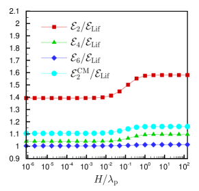
Figure 2: Comparison of the expansion in Eq. (3) up to the second, fourth, and sixth order, as well as the Clausius-Mossotti approximation, with the exact Lifshitz result for a pair of parallel semi-infinite dielectrics, as a function of their separation $H$ in units of the plasma wavelength $\lambda_{\rm p}$. The dielectric constant of both objects is chosen as $\epsilon(i\zeta)=1+\omega_{\rm p}^{2}/(\omega_{0}^{2}+\zeta^{2})$ with $\omega_{0}^{2}=2\;\omega_{\rm p}^{2}$.

To examine the convergence property of the above series, we can take a specific example for which the exact result is known, and compare it with what we find from the first few terms in Eq. (3). We consider the case of two identical semi-infinite dielectric objects that are placed parallel to each other at a separation $H$, for which the exact expression for energy per unit area is known to be ${\cal E}_{\rm Lif}=\frac{\hbar}{4\pi^{2}c^{2}}\int_{0}^{\infty}d\zeta\;\zeta^{2}\int_{1}^{\infty}dp\;p\left\{\ln\left[1-\frac{(s-p)^{2}}{(s+p)^{2}}{\rm e}^{-2p\zeta H/c}\right]\right.+\left.\ln\left[1-\frac{(s-p\epsilon)^{2}}{(s+p\epsilon)^{2}}{\rm e}^{-2p\zeta H/c}\right]\right\},$ where $s=\sqrt{\epsilon-1+p^{2}}$ Lifshitz . To calculate the energies, we have assumed a simple form $\displaystyle\epsilon(i\zeta)=1+\frac{\omega_{\rm p}^{2}}{\omega_{0}^{2}+\gamma\zeta+\zeta^{2}}$ for the dielectric constant, where $\omega_{\rm p}$ represents the plasma frequency, from which the plasma wavelength $\lambda_{\rm p}=2\pi c/\omega_{\rm p}$ can be extracted. In Fig. 2, the ratio between the energy as calculated from Eq. (3) up to the second, fourth, and sixth order and the exact Lifshitz result is shown as a function of the separation in units of the plasma wavelength for $\omega_{0}^{2}=2\;\omega_{\rm p}^{2}$ and $\gamma=0$, which corresponds to a dielectric with $\epsilon(0)=1.5$. The results clearly show a crossover between two asymptotic regimes near $H\approx\lambda_{\rm p}/(2\pi)$ note1 . The series appears to be rapidly convergent so long as $\delta\epsilon(0)<1$, and the convergence is considerably more efficient for $H<\lambda_{\rm p}/(2\pi)$ [as compared to $H>\lambda_{\rm p}/(2\pi)$], especially for $\delta\epsilon(0)\lesssim 1$. The damping constant $\gamma$ appears to have very little effect on the Lifshitz energy for dielectrics (i.e. when $\omega_{0}\neq 0$). The results presented in Fig. 2, for example, do not change appreciably for nonvanishing damping constants of up to $\gamma=0.1\;\omega_{\rm p}$.

It is quite well known that any calculation of the Casimir or Lifshitz energy encounters a variety of divergent contributions that are very difficult to characterize. For example, it is not clear how these divergent terms depend on the geometry of the system, so that they could be identified in a simple geometry and done away with in a systematic way for slightly deformed boundaries, in the calculations that involve perturbation in the geometry of the objects GK ; EHGK . While the present formulation also suffers from this deficiency, in the sense that the expression in Eq. (3) involves divergent contributions, the fact that the expressions for the various terms in the series are known a priori allows for systematic identification of these contributions and thus their systematic cancelation. For example, one can show that putting $1$ instead of the fraction in the second line of Eq. (2) yields a singular contribution of the form $E_{\rm sing.}=\hbar\int_{0}^{\infty}\frac{d\zeta}{2\pi}\int d^{3}{\bf r}\;\ln\left[\epsilon(i\zeta,{\bf r})\right]\int\frac{d^{3}{\bf q}}{(2\pi)^{3}},$ which could be subtracted off systematically (i.e. at every order $n$ in the series expansion) for any geometry and dielectric configuration.

Let us now focus our attention on the specific arrangement shown in Fig. 1b, where two semi-infinite dielectric bodies with irregularly shaped boundaries are placed nearly parallel to each other at a mean separation $H$. We can write down the dielectric function profile as

$$\epsilon(i\zeta,{\bf r})=\left\{\begin{array}[]{ll}\epsilon_{2}(i\zeta),&\;H+h_{2}({\bf x})\leq z<+\infty,\\ \\ 1,&\;h_{1}({\bf x})<z<H+h_{2}({\bf x}),\\ \\ \epsilon_{1}(i\zeta),&\;-\infty<z\leq h_{1}({\bf x}),\end{array}\right.$$ (5)

and the corresponding Fourier transform as $\delta\tilde{\epsilon}(i\zeta,{\bf q})=\frac{i}{q_{z}}\int d^{2}{\bf x}\;{\rm e}^{i{\bf q}_{\perp}\cdot{\bf x}}[\delta\epsilon_{2}\;{\rm e}^{iq_{z}\left[H+h_{2}({\bf x})\right]}-\delta\epsilon_{1}\;{\rm e}^{iq_{z}h_{1}({\bf x})}].$ When the separation of the surfaces is smaller than the plasma wavelengths of the two dielectric media, and $\delta\epsilon_{1}$ and $\delta\epsilon_{2}$ are small compared to unity, the leading contribution in Eq. (3) comes from the second order term. Putting in the dielectric function profile, we find

$$E_{2} = -\frac{\hbar}{128\pi^{3}c^{4}}\int_{0}^{\infty}d\zeta\;\zeta^{4}\;\delta\epsilon_{1}(i\zeta)\delta\epsilon_{2}(i\zeta)$$

$$\times \int d^{2}{\bf x}d^{2}{\bf x}^{\prime}\;{\cal W}\left(\frac{\zeta}{c}[{\bf x}-{\bf x}^{\prime}],\frac{\zeta}{c}[H+h_{2}({\bf x})-h_{1}({\bf x}^{\prime})]\right),$$

where

$${\cal W}({\bf y},h)=8\;\Gamma\left(0,2\sqrt{y^{2}+h^{2}}\right)+\int_{1}^{\infty}\frac{ds}{s^{3/2}}\;{\rm e}^{-2\sqrt{y^{2}+h^{2}s}}$$

$$\times\left[\frac{3}{(y^{2}+h^{2}s)^{2}}+\frac{6}{(y^{2}+h^{2}s)^{3/2}}+\frac{4\;(1-h^{2}s)}{(y^{2}+h^{2}s)}\right],$$

(7)

with the incomplete gamma function defined as $\Gamma(a,z)=\int_{z}^{\infty}dt\;t^{a-1}\;{\rm e}^{-t}$. Note that at this order, the Lifshitz energy is pairwise additive. In the above result, we have kept the frequency dependence of the dielectric functions as well as the geometry of the boundaries arbitrary for generality of the presentation Barton . The expression in Eq. (LABEL:E-2-1) can be considerably simplified for $h_{1}({\bf x})=0$:

$$\left.E_{2}\right|_{h_{1}({\bf x})=0}=\int d^{2}{\bf x}\;{\cal E}_{2}\left(H+h_{2}({\bf x})\right),$$ (8)

in terms of the original Lifshitz result for the energy per unit area of flat boundaries Lifshitz

$${\cal E}_{2}(H)=-\frac{\hbar}{64\pi^{2}c^{2}}\int_{0}^{\infty}d\zeta\;\zeta^{2}\;\delta\epsilon_{1}(i\zeta)\delta\epsilon_{2}(i\zeta){\cal L}\left(\frac{\zeta H}{c}\right),$$ (9)

with ${\cal L}(u)=4(u^{2}-1)E_{1}(2u)+\frac{{\rm e}^{-2u}}{u^{2}}(1+2u+u^{2}-2u^{3}),$ and the exponential integral function defined as $E_{n}(z)=\int_{1}^{\infty}dt\;{\rm e}^{-zt}/t^{n}$. This simplification is a general feature of pairwise additive interactions, as shown in Ref. EHGK .

The pairwise summation approximation is widely used in the literature not only for dielectric materials at close separations but also for perfect conductors at arbitrary separations. We can use the present formulation to shed some light on the nature of this approximation, and make assessment on what is not included. Going back to Eq. (4), we note that the Green’s function ${\cal G}^{\zeta}_{ij}({\bf r})$ is decomposed into a long-ranged kernel, and a “contact” part in the form of $\frac{1}{3}\delta_{ij}\delta^{3}({\bf r})$. A systematic pairwise summation approximation then amounts to keeping two of the ${\cal G}^{\zeta}_{ij}$’s in its full form and approximating the rest of them by their contact-contribution, in each term of the series in Eq. (3). Considering the different ways of doing this and keeping track of the corresponding combinatorial prefactors, one can then sum up the entire series and find a closed form expression for the Lifshitz energy between objects of arbitrary shapes in the pairwise summation approximation. The result will be identical to Eq. (LABEL:E-2-1) except for the replacement $\delta\epsilon_{i}\to\frac{\delta\epsilon_{i}}{1+(\delta\epsilon_{i}/3)}=3\left(\frac{\epsilon_{i}-1}{\epsilon_{i}+2}\right).$ The combination reminds us of the Clausius-Mossotti equation for molecular polarizability, which is well known to be valid only for dilute materials such as gases Jackson . This approximation allows us to calculate the energy for perfect conductors, and we can use the example of two flat and parallel perfect conductors, for which the exact result is known to be ${\cal E}^{c}_{\rm exact}=-\frac{\pi^{2}}{720}\frac{\hbar c}{H^{3}}$, to assess its validity. Letting $\epsilon_{1},\epsilon_{2}\to\infty$, we find ${\cal E}^{c}_{\rm PWS}=-\frac{69}{640\pi^{2}}\frac{\hbar c}{H^{3}}$, which compares to the exact result as $\frac{{\cal E}^{c}_{\rm PWS}}{{\cal E}^{c}_{\rm exact}}=\frac{621}{8\pi^{4}}\simeq 0.797.$ While this ratio varies with geometry, it gives us an estimate of typical errors that are involved in the calculations based on pairwise summation approximation. We also note that any attempt in going beyond this approximation should include the tensorial structure involved in Eq. (3), and for example, an ad hoc augmentation by introduction of scalar three-body interactions etc. will not be justified in light of our present scheme. The Clausius-Mossotti approximation appears to give comparatively better results for the case of dielectrics, as can be seen from the example in Fig. 2.

The formulation presented here could also be applied to the case of magnetic materials mag . For a medium that is described by the dielectric function profile $\epsilon(\omega,{\bf r})$ and the magnetic permeability profile $\mu(\omega,{\bf r})$, we should replace the kernel in Eq. (1) by ${\cal K}_{ij}(\zeta;{\bf r},{\bf r}^{\prime})=[(\zeta/c)^{2}\epsilon(i\zeta,{\bf r})\delta_{ij}+\partial_{i}\frac{1}{\mu(i\zeta,{\bf r})}\partial_{j}-\partial_{k}\frac{1}{\mu(i\zeta,{\bf r})}\partial_{k}\delta_{ij}]\delta^{3}({\bf r}-{\bf r}^{\prime}),$ and the rest of the procedure follows closely. Generalization to the case of finite temperatures by discretizing the frequency is also straightforward.

In conclusion, we have presented a path integral formulation for the calculation of the Lifshitz energy for dielectric materials of arbitrary shape, as a series expansion in the dielectric contrast. The expansion converges very rapidly for dielectric objects that are at separations considerably smaller than their corresponding plasma wavelengths, and is expected to work perfectly for surfaces at nanometric separations. The results presented here could be applicable for the calculation of electromagnetic–fluctuation forces that are involved in nano-mechanical devices.

It is a great pleasure to acknowledge fruitful discussions with M.A. Charsooghi, T. Emig, A. Hanke, M. Kardar, R. Matloob, M.F. Miri, and F. Mohammad-Rafiee.

References

- (1) J.N. Israelachvili, Intermolecular and Surface Forces (Academic, London, 1992).
- (2) M. Kardar and R. Golestanian, Rev. Mod. Phys. 71, 1233 (1999).
- (3) M. Bordag, U. Mohideen, V.M. Mostepanenko, Phys. Rep. 353, 1 (2001).
- (4) H.B.G. Casimir, Proc. K. Ned. Akad. Wet. 51, 793 (1948).
- (5) E.M. Lifshitz, Sov. Phys. JETP 2, 73 (1956); I.E. Dzyaloshinskii, E.M. Lifshitz, and L.P. Pitaevskii, Adv. Phys. 10, 165 (1961).
- (6) S.K. Lamoreaux, Phys. Rev. Lett. 78, 5 (1997); 81, 5475(E) (1998); Phys. Rev. A 59, R3149 (1999).
- (7) U. Mohideen and A. Roy, Phys. Rev. Lett. 81, 4549 (1998); B.W. Harris, F. Chen, and U. Mohideen, Phys. Rev. A 62, 052109 (2000).
- (8) H.B. Chan, V.A. Aksyuk, R.N. Kleiman, D.J. Bishop, and F. Capasso, Science 291, 1941 (2001).
- (9) G. Bressi, G. Carugno, R. Onofrio, and G. Ruoso, Phys. Rev. Lett. 88, 041804 (2002).
- (10) Y. Srivastava, A. Widom, and M.H. Friedman, Phys. Rev. Lett. 55, 2246 (1985); M.A. Stroscio, Phys. Rev. Lett. 56, 2107 (1986).
- (11) F.M. Serry, D. Walliser, and G.J. Maclay, J. Microelectromech. Syst. 4, 193 (1995); J. Appl. Phys. 84, 2501 (1998).
- (12) E. Buks and M.L. Roukes, Phys. Rev. B 63, 033402 (2001); Nature 419, 119 (2002).
- (13) H.B. Chan, V.A. Aksyuk, R.N. Kleiman, D.J. Bishop, and F. Capasso, Phys. Rev. Lett. 87, 211801 (2001).
- (14) R. Golestanian and M. Kardar, Phys. Rev. Lett. 78, 3421 (1997); Phys. Rev. A 58, 1713 (1998).
- (15) F. Chen, U. Mohideen, G.L. Klimchitskaya, and V.M. Mostepanenko, Phys. Rev. Lett. 88, 101801 (2002); Phys. Rev. A 66, 032113 (2002).
- (16) A. Roy and U. Mohideen, Phys. Rev. Lett. 82, 4380 (1999).
- (17) R. Balian and B. Duplantier, Ann. Phys. (New York) 104, 300 (1977); 112, 165 (1978).
- (18) T. Emig, A. Hanke, R. Golestanian, and M. Kardar, Phys. Rev. Lett. 87, 260402 (2001); Phys. Rev. A 67, 022114 (2003).
- (19) R.L. Jaffe and A. Scardicchio, Phys. Rev. Lett. 92, 070402 (2004).
- (20) T. Emig, Europhys. Lett. 62, 466 (2003); R. Büscher and T. Emig, Phys. Rev. Lett. 94, 133901 (2005).
- (21) J.D. Jackson, Classical Electrodynamics (Wiley, New York, 1999).
- (22) I. Brevik and J.S. Høye, Physica A (Amsterdam) 153, 420 (1988).
- (23) Note that the last few data points in Fig. 2 corresponding to large values of would almost certainly lie in the thermal regime where the sum over the frequency should be discretized Lifshitz . These points are only presented to help demonstrate the crossover behavior in a convincing way.
- (24) For a related work see: G. Barton, J. Phys. A 34, 4083 (2001).
- (25) T.H. Boyer, Phys. Rev. A 9, 2078 (1974); V. Hushwater, Am. J. Phys. 65, 381 (1997); O. Kenneth, I. Klich, A. Mann, and M. Revzen, Phys. Rev. Lett. 89, 033001 (2002).