Theory of chaotic atomic transport in an optical lattice

Abstract

A semiclassical theory of chaotic atomic transport in a one-dimensional nondissipative optical lattice is developed. Using the basic equations of motion for the Bloch and translational atomic variables, we derive a stochastic map for the synchronized component of the atomic dipole moment that determines the center-of-mass motion. We find the analytical relations between the atomic and lattice parameters under which atoms typically alternate between flying through the lattice and being trapped in the wells of the optical potential. We use the stochastic map to derive formulas for the probability density functions (PDFs) for the flight and trapping events. Statistical properties of chaotic atomic transport strongly depend on the relations between the atomic and lattice parameters. We show that there is a good quantitative agreement between the analytical PDFs and those computed with the stochastic map and the basic equations of motion for different ranges of the parameters. Typical flight and trapping PDFs are shown to be broad distributions with power law “heads” with the slope $-1.5$ and exponential “tails”. The lengths of the power law and exponential parts of the PDFs depend on the values of the parameters and can be varied continuously. We find analytical conditions, under which deterministic atomic transport has fractal properties, and explain a hierarchical structure of the dynamical fractals.

I Introduction

The transport properties of cold atoms in optical lattices depend on the lattice and atomic parameters and can be very diverse. The optical lattice is a periodic structure of micron-sized potential wells which is created by a laser standing wave made of two counterpropagating laser beams. Dilute atomic samples with negligibly small atom-atom interactions are used to probe experimentally single-atom phenomena. The atomic motion can take form of ballistic transport, oscillations in wells of the optical potential, Brownian motion, random walks, Lévy flights, and chaotic transport.

Most of the experimental BB02 ; BB94 ; JD96 ; KS97 ; KO98 ; SL99 ; GR01 and theoretical BB02 ; GR01 ; ME96 ; GP97 ; SS99 ; L04 works on the atomic transport in optical lattices have been done in the context of laser cooling of atoms. One particularly interesting aspect of these works is the discovery of anomalous transport properties of cold atoms and Lévy flights BG90 ; SZ93 . A Lévy flight is a random process in the space (time) domain with the distribution of the length (duration) of flight events that is given by a Lévy law possessing an algebraically decaying “tail” and infinite variance. As a consequence, the atomic trajectories (time series) have self-similar (fractal) nature and the probability to find superlong flights is not negligibly small as in a case of normal diffusion.

In the context of sub-recoil laser cooling, the Lévy flights have been found experimentally BB02 ; BB94 in the distributions of trapping and escape times for ultracold atoms trapped in a momentum state close to the dark state. It was shown in Refs. BB02 ; BB94 that not only the variance but the mean time for atoms to leave the trap is infinite.

The anomalous atomic transport of cold atoms in optical lattices is of a different nature. A cold atom in an optical lattice can be trapped in the potential wells and it can move over many wavelengths in dependence on whether its energy is below or above the potential barrier. Transitions between these events are stochastically induced by the cooling force and its fluctuations (heating due to randomness of spontaneous emission and fluctuations of the atomic dipole moment). Measurement of the trajectory of a single cold ion in a one-dimensional optical lattice, by tracing its position through fluorescent photons, have demonstrated Lévy flights KS97 . By decreasing the optical potential depth, a change of the transport characteristics from diffusive to quasiballistic was observed KS97 .

The anomalous properties of atomic transport discussed briefly above are associated with random atomic recoils in spontaneous emission processes which are generally inevitable in any cooling scheme and which make the transport looks like a random walk. However, the problem may be considered not in a laser cooling but in a more general context as a study of deterministic motion of atoms with comparatively large momentum interacting with a standing-wave light field. It is a fundamental nonlinear interaction between different degrees of freedom (the translational and internal atomic degrees of freedom and the field ones) that can be treated in a Hamiltonian form when neglecting any losses. In this context spontaneous emission may be considered as a noise imposed on the coherent atomic dynamics. It has been predicted in Refs. PK01 ; PS01 that, besides the well-known transport properties of atoms in optical lattices, there should exist a deterministic chaotic transport with a complicated alternation of atomic oscillations in wells of the optical potential and atomic flights over many potential wells when the atom may change the direction of motion many times. This phenomenon looks like a random walk but it should be stressed that it may occur without any random fluctuations of the lattice parameters and any noise like spontaneous emission. The deterministic chaotic transport is a result of chaotic atomic dynamics in the standing-wave field that means an exponential sensitivity of the internal and translational atomic variables to small variations in the lattice parameters and/or initial conditions. The chaotic transport and its manifestations like atomic dynamical fractals may occur both in classical Pr02 ; JETP ; PEZ ; G02 and quantized light fields PU03 ; PU06 . Spontaneous emission events interrupt the coherent atomic dynamics in random instants of time and may give rise anomalous statistical properties of atomic transport AP06 .

In our previous papers JETP ; PEZ ; JRLR ; PU06 we have found chaotic atomic transport and dynamical fractals in numerical experiments and studied its properties and manifestations. The ranges of the lattice and atomic parameters and initial conditions, for which the center-of-mass motion may be chaotic, have been established. In this paper we develop a semiclassical Hamiltonian theory of the chaotic atomic transport in a one-dimensional optical lattice and confirm the analytical results by the numerical simulation. In Sec. II we derive the basic equations of motion and give the result of computation of the maximum Lyapunov exponent whose positive values determine the ranges of the atom-field detuning $\Delta$ and initial atomic momentum $p_{0}$ for which chaotic transport occurs. Sec. III briefly reviews distinct regimes of motion. Using approximate solutions of the basic equations, we construct in Sec. IV a stochastic map for the synchronized component of the atomic dipole moment $u$ that determines the chaotic transport. In Sec. V we introduce a simple illustrative model of random walking of the quantity $\arcsin u$ on a circle. Depending on the relations between the lattice and atomic parameters, the transport properties may be diverse. We find in Sec. V the condition under which the probability density functions (PDFs) for the flights and trappings of the atoms either purely exponential or have prominent power law slopes. We derive the PDFs analytically and compare the results with simulation of the stochastic map and the basic equations. The results obtained in Sec. IV are used in Sec. VI to find the conditions for appearing dynamical atomic fractals and to explain their structure. Finally, Sec. VIIgives conclusions.

II Hamilton-Schrödinger equations of motion

We consider a two-level atom with mass $m_{a}$ and transition frequency $\omega_{a}$, moving with the momentum $P$ along the axis $X$ in a one-dimensional classical standing laser wave with the frequency $\omega_{f}$ and the wave vector $k_{f}$. In the frame, rotating with the frequency $\omega_{f}$, the Hamiltonian is the following:

$$\hat{H}=\frac{P^{2}}{2m_{a}}+\frac{1}{2}\hbar(\omega_{a}-\omega_{f})\hat{\sigma}_{z}-\hbar\Omega\left(\hat{\sigma}_{-}+\hat{\sigma}_{+}\right)\cos{k_{f}X}.$$ (1)

Here $\hat{\sigma}_{\pm,z}$ are the Pauli operators which describe the transitions between lower, ${|1\closeket}$, and upper, ${|2\closeket}$, atomic states, $\Omega$ is the Rabi frequency which is proportional to the square root of the number of photons in the wave $\sqrt{n}$. The laser wave is assumed to be strong enough ($n\gg 1$), so we can treat the field classically. The simple wavefunction for the electronic degree of freedom is

$${|\Psi(t)\closeket}=a(t){|2\closeket}+b(t){|1\closeket},$$ (2)

where $a$ and $b$ are the complex-valued probability amplitudes to find the atom in the states ${|2\closeket}$ and ${|1\closeket}$, respectively. Using the Hamiltonian (1), we get the Schrödinger equation

$$\begin{array}[]{l}\displaystyle i\frac{da}{dt}=\frac{\omega_{a}-\omega_{f}}{2}a-\Omega b\cos k_{f}X,\\ \\ \displaystyle i\frac{db}{dt}=\frac{\omega_{f}-\omega_{a}}{2}b-\Omega a\cos k_{f}X.\end{array}$$ (3)

Let us introduce instead of the complex-valued probability amplitudes $a$ and $b$ the following real-valued variables:

$$\begin{gathered}u\equiv 2\operatorname{Re}\left(ab^{*}\right),\quad v\equiv-2\operatorname{Im}\left(ab^{*}\right),\\ z\equiv\left|a\right|^{2}-\left|b\right|^{2},\end{gathered}$$ (4)

where $u$ and $v$ are a synchronized (with the laser field) and a quadrature components of the atomic electric dipole moment, respectively, and $z$ is the atomic population inversion.

In the process of emitting and absorbing photons, atoms not only change their internal electronic states but their external translational states change as well due to the photon recoil. If the atomic mean momentum is large as compared to the photon momentum $\hbar k_{f}$, one can describe the translational degree of freedom classically. The position and momentum of a point-like atom satisfy classical Hamilton equations of motion. Full dynamics in the absence of any losses is now governed by the Hamilton-Schrödinger equations for the real-valued atomic variables

$$\dot{x} =\omega_{r}p,$$ (5)

$$\dot{p} =-u\sin x,$$

$$\dot{u} =\Delta v,$$

$$\dot{v} =-\Delta u+2z\cos x,$$

$$\dot{z} =-2v\cos x,$$

where $x\equiv k_{f}X$ and $p\equiv P/\hbar k_{f}$ are classical atomic center-of-mass position and momentum, respectively. Dot denotes differentiation with respect to the dimensionless time $\tau\equiv\Omega t$. The normalized recoil frequency, $\omega_{r}\equiv\hbar k_{f}^{2}/m_{a}\Omega\ll 1$, and the atom-field detuning, $\Delta\equiv(\omega_{f}-\omega_{a})/\Omega$, are the control parameters. The system has two integrals of motion, namely the total energy

$$H\equiv\frac{\omega_{r}}{2}p^{2}-u\cos x-\frac{\Delta}{2}z,$$ (6)

and the Bloch vector

$$u^{2}+v^{2}+z^{2}=1.$$ (7)

The conservation of the Bloch vector length immediately follows from Eqs. (4).

Equations of motion similar to the set (5) were obtained in our previous papers PK01 ; PS01 ; JETP in order to describe the interaction between a two-level atom and the cavity radiation field in the strong-coupling limit. Taking into account a back reaction of the atom on the radiation field and within the semiclassical approximation, we were able to get the corresponding version of the Hamilton-Schrödinger equations for the atomic position $x$, momentum $p$, population inversion $z$, and two combined atom-field variables which were denoted by the same letters $u$ and $v$ as the atomic dipole-moment components in Eqs. (5) Those equations has been shown in Refs. PK01 ; PS01 ; JETP to have a positive Lyapunov exponent in a wide range of the control parameters and initial atomic momentum $p_{0}$. It implies dynamical chaos in the usual sense of exponential sensitivity to small changes in initial conditions and/or control parameters. The same should be valid with the set of equations (5) describing the different physical situation — a two level atom in open space with a strong standing-wave field.

Equations (5) constitute a nonlinear Hamiltonian autonomous system with two and half degrees of freedom which, owing to two integrals of motion, move on a three-dimensional hypersurface with a given energy value $H$. In general, motion in a three-dimensional phase space in characterized by a positive Lyapunov exponent $\lambda$, a negative exponent equal in magnitude to the positive one, and zero exponent. The sum of all Lyapunov exponents of a Hamiltonian system is zero LL . The maximum Lyapunov exponent characterizes the mean rate of the exponential divergence of initially close trajectories,

$$\lambda\equiv\lim\limits_{\tau\to\infty}\lambda(\tau),\quad\lambda(\tau)\equiv\lim\limits_{d(0)\to 0}\frac{1}{\tau}\ln\frac{d(\tau)}{d(0)},$$ (8)

and serves as a quantitative measure of dynamical chaos in the system. Here, $d(\tau)$ is a distance (in the Euclidean sense) at time $\tau$ between two trajectories close to each other at initial time moment $\tau=0$. The result of computation of the maximum Lyapunov exponent in dependence on the detuning $\Delta$ and the initial atomic momentum $p_{0}$ is shown in Fig. 1. Color in the plot marks the value of the maximum Lyapunov exponent $\lambda$.

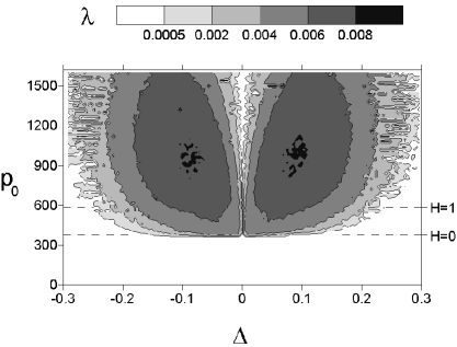
Figure 1: Maximum Lyapunov exponent $\lambda$ vs atom-field detuning $\Delta$ (in units of the laser Rabi frequency $\Omega$) and initial atomic momentum $p_{0}$ (in units of the photon momentum $\hbar k_{f}$): $\omega_{r}=10^{-5}$, $u_{0}=z_{0}=0.7071$, $v_{0}=0$.

In white regions the values of $\lambda$ are almost zero, and the atomic motion is regular in the corresponding ranges of $\Delta$ and $p_{0}$. In shadowed regions positive values of $\lambda$ imply unstable motion.

In all numerical simulations we shall use the normalized value of the recoil frequency equal to $\omega_{r}=10^{-5}$. The initial atomic position is taken to be $x_{0}=0$. The detuning $\Delta$ will be varied in a wide range, and the Bloch variables are restricted by the length of the Bloch vector (7). It should be noted that we use in this paper the normalization to the laser Rabi frequency $\Omega$, not to the vacuum (or single-photon) Rabi frequency as it has been done in our previous papers PK01 ; PS01 ; Pr02 ; JETP . So the ranges of the normalized control parameters, taken in this paper, differ from those in the cited papers. Figure 1 demonstrates that the center-of-mass motion becomes unstable if the dimensionless momentum exceeds the value $p_{0}\approx 300$ that corresponds (with our normalization) to the atomic velocity $v_{a}\approx 1$ m/s of a cesium atom in the field with the wavelength close to the transition wavelength $\lambda_{a}\simeq 852$ nm.

III Regimes of motion

III.1 Regular atomic motion at exact atom-field resonance

The case of exact resonance, $\Delta=0$, was considered in detail in Ref. PS01 ; JRLR . Now we briefly repeat the simple results for the sake of self-consistency. At zero detuning, the variable $u$ becomes a constant, $u=u_{0}$, and the fast ($u$, $v$, $z$) and slow ($x$, $p$) variables are separated allowing one to integrate exactly the reduced equations of motion. The total energy is equal to

$$H_{0}=\frac{\omega_{r}}{2}p^{2}-u\cos x,$$ (9)

where $u=u_{0}$. The center-of-mass atomic motion in this spatially periodic potential of the standing wave is described by the simple nonlinear equation for a free physical pendulum

$$\ddot{x}+\omega_{r}u_{0}\sin x=0,$$ (10)

and does not depend on evolution of the internal degrees of freedom.

The translational motion is trivial when $u_{0}$ is zero. The atom moves in one direction with a constant velocity, and the Rabi oscillations are modulated by the standing wave. Equations (9) and (10) describe the atomic motion in the simple cosine potential $u_{0}\cos x$ with three types of trajectories which are possible in dependence on the value of the energy $H$: oscillator-like motion in a potential well if $H_{0}<u_{0}$ (atoms are trapped by the standing-wave field Letokhov ), motion along the separatrix if $H_{0}=u_{0}$, and ballistic-like motion if $H_{0}>u_{0}$. Exact solutions of Eq. (10) are easily found in terms of elliptic functions (see PS01 ; JRLR ).

As to internal atomic evolution, it depends on the translational degree of freedom since the strength of the atom-field coupling depends on the position of atom in a periodic standing wave. At $\Delta=0$, it is easy to find the exact solutions of Eqs. (5)

$$v(\tau)=\pm\sqrt{1-u^{2}}\ \cos\left(2\int\limits_{0}^{\tau}\cos xd\tau^{\prime}+\chi_{0}\right),$$ (11)

$$z(\tau)=\mp\sqrt{1-u^{2}}\ \sin\left(2\int\limits_{0}^{\tau}\cos xd\tau^{\prime}+\chi_{0}\right),$$

where $u=u_{0}$, and $\cos[x(\tau)]$ is a given function of the translational variables only which can be found with the help of the exact solution for $x$ PS01 ; JRLR . The sign of $v$ is equal to that for the initial value $z_{0}$ and

$$\chi_{0}\equiv\mp\arcsin\frac{z_{0}}{\sqrt{1-u_{0}^{2}}}$$ (12)

is an integration constant. The internal energy of the atom, $z$, and its quadrature dipole-moment component $v$ could be considered as frequency-modulated signals with the instant frequency $2\cos[x(\tau)]$ and the modulation frequency $\omega_{r}p(\tau)$, but it is correct only if the maximum value of the first frequency is much greater than the value of the second one, i. e., for $|\omega_{r}p_{0}|\ll 2$.

III.2 Chaotic atomic transport off the resonance

In Fig. 1 we show the $\lambda$-map in the space of the initial momentum $p_{0}$ and detuning $\Delta$ values. The maximum Lyapunov exponent $\lambda$ depends both on the parameters $\omega_{r}$ and $\Delta$, and on initial conditions of the system (5). It is naturally to expect that off the resonance atoms with comparatively small values of the initial momentum $p_{0}$ will be at once trapped in the first well of the optical potential, whereas those with large values of $p_{0}$ will fly through. The question is what will happen with atoms, if their initial kinetic energy will be close to the maximum of the optical potential. Numerical experiments demonstrate that such atoms will wander in the optical lattice with alternating trappings in the wells of the optical potential and flights over its hills. The direction of the center-of-mass motion of wandering atoms may change in a chaotic way (in the sense of exponential sensitivity to small variations in initial conditions). A typical chaotic atomic trajectory is shown in Fig. 2.

Figure 2: Typical atomic trajectory in the regime of chaotic transport: $x_{0}=0$, $p_{0}=300$, $z_{0}=-1$, $u_{0}=v_{0}=0$, $\omega_{r}=10^{-5}$, $\Delta=-0.05$. Atomic position is shown in units of $k_{f}^{-1}$, time $\tau$ in units of $\Omega^{-1}$.

It follows from (5) that the translational motion of the atom at $\Delta\neq 0$ is described by the equation of a nonlinear physical pendulum with the frequency modulation

$$\ddot{x}+\omega_{r}u(\tau)\sin x=0,$$ (13)

where $u$ is a function of all the other dynamical variables.

IV Stochastic map for chaotic atomic transport

Chaotic atomic transport occurs even if the normalized detuning is very small, $|\Delta|\ll 1$ (Fig. 1). Under this condition, we will derive in this section approximate equations for the center-of-mass motion. The atomic energy at $|\Delta|\ll 1$ is given with a good accuracy by the simple resonant expression (9). Returning to the basic set of the equations of motion (5), we may neglect the first term in the fourth equation since it is very small as compared with the second one there. However, we cannot now exclude the third equation from the consideration. Using the solution (11) for $v$, we can transform this equation as

$$\dot{u}=\pm\Delta\sqrt{1-u^{2}}\ \cos\chi,$$ (14)

where

$$\chi\equiv 2\int\limits_{0}^{\tau}\cos xd\tau^{\prime}+\chi_{0}.$$ (15)

Far from the nodes of the standing wave, Eq. (14) can be approximately integrated under the additional condition, $|\omega_{r}p|\ll 1$, which is valid for the ranges of the parameters and the initial atomic momentum where chaotic transport occurs. Assuming $\cos x$ to be a slowly-varying function in comparison with the function $\cos\chi$, we obtain far from the nodes the approximate solution for the $u$-component of the atomic dipole moment

$$u\approx\sin\left(\pm\frac{\Delta}{2\cos x}\sin\chi+C\right),$$ (16)

where $C$ is an integration constant. Therefore, the amplitude of oscillations of the quantity $u$ for comparatively slow atoms ($|\omega_{r}p|\ll 1$) is small and of the order of $|\Delta|$ far from the nodes.

It follows from the third and forth equations in the set (5) that $u$ satisfies to the equation of motion for a driven harmonic oscillator with the natural frequency $|\Delta|$ and the driving force $2z\cos x$ whose frequency is space and time dependent. At $|\Delta|=0$, the synchronized component of the atomic dipole moment $u=$ is a constant whereas the other Bloch variables $z$ and $v$ oscillate in accordance with the solution (11). At $|\Delta|\neq 0$ and far from the nodes, the variable $u$ performs shallow oscillations for the natural frequency $|\Delta|$ is small as compared with the Rabi frequency. However, the behavior of $u$ is expected to be very special when an atom approaches to any node of the standing wave since near the node the oscillations of the atomic population inversion $z$ slow down and the corresponding driving frequency becomes close to the resonance with the natural frequency. As a result, sudden “jumps” of the variable $u$ are expected to occur near the nodes. This conjecture is supported by the numerical simulation. In Fig. 3 we show a typical behavior of the variable $u$ for a comparatively slow and slightly detuned atom.

Figure 3: Typical evolution of the atomic dipole-moment component $u$ for a comparatively slow and slightly detuned atom: $x_{0}=0$, $p_{0}=550$, $v_{0}=0$, $u_{0}=z_{0}=0.7071$, $\omega_{r}=10^{-5}$, $\Delta=-0.01$.

The plot clearly demonstrates sudden “jumps” of $u$ near the nodes of the standing wave and small oscillations between the nodes.

Approximating the variable $u$ between the nodes by constant values, we can construct a discrete mapping $u_{m}=f(u_{m-1})$, where $u_{m}$ is a value of $u$ just after the $m$-th node crossing (including multiple crossings of the same node). In order to estimate the values of $u$ just after the crossing, one needs to integrate Eq. (14) near a node. Since $u$ changes largely in a small region near nodes (so small that the atomic momentum has no time to change its value significantly) we may use the Raman-Nath approximation of the constant velocity. In this approximation, we have

$$\chi\simeq\frac{2}{\omega_{r}p_{\rm{node}}}\sin x+\chi_{0}.$$ (17)

Substituting this expression into Eq. (14), we can integrate it in the interval $0\leqslant x\leqslant\pi$ (which comprises only one node) and obtain the value of $u$ just after crossing the first node

$$u_{1}\approx\sin\left(\arcsin u_{0}\pm\frac{\Delta}{\omega_{r}p_{\rm{node}}}\int\limits_{0}^{\pi}\cos\chi dx\right)=$$ (18)

$$\ =\sin\left(\arcsin u_{0}\pm\frac{\Delta\pi}{\omega_{r}p_{\rm{node}}\sqrt{1-u_{0}^{2}}}\right.\times$$

$$\ \times\left[v_{0}J_{0}\left(\frac{2}{\omega_{r}p_{\rm{node}}}\right)+\left.z_{0}E_{0}\left(\frac{2}{\omega_{r}p_{\rm{node}}}\right)\right]\right),$$

where

$$p_{\rm{node}}\equiv\sqrt{\frac{2H}{\omega_{r}}}$$ (19)

is the value of the atomic momentum at the instant when the atom crosses a node (which is the same with a given value of the energy $H$ for all the nodes), $J_{0}$ and $E_{0}$ are zero-order Bessel and Weber functions, respectively. In the limit of the large argument $2/(\omega_{r}p_{\rm{node}})$, both the functions have a harmonic asymptotics Emde , and the expression (18) reduces to the form

$$u_{1}\approx\sin\left(\pm\frac{\Delta}{\sqrt{1-u_{0}^{2}}}\right. \left[\sqrt{\frac{\pi}{\omega_{r}p_{\rm{node}}}}\right.\times$$ (20)

$$\times\left(v_{0}\cos\left(\frac{2}{\omega_{r}p_{\rm{node}}}-\frac{\pi}{4}\right)\right.- \left.z_{0}\sin\left(\frac{2}{\omega_{r}p_{\rm{node}}}-\frac{\pi}{4}\right)\right)-$$

$$-\left.\left.z_{0}\right]+\arcsin u_{0}\right).$$

It is the deterministic solution obtained with the approximations mentioned above. It should be stressed that the solution contains trigonometric functions with large values of the arguments which are inversely proportional to the atomic momentum. In the Raman-Nath approximation, we take $p\simeq p_{\rm{node}}$. In fact, even small deviations from this mean value may result in large changes in the magnitude of the trigonometric functions. Therefore, they can be treated as, practically random variables in the range $[-1,1]$. Beyond the Raman-Nath approximation, the value of the atomic momentum $p$ depends on the value of $u_{m}$ which changes every time when the atom crosses a node. So, we can replace arguments of the trigonometric functions by random variables. Finally, we introduce the stochastic map

$$u_{m}\equiv\sin\left(\Delta\sqrt{\frac{\pi}{\omega_{r}p_{\rm{node}}}}\sin\phi_{m}+\arcsin u_{m-1}\right)=$$ (21)

$$=\sin\left(\Delta\sqrt{\frac{\pi}{\omega_{r}p_{\rm{node}}}}\sum\limits_{j=1}^{m}\sin\phi_{j}+\arcsin u_{0}\right),$$

where $\phi_{m}$ are random phases to be chosen in the range $[0,2\pi]$. When deriving this map, we neglected the term $z_{0}$ in Eq. (20) which is small as compared with the factor $\sqrt{\pi/\omega_{r}p_{\rm{node}}}$.

With given values of $\Delta$, $\omega_{r}$, and $p_{\rm{node}}$, the map (21) has been shown numerically to give a satisfactory probabilistic distribution of magnitudes of changes in the variable $u$ just after crossing the nodes. The stochastic map (21) is valid under the assumptions of small detunings ($|\Delta|\ll 1$) and comparatively slow atoms ($|\omega_{r}p|\ll 1$). Furthermore, it is valid only for those ranges of the control parameters and initial conditions where the motion of the basic system (5) is unstable. For example, in those ranges where all the Lyapunov exponents are zero, $u$ becomes a quasi-periodic function and cannot be approximated by the map.

The stochastic map (21) allows to reduce the basic set of equations of motion (5) to the following effective equations of motion:

$$\dot{x} = \omega_{r}p,$$ (22)

$$\dot{p} = -u_{m}\sin x,$$

$$\dot{m} = \omega_{r}p_{\rm{node}}\ |\delta(\cos x)|,$$

where $u_{m}$ is found from Eq. (21). The third equation in the set (22) gives a correspondence between the continuous evolution of the atomic motion and a discrete crossing number $m$. The integration of the delta function $\delta(\cos x)$ over time at points with $\cos x=0$ gives $\pm 1/(\omega_{r}p_{\rm{node}})$ in dependence on the direction of motion and whether the serial number of the node is even or odd. Since we calculate absolute values of the delta function, it is easy to show that $m$ is a constant if $\cos x\neq 0$ and increases by one if $\cos x=0$.

V Statistical properties of chaotic transport

V.1 Model for chaotic atomic transport

With given values of the control parameters and the energy $H$, the center-of-mass motion is determined by the values of $u_{m}$ (see Eq. (13)). One can obtain from the expression for the energy (9) the conditions under which atoms continue to move in the same direction after crossing a node or change the direction of motion not reaching the nearest antinode. Moreover, as in the resonance case, there exist atomic trajectories along which atoms move to antinodes with the velocity going asymptotically to zero. It is a kind of separatrix-like motion with an infinite time of reaching the stationary points.

The conditions for different regimes of motion depend on whether the crossing number $m$ is even or odd. Motion in the same direction occurs at $(-1)^{m+1}u_{m}<H$, separatrix-like motion — at $(-1)^{m+1}u_{m}=H$, and turns — at $(-1)^{m+1}u_{m}>H$. It is so because even values of $m$ correspond to $\cos x>0$, whereas odd values — to $\cos x<0$. The quantity $u$ during the motion changes its values in a random-like manner (see Fig. 3) taking the values which provide the atom either to prolong the motion in the same direction or to turn. Therefore, atoms may move chaotically in the optical lattice. The chaotic transport occurs if the atomic energy is in the range $0<H<1$. At $H<0$, atoms cannot reach even the nearest node and oscillate in the first potential well in a regular manner (see Fig. 1). At $H>1$, the values of $u$ are always satisfy to the flight condition. Since the atomic energy is positive in the regime of chaotic transport, the corresponding conditions can be summarized as follows: at $|u|<H$, atom always moves in the same direction, whereas at $|u|>H$, atom either moves in the same direction, or turns depending on the sign of $\cos x$ in a given interval of motion. In particular, if the modulus of $u$ is larger for a long time then the energy value, then the atom oscillates in a potential well crossing two times each of two neighbor nodes in the cycle.

The conditions stated above allow to find a direct correspondence between chaotic atomic transport in the optical lattice and stochastic dynamics of the Bloch variable $u$. It follows from Eq. (21) that the jump magnitude $u_{m}-u_{m-1}$ just after crossing the $m$-th node depends nonlinearly on the previous value $u_{m-1}$. For analyzing statistical properties of the chaotic atomic transport, it is more convenient to introduce the map for $\arcsin u_{m}$

$$\theta_{m}\equiv\arcsin u_{m}=$$ (23)

$$=\Delta\sqrt{\frac{\pi}{\omega_{r}p_{\rm{node}}}}\sin\phi_{m}+\arcsin u_{m-1},$$

where the jump magnitude does not depend on a current value of the variable. The map (23) visually looks as a random motion of the point along a circle of unit radius (Fig. 4). The vertical projection

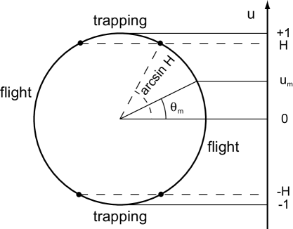
Figure 4: Graphic representation for the maps of $u_{m}$ and $\theta_{m}\equiv\arcsin u_{m}$. $H$ is a given value of the atomic energy. Atoms either oscillate in optical potential wells (trapping) or fly through the optical lattice (flight).

of this point is $u_{m}$. The value of the energy $H$ specifies four regions, two of which correspond to atomic oscillations in a well, and two other ones — to ballistic motion in the optical lattice.

We will call “a flight” such an event when atom passes, at least, two successive antinodes (and three nodes). The continuous flight length $L>2\pi$ is a distance between two successive turning points at which the atom changes the sign of its velocity, and the discrete flight length is a number of nodes $l$ the atom crossed. They are related in a simple way, $L\simeq\pi l$, for sufficiently long flight.

Center-of-mass oscillations in a well of the optical potential will be called “a trapping”. At extremely small values of the detuning (the exact criterion will be given below), the jump magnitudes are small and the trapping occurs, largely, in the $2\pi$-wide wells, i. e., in the space interval of the length $2\pi$. At intermediate values of the detuning, it occurs, largely, in the $\pi$-wide wells, i. e. in the space interval of the length $\pi$. Far from the resonance, $|\Delta|\gtrsim 1$, trapping occurs only in the $\pi$-wide wells. Just like to the case of flights, the number of nodes $l$, atom crossed being trapped in a well, is a discrete measure of trapping.

V.2 Statistics of chaotic atomic transport at large jump magnitudes of $u$

If the jump magnitudes of the variable $u$ are sufficiently large

$$|\Delta|\sqrt{\frac{\pi}{\omega_{r}p_{\rm{node}}}}\gtrsim\frac{\pi}{2},$$ (24)

then the internal atomic variable $\theta_{m}\equiv\arcsin u_{m}$ just after crossing the $m$-th node may take with the same probability practically any value from the range $[-\pi/2,\pi/2]$ (see Fig. 4). With given values of the recoil frequency $\omega_{r}=10^{-5}$ and the energy in the range $0<H<1$ corresponding to chaotically moving atoms, large jumps take place at medium detunings $|\Delta|\sim 0.1$. The probability $P_{-}$ for an atom to turn just after crossing a node is equal to the probability to get to one of the trapping regions in Fig. 4 (which one depends on whether the crossing number $m$ is even or odd) and is given by

$$P_{-}=\frac{\arccos H}{\pi}<\frac{1}{2},\quad P_{+}=1-P_{-},$$ (25)

where $P_{+}$ is the probability to prolong the motion in the same direction after crossing the node. It is easily to get from Eq. (25) the probability for an atom to cross $l$ successive nodes before turning

$$P_{\rm fl}(l)=P_{+}^{\ l}P_{-}=$$ (26)

$$=\left(\frac{\arccos H}{\pi}\right)\exp\left[l\ \ln\left(1-\frac{\arccos H}{\pi}\right)\right].$$

It is a flight probability density function (PDF) in terms of the discrete flight lengths. The exponential decay means that the atomic transport is normal for sufficiently large values of the jump magnitudes of the variable $u$.

The statistics of the center-of-mass oscillations in the potential wells can be obtained analogously. With large values of the jump magnitudes (24), trapping occurs, largely, in the $\pi$-wide wells. The probability for a trapped atom to cross the corresponding well node $l$ times before escaping from the well is

$$P_{\rm tr}(l)=P_{-}^{\ l}P_{+}=$$ (27)

$$=\left(1-\frac{\arccos H}{\pi}\right)\exp\left[l\ \ln\left(\frac{\arccos H}{\pi}\right)\right].$$

V.3 Statistics of chaotic atomic transport at small jump magnitudes of $u$

In this subsection we consider the case of small values of the jump magnitudes of the variable $u$

$$|\Delta|\sqrt{\frac{\pi}{\omega_{r}p_{\rm{node}}}}\ll\frac{\pi}{2}.$$ (28)

Now, it may take a long time for an atom to exit from one of the trapping or flight regions in Fig. 4. So, we need to calculate the time of exit of the random variable $\theta_{m}\equiv\arcsin u_{m}$ from one of these regions. The result will depend on what is the length of the corresponding circular arc in Fig. 4 as compared with the jump lengths.

Firstly, let us consider the case if the jump lengths are small as compared with the lengths both of the flight and trapping arcs, i. e., if

$$|\Delta|\sqrt{\frac{\pi}{\omega_{r}p_{\rm{node}}}}\ll{\rm{min}}\{\arcsin H,\arccos H\}.$$ (29)

Motion of $\theta_{m}$ along the circle can be now treated as a one-dimensional diffusion process for a fictitious particle described by the equation

$$\frac{\partial{\cal P}(\theta,m)}{\partial m}=D\frac{\partial^{2}{\cal P}(\theta,m)}{\partial\theta^{2}},$$ (30)

where ${\cal P}$ is a probability density to find the particle at the angular position $\theta$ just after crossing the $m$-th node and $D$ is the corresponding diffusion coefficient of the particle

$$D\equiv\frac{{\lang(\theta_{m}-\theta_{m-1})^{2}\rang}-{\lang\theta_{m}-\theta_{m-1}\rang}^{2}}{2}=\frac{\Delta^{2}\pi}{4\omega_{r}p_{\rm{node}}},$$ (31)

which was calculated for the particle jumping randomly with the mean magnitude ${\lang\theta_{m}-\theta_{m-1}\rang}$ (equal to zero in our case of symmetric jump distribution) and the variance ${\lang(\theta_{m}-\theta_{m-1})^{2}\rang}$. Thus, we reduced the task to the first passage time probability problem for a continuous Markov process. Using the results of this theory for a Wiener diffusion process Barucha described by Eq. (31), we calculate the probability density for a particle to exit from the interval $\theta_{c}\pm\theta_{\rm{max}}$ after crossing $l$ nodes

$$P(l)=\frac{2\pi D}{\theta^{2}_{\rm{max}}}\sum\limits_{j=0}^{\infty}(-1)^{j}(j+1/2)\times$$ (32)

$$\times\cos\left[(j+1/2)\frac{\pi(\theta_{0}-\theta_{c})}{\theta_{\rm{max}}}\right]\exp\frac{-(j+1/2)^{2}\pi^{2}Dl}{\theta^{2}_{\rm{max}}},$$

where $\theta_{0}$ is an initial angular position of the particle in the region under consideration and $\theta_{c}$ is the center of the region (with four possible values $0$, $\pi/2$, $\pi$, $3\pi/2$).

Since in a case of small jumps a particle gets to the region near its limit point, it is possible to replace $\theta_{0}$ by the quantity $\theta_{0}=\theta_{c}-\theta_{\rm{max}}+\epsilon$ with a small positive value of $\epsilon$. Expanding the cosine in (32) in the vicinity of the nodes and taking into account only the terms of the first order of smallness, we get the flight and trapping PDFs

$$P_{\rm fl}(l)\simeq\frac{Q}{\arcsin^{3}H} \sum\limits_{j=0}^{\infty}(j+1/2)^{2}\times$$ (33)

$$\times\exp\frac{-(j+1/2)^{2}\pi^{2}Dl}{\arcsin^{2}H},$$

$$P_{\rm tr}(l)\simeq\frac{Q}{\arccos^{3}H} \sum\limits_{j=0}^{\infty}(j+1/2)^{2}\times$$

$$\times\exp\frac{-(j+1/2)^{2}\pi^{2}Dl}{\arccos^{2}H},$$

where $Q$ is a normalization constant that is the same in both the cases. When deriving the first and second expressions (33), we replaced $\theta_{\rm{max}}$ by $\arcsin H$ and $\arccos H$, respectively. It is easily to realize that when $j$ exceeds the value $\theta_{\rm{max}}/(\pi\sqrt{Dl})$, the corresponding terms of the series (33) decrease rapidly.

The PDFs (33) can be written in a much more simple form for two conditions imposed on the number of jumps (node crossings) $l$ a particle needs to quit the interval $\theta_{c}\pm\theta_{\rm{max}}$. If $l\gtrsim\theta^{2}_{\rm{max}}/D$, then all the terms in the sums (33) are small as compared with the first one. Both the flight and trapping statistics are exponential in this case.

To the contrary, if $l\ll\theta^{2}_{\rm{max}}/D$, then one should take into account a large number of terms in the sums (33), and each sum can be replaced approximately by the integral. In this case the result does not depend on the length of the region $2\theta_{\rm{max}}$ and we get the power law decay

$$P(l)\simeq\frac{Q}{\theta^{3}_{\rm{max}}}\int\limits_{0}^{\infty}(j+1/2)^{2}\exp\frac{-(j+1/2)^{2}\pi^{2}Dl}{\theta^{2}_{\rm{max}}}dj\simeq$$ (34)

$$\simeq\frac{Q\pi^{-2.5}D^{-1.5}}{4}l^{-1.5},\quad l\ll\frac{\theta^{2}_{\rm{max}}}{D}$$

both for the flight and trapping PDFs. The power-law statistics (34) implies anomalous atomic transport. Dividing the length $2\theta_{\rm{max}}$ by the jump magnitude (28), we obtain the quantity

$$l_{\rm{cr}}\equiv\theta_{\rm{max}}/\sqrt{D}$$ (35)

that is a minimum number of jumps (node crossings) a particle needs to pass the region through. With the number of jumps $l<l_{\rm{cr}}$, a particle, randomly moving on the circle, may get out of the interval $\theta_{c}\pm\theta_{\rm{max}}$ only through the same border where it got in. The statistics of exit times is known to be a power-law one with the transport exponent equal to $-1.5$. The length of the interval does not matter in this case. If $l\gtrsim l_{\rm{cr}}$, then particles may exit through both the borders, and the corresponding statistics cannot be approximated by a single transport exponent. If $l\gtrsim l^{2}_{\rm{cr}}\equiv\theta^{2}_{\rm{max}}/D$, then we expect an exponential decay.

The size of the trapping and flight regions depends on the value of the atomic energy $H$ (see Fig. 4). At $H>\sqrt{2}/2$ ($\arcsin H>\pi/4$), the flight PDF has a longer decay than the trapping PDF. On the contrary, at $H<\sqrt{2}/2$, the $P_{\rm tr}$’s decay is longer than the $P_{\rm fl}$’s one. If the jump magnitude (28) is of the order of the size of the flight or trapping regions

$$|\Delta|\sqrt{\frac{\pi}{\omega_{r}p_{\rm{node}}}}\sim\arcsin H\ll\frac{\pi}{2},$$ (36)

$${\rm{or}}$$

$$|\Delta|\sqrt{\frac{\pi}{\omega_{r}p_{\rm{node}}}}\sim\arccos H\ll\frac{\pi}{2},$$

then a particle may pass through the region making a small number of jumps $l$. So, the approximation of the diffusion process (29) fails, and the corresponding PDF is exponential.

Figure 5: The flight $P_{\rm fl}$ and trapping $P_{\rm tr}$ PDFs for a chaotically moving atom with comparatively small values of the jump magnitudes of the variable $u$. The detuning $\Delta=-0.001$ is small, and the energy value $H=0.724$ ($p_{0}=535$) provides approximately equal sizes of the flight and trapping regions in Fig. 4. White and black circles represent results of integration of the basic (5) and reduced (22) equations of motion, respectively, and the solid lines represent the analytical PDFs (33). $x_{0}=0$, $z_{0}=-1$, $u_{0}=v_{0}=0$, $\omega_{r}=10^{-5}$.

In order to check the analytical results obtained in this section, we compare them with numerical simulation of the reduced (22) and basic (5) equations of motion. The reduced equations (22) describe the center-of-mass motion modulated by a jump-like behavior of the internal variable $u$ which satisfies to the stochastic map (21). To explore different regimes of the chaotic atomic transport we integrate Eqs. (22) and (5) numerically with two values of the detuning $\Delta=-0.001$ and $\Delta=-0.01$ (the cases of small and medium jump magnitudes of the variable $u$, respectively) and different values of the atomic energy and momentum and compute the PDFs of the flight and trapping events. They are normalized histograms for a number of standing-wave nodes $l$ which the atom crossed in a run. Each PDF is computed with a single but very long (up to $\tau\sim 10^{8}$ for the basic equations of motion) atomic trajectory.

Figure 6: The same as in Fig. 5 but with the energy $H=0.101$ ($p_{0}=402$) providing a narrow flight region as compared with the trapping one.

In Fig. 5 we compare the results (in a log-log scale) in the case of small jump magnitudes of the variable $u$ ($\Delta=-0.001$) and approximately equal sizes of the flight and trapping regions ($H=0.724\sim\sqrt{2}/2$). White and black circles represent the results of numerical integration of the basic (5) and reduced (22) equations of motion, respectively, and the solid line represents the analytical predictions (33). The agreement between the PDFs computed with Eqs. (5), (22), and (33) is rather good. All the flight and trapping PDFs exhibit in their dependence on the crossing number $l$ three kinds of decay which are fairly approximated by the formulas (33). The critical value of the crossing number $l$ is estimated to be $l_{\rm{cr}}\simeq 55$ with chosen values of the parameters and initial conditions. In the range $l\lesssim 55$ the PDFs are expected to demonstrate the power law decay with the slope $-1.5$ given by the formula (34). In the range $55\lesssim l\lesssim l^{2}_{\rm{cr}}\simeq 3000$, there should exist a number of different transport exponents. The initial part of this range is fitted by the same power-law function. However, the other part of the range cannot be fitted by a simple function. In the range $l\gtrsim l^{2}_{\rm{cr}}\simeq 3000$, the decay is expected to be purely exponential in accordance with the the first expression in Eqs. (33).

In Fig. 6 we show the PDFs computed at the same detuning $\Delta=-0.001$ as in Fig. 5 but with the value of the atomic energy $H=0.101$ for which the flight region in Fig. 4 is narrower than the trapping one. The jump magnitude is now of the order of the length of the flight region (see (36)) and the flight PDFs are expected to be exponential ($l_{cr}\simeq 9$). The critical value of the crossing number $l$ for trapping is $l_{\rm{cr}}\simeq 58$ with given values of the energy and the detuning. Therefore, in the range $l\lesssim 58$ the trapping PDFs are expected to vary as the power law decay with the slope $-1.5$ given by the formula (34). In the range $l\gtrsim l^{2}_{\rm{cr}}\simeq 3400$, the decay is expected to be purely exponential in accordance with the the second expression in Eqs. (33). The trapping PDFs in the range $58\lesssim l\lesssim l^{2}_{\rm{cr}}\simeq 3400$ are neither power law nor exponential demonstrating a complicated behavior. This speculation is confirmed by the numerical computation shown in Fig. 6.

Figure 7: The flight $P_{\rm fl}$ and trapping $P_{\rm tr}$ PDFs for a chaotically moving atom with comparatively large values of the jump magnitudes of the variable $u$. The detuning $\Delta=-0.01$ is medium, and the energy value $H=0.8055$ ($p_{0}=550$) provides a domination of the flight events over the trapping ones. White and black circles represent results of integration of the basic (5) and reduced (22) equations of motion, respectively, and the solid lines represent the analytical PDFs (33). $x_{0}=0$, $z_{0}=-1$, $u_{0}=v_{0}=0$, $\omega_{r}=10^{-5}$.

In order to demonstrate what happens with larger values of the jump magnitudes, we take the detuning to be $\Delta=-0.01$ increasing the jump magnitude in ten times as compared with the preceding cases. With the taken value of the energy $H=0.8055$ we provide a slight domination of flights over trappings. The jump magnitude is now so large that particles may pass both through the flight and trapping regions making a small number of jumps. It is expected that all the PDFs, both the flight and trapping ones, should be practically exponential in the whole range of the crossing number $l$. It is really the case (see Fig. 7).

VI Dynamical fractals

Various fractal-like structures may arise in chaotic Hamiltonian systems Ott ; 13 ; 14 . In our previous papers JETP ; JRLR we have found numerically fractal properties of chaotic atomic transport in cavities and optical lattices. In this section we apply the analytical results of the theory of chaotic transport, developed in the preceding sections, to find the conditions under which the dynamical fractals may arise.

We place atoms one by one at the point $x_{0}=0$ with a fixed positive value of the momentum $p_{0}$ and compute the time $T$ when they cross one of the nodes at $x=-\pi/2$ or $x=3\pi/2$. In these numerical experiments we change the value of the atom-field detuning $\Delta$ only. All the initial conditions $p_{0}=200$, $z_{0}=-1$, $u_{0}=v_{0}=0$ and the recoil frequency $\omega_{r}=10^{-5}$ are fixed.

Figure 8: Fractal-like dependence of the time of exit of atoms $T$ from a small region in the optical lattice on the detuning $\Delta$: $p_{0}=200$, $z_{0}=-1$, $u_{0}=v_{0}=0$. Magnifications of the detuning intervals are shown.

The exit time function $T(\Delta)$ in Fig. 8 demonstrates an intermittency of smooth curves and complicated structures that cannot be resolved in principle, no matter how large the magnification factor. The second and third panels in Fig. 8 demonstrate successive magnifications of the detuning intervals shown in the upper panel. Further magnifications reveal a self-similar fractal-like structure that is typical for Hamiltonian systems with chaotic scattering Ott ; 14 . The exit time $T$, corresponding to both smooth and unresolved $\Delta$ intervals, increases with increasing the magnification factor. Theoretically, there exist atoms never crossing the border nodes at $x=-\pi/2$ or $x=3\pi/2$ in spite of the fact that they have no obvious energy restrictions to do that. Tiny interplay between chaotic external and internal atomic dynamics prevents those atoms from leaving the small space. The similar phenomenon in chaotic scattering is known as dynamical trapping. In Ref. JETP we have computed the Hausdorff dimension for the similar fractal and shown that it is not an integer. We note that the fractal-like structures similar to that shown in Fig. 8 arise in numerical experiments with longer distances between the border nodes but the corresponding computation time increases significantly with increasing this distance.

Various kinds of atomic trajectories can be characterized by the number of times $m$ atom crosses the central node at $x=\pi/2$ between the border nodes. There are also special separatrix-like trajectories along which atoms asymptotically reach the points with the maximum of the potential energy, having no more kinetic energy to overcome it. In difference from the separatrix motion in the resonant system ($\Delta=0$) with the initial atomic momentum $p_{\rm{cr}}$, a detuned atom can asymptotically reach one of the stationary points even if it was trapped for a while in a well. We specify the $mS$-trajectory as a trajectory of an atom crossing the central node $m$ times before starting the separatrix-like motion. Such an asymptotical motion takes an infinite time, so the atom will never reach the border nodes.

The smooth $\Delta$ intervals in the first-order structure (Fig. 8, upper panel) correspond to atoms which never change the direction of motion ($m=1$) and reach the border node at $x=3\pi/2$. The singular points in the first-order structure with $T=\infty$, which are located at the border between the smooth and unresolved $\Delta$ intervals, are generated by the $1S$-trajectories. Analogously, the smooth and unresolved $\Delta$ intervals in the second-order structure (second panel in Fig. 8) correspond to the 2-nd order ($m=2$) and the other trajectories, respectively, with singular points between them corresponding to the $2S$-trajectories, and so on.

There are two different mechanisms of generation of infinite exit times, namely, dynamical trapping with an infinite number of oscillations ($m=\infty$) inside the interval $[-\pi/2,3\pi/2]$ and the separatrix-like motion ($m\neq\infty$). The set of all the values of the detunings, generating the separatrix-like trajectories, was shown to be a countable fractal in Refs. JETP ; JRLR , whereas the set of the values generating dynamically trapped atoms with $m=\infty$ seems to be uncountable. The exit time $T$ depends in a complicated way not only on the values of the control parameters but on initial conditions as well. In Ref. JRLR we presented a two-dimensional image of this function in two coordinates of the initial atomic momentum $p_{0}$ and the atom-field detuning $\Delta$.

The fractal-like structure with smooth and unresolved components may appear if atoms have an alternative either to turn back or to prolong the motion in the same direction just after crossing the node at $x=\pi/2$. For the first-order structure in the upper panel in Fig. 8, it means that the internal variable $u$ of an atom, just after crossing the node for the first time ($\cos x<0$), satisfies either to the condition $u_{1}<H$ (atom moves in the same direction), or to the condition $u_{1}>H$ (atom turns back). If $u_{1}=H$, then the exit time $T$ is infinite. The jumps of the variable $u$ after crossing the node are deterministic but sensitively dependent on the values of the control parameters and initial conditions. We have used this fact when introducing the stochastic map in Sec. IV. Small variations in these values lead to oscillations of the quantity $\arcsin u_{1}$ around the initial value $\arcsin u_{0}$ with the amplitude $|\Delta|\sqrt{\pi/(\omega_{r}p_{\rm{node}})}$. If this amplitude is large enough, then the sign of the quantity $u_{1}-H$ alternates and we obtain alternating smooth (atoms reach the border $x=3\pi/2$ without changing their direction of motion) and unresolved (atoms turns a number of times before exit) components of the fractal-like structure. The singular points at the border of such components correspond to the atoms with infinite exit time.

If the values of the parameters admit large jump magnitudes of the variable $u$ (see condition (24)), then the dynamical fractal arises in the energy range $0<H<1$, i. e., at the same condition under which atoms move in the optical lattice in a chaotic way. In a case of small jump magnitudes, fractals may arise if the initial value of an atom $u_{0}$ is close enough to the value of the energy $H$, i.e., the atom has a possibility to overcome the value $u=H$ in one jump. Therefore, the condition for appearing in the fractal $T(\Delta)$ the first-order structure with singularities is the following:

$$|\arcsin u_{0}-\arcsin H|<|\Delta|\sqrt{\frac{\pi}{\omega_{r}p_{\rm{node}}}}.$$ (37)

The formation of the second-order structure is explained analogously. If an atom made a turn after crossing the node for the first time, then it will cross the node for the second time. After that, the atom either will turn or cross the border node at $x=-\pi/2$. What will happen depend on the value of $u_{2}$. However, in difference from the case with $m=1$, the condition for appearing an infinite exit time with $m=2$ is $u_{2}=-H$. Furthermore, the previous value $u_{1}$ is not fixed (in difference from $u_{0}$) but depends on the value of the detuning $\Delta$. In any case we have $u_{1}>H$ since the second-order structure consists of the trajectories of those atoms which turned after the first node crossing. Near the singular borders of the second-order structure we have $u_{1}\simeq H$, whereas far from them $u_{1}$ may be much larger. In order for an atom would be able to turn after the second node crossing, the magnitude of its variable $u$ should change sufficiently to be in the range $u_{2}<-H$. The atoms, whose variables $u$ could not “jump” so far, leave the space $[-\pi/2,3\pi/2]$. The singularities are absent in the middle part of the second-order structure shown in the second panel in Fig. 8 because all the corresponding atoms left the space after the second node crossing. The variable $u_{2}$ oscillates with varying $\Delta$ generating oscillations of the exit time. In vicinity of the borders of the second-order structure the required jump magnitude $u_{2}-u_{1}$ is smaller and is equal approximately to $2H$. Some atoms could turn for the second time or follow separatrix-like trajectories which generate singularities of the exit-time function. So, the condition for appearing singularities in the second-order structure is the following:

$$2\arcsin H<|\Delta|\sqrt{\frac{\pi}{\omega_{r}p_{\rm{node}}}}.$$ (38)

With the values of the parameters taken in the simulation, we get the energy $H=0.2+\Delta/2$. It is easy to obtain from the inequality (38) the approximate value of the detuning $|\Delta|\approx 0.0107$ for which the second-order singularities may appear. In the lower panel in Fig. 8 one can see this effect. No additional conditions are required for appearing the structures of the third and the next orders.

It should be noted that the inequality (38) is opposite to the first part of the inequality (29) that determines the condition for appearing power law decays in the flight PDF. Therefore, dynamical fractal may appear in those ranges of the control parameters where the Lévy flights are impossible and vice versa. However, the trapping PDF may have a power law decay. It should be noted that the inequality (38) in difference from (37) is strongly related with the chosen concrete scheme for computing exit times. It is not required with other schemes, say, with three antinodes between the border nodes.

VII Conclusion and discussion

We have studied semiclassical transport of atoms in a one-dimensional optical lattice in the framework of the idealized model of the atom-field interaction. The center-of-mass motion is strongly affected by the evolution of the atomic Bloch variables — the synchronized and quadrature components of the atomic dipole moment $u$ and $v$ and the population inversion $z$. There are ranges of the atom-field detuning $\Delta$ and the initial momentum $p_{0}$ where the atomic transport has been shown to be chaotic with a complicated alternation of trappings in wells of the optical potential and flights over them. We developed a semiclassical theory of the chaotic atomic transport in optical lattices in terms of a random walk of the Bloch variable $u$ and confirmed the analytical results by direct numerical simulation of the basic and reduced equations of motion.

Based on a jump-like behavior of the internal variable $u$ for atoms crossing nodes of the standing laser wave, we constructed a stochastic map that determines the center-of-mass motion. We found the relations between the detuning $\Delta$, recoil frequency $\omega_{r}$, and the atomic energy $H$, under which atoms may move in the lattice in a chaotic way. To illustrate statistical properties of the chaotic transport, we proposed a simple model of random walking of the quantity $\arcsin u$ on a circle.

The statistical properties of chaotic atomic transport strongly depend on the relation between the jump magnitude of the variable $u$ and the atomic energy. Both the length of flight and the duration of trapping are measured by a number of nodes $l$ atom crossed during the flight and trapping events, respectively. The PDFs for the flight $P_{\rm fl}(l)$ and trapping $P_{\rm tr}(l)$ events were analytically derived to be exponential in a case of large jumps. In a case of small jumps, the kind of the statistics depends on additional conditions imposed on the atomic and lattice parameters, and the distributions $P_{\rm fl}(l)$ and $P_{\rm tr}(l)$ were analytically shown to be either practically exponential or functions with long power law parts with the slope $-1.5$ but exponential “tails”. The comparison of the PDFs computed with analytical formulas, the stochastic map, and the basic equations of motion has shown a good agreement in different ranges of the atomic and lattice parameters. We used the results obtained to find the analytical conditions, under which the fractal properties of the chaotic atomic transport were observed, and to explain the structure of the corresponding dynamical fractals.

Since the period and amplitude of the optical potential and the atom-field detuning can be modified in a controlled way, the transport exponents of the flight and trapping distributions are not fixed but can be varied continuously, allowing to explore different regimes of the atomic transport. Our analytical and numerical results with the idealized system have shown that deterministic atomic transport in an optical lattice cannot be just classified as normal and anomalous one. We have found that the flight and trapping PDFs may have long algebraically decaying parts and a short exponential “tail”. It means that in some ranges of the atomic and lattice parameters numerical experiments reveal anomalous transport with Lévy flights (see Figs. 5 and  6). The transport exponent equal to $-1.5$ means that the first, second, and the other statistical moments are infinite for a reasonably long time. The corresponding atomic trajectories computed for this time are self-similar and fractal. The total distance, that the atom travels for the time when the flight PDF decays algebraically, is dominated by a single flight. However, the asymptotical behavior is close to normal transport. In other ranges of the atomic and lattice parameters, the transport is practically normal both for short and long times (see Fig. 7).

In conclusion we should emphasize that the theory of chaotic atomic transport in an optical lattice presented in this paper does not take into account spontaneous emission which is inevitable in any real experiment. Speculation about small changes in the atomic momentum of the order of $\hbar k_{f}$ (caused by spontaneous emission) as compared with its initial values of the order of $300\div 500\hbar k_{f}$ used in our computations is not a convincing argument because the atomic momentum is equal to zero at turning points, and spontaneous emission may change the center-of-mass motion in vicinity of these points. Spontaneous emission can be incorporated in the equations of motion of the type of our basic equations (5) AP06 by the quantum Monte Carlo method Carmichael . In general, we expect a competition between the coherent but chaotic atomic dynamics and random processes of spontaneous emission. In particular, the stochastic map (21) constructed in this paper should be generalized to include jumps of the variable $u$ to the zero value at random time moments. What will happen with the flight and trapping PDFs is an open question. We plan to study the atomic transport in an optical lattice with spontaneous emission in the future.

VIII Acknowledgments

This work was supported by the Russian Foundation for Basic Research (project no. 06-02-16421), by the Program ”Mathematical methods in nonlinear dynamics”of the Prezidium of the Russian Academy of Sciences, and the program of the Prezidium of the Far-Eastern Division of the Russian Academy of Sciences.

References

- (1) F. Bardou, J.P. Bouchaaud, A. Aspect, C. Cohen-Tannoudji, Lévy Statistics and Laser Cooling, Cambridge University Press, Cambridge (2002).
- (2) F. Bardou, J.P. Bouchaaud, O. Emile, A. Aspect, C. Cohen-Tannoudji, Phys. Rev. Lett. 72, 203 (1994).
- (3) C. Jurczak, B. Desruelle, K. Sergstock, J.-Y. Courtois, C. I. Westbrook, and A. Aspect, Phys. Rev. Lett. 77, 1727 (1996).
- (4) H. Katori, S. Schlipf, H. Walther, Phys. Rev. Lett. 79, 2221 (1997).
- (5) B.G. Klappauf, W.H. Oskay, D.A. Steck, and M.G. Raizen, Phys. Rev. Lett. 81, 4044 (1998).
- (6) B. Saubameá, M. Leduc, and C. Cohen-Tannoudji, Phys. Rev. Lett. 83, 3796 (1999).
- (7) G. Grynberg and C. Robilliard, Phys. Rep. 355, 335 (2001).
- (8) S. Marksteiner, K. Ellinger, P. Zoller, Phys. Rev. A 53, 3409 (1996).
- (9) W. Greenwood, P. Pax, and P. Meystre, Phys. Rev. A 56, 2109 (1997).
- (10) S. Schaufler, W. P. Schleich, and V. P. Yakovlev, Phys. Rev. Lett. 83, 3162 (1999).
- (11) E. Lutz, Phys. Rev. Lett. 93, 190602 (2004).
- (12) J.-P. Bouchaud and A. Georges, Phys. Rep. 195, 127 (1990).
- (13) M.F. Shlesinger, G. M. Zaslavsky, and J. Klafter, Nature 363, 31 (1993).
- (14) S. V. Prants and L. E. Kon’kov, JETP Letters, 73, 180 (2001) [Pis’ma ZhETF 73, 200 (2001)].
- (15) S. V. Prants and V. Yu. Sirotkin, Phys. Rev. A, 64, art. 033412 (2001).
- (16) S. V. Prants, JETP Letters 75, 651 (2002) [Pis’ma ZhETF 75, 777 (2002)].
- (17) V. Yu. Argonov and S. V. Prants, JETP 96, 832 (2003) [Zh. Eksp. Teor. Fiz. 123, 946 (2003)].
- (18) S. V. Prants, M. Edelman, G. M. Zaslavsky, Phys. Rev. E 66, 046222 (2002).
- (19) V. Gubernov, Phys. Rev. A 66, 013408 (2002).
- (20) S. V. Prants, M. Yu. Uleysky, Phys. Lett. A 309, 357 (2003).
- (21) S. V. Prants, M. Yu. Uleysky, and V. Yu. Argonov, Phys. Rev. A 73, 023807 (2006).
- (22) V. Yu. Argonov and S. V. Prants, Acta Phys. Hung. B 26, N 1–3, (2006)
- (23) V. Yu. Argonov and S. V. Prants, Journal of Russian Laser Research 27, 360 (2006).
- (24) A. J. Lichtenberg, M. A. Lieberman, Regular and Stochastic Motion, Springer, New York (1983).
- (25) V. S. Letokhov, JETP Lett. 7, 348 (1968) [Pis’ma ZhETF 7, 348 (1968)].
- (26) E. Ott, Chaos in dynamical systems, Cambridge University Press, Cambridge (1993).
- (27) E. Janke, F. Emde, F. Lösch, Tafeln Höherer Funktionen, B. G. Teubner Verlagsgesellschaft, Stuttgart (1960).
- (28) A. T. Bharucha-Reid, Elements of the Theory of Markov Processes and Their Applications, Mc Graw-Hill Book Company inc., New York – Toronto – London (1960).
- (29) G. M. Zaslavsky, Hamiltonian Chaos and Fractional Dynamics, Oxford University Press, Oxford (2005).
- (30) P. Gaspard, Chaos, Scattering and Statistical Mechanics, Cambridge University Press, Cambridge (1998).
- (31) H. Carmichael, An Open Systems Approach to Quantum Optics, Springer-Verlag, Berlin (1993); K. Molmer, Y. Castin, and J. Dalibard, J. Opt. Soc. Am. B 10, 524 (1993).