Localization of coherent exciton transport in phase space

Abstract

We study numerically the dynamics of excitons on discrete rings in the presence of static disorder. Based on continuous-time quantum walks we compute the time evolution of the Wigner function (WF) both for pure diagonal (site) disorder, as well as for diagonal and off-diagonal (site and transfer) disorder. In both cases, large disorder leads to localization and destroys the characteristic phase space patterns of the WF found in the absence of disorder.

I Introduction

Ever since the emergence and development of quantum mechanics, there has been a major interest in the crossover from quantum mechanical transport to the corresponding classical transport. However, there are far-reaching differences in the usual mathematical description of the two different processes. In classical physics, the phase space is spanned by conjugate variables, such as position and momentum, whose time development leads to classical transport. Quantum mechanical processes, on the contrary, take place in Hilbert space. One approach to overcome these differences was already presented in the early days of quantum mechanics, more than 70 years ago, by Wigner Wigner (1932); Hillery et al. (1984). He introduced a function, now known as Wigner function (WF), which is a (quasi) probability in a quantum mechanical phase space spanned by position and momentum variables. The WF is a real valued function and in this respect compares well with the classical Boltzmann probability distribution in phase space. However, it is not always positive. WFs and related phase space functions, like the Husimi function, are widely used in Quantum Optics Schleich (2001); Mandel and Wolf (1995) but also for describing electronic transport, see e.g. Kluksdahl et al. (1989); Buot (1993); Bordone et al. (1999).

Apart from the quantum-classical crossover there are also extremely interesting purely quantum mechanical phenomena. For example, Anderson has shown that there is no quantum diffusion for some random lattices Anderson (1958, 1978); Abrahams et al. (1979), an effect nowadays called (strong) localization, where the quantum mechanical transport through the lattice is, in essence, prohibited by the potential energy surface. Anderson’s hopping model for electron transport has also turned out to be useful in describing excitons in disordered systems, e.g., Logan and Wolynes (1987); Abramavicius et al. (2004); Dominguez-Adame and Malyshev (2004); Helmes et al. (2005); Barford and Duffy (2006).

In fact, Anderson’s model is closely related to the so-called continuous-time quantum walks (CTQWs) with disorder. Recently, it has been shown that the motion on a graph, described by CTQWs, can be exponentially suppressed by the disorder Keating et al. (2006). Originally, (unperturbed) CTQWs were introduced in the context of quantum information as the quantum mechanical analog of continuous-time random walks (CTRWs) Farhi and Gutmann (1998). Here, the underlying, discrete connectivity of the structure on which the transport takes place determines the Hamiltonian. Since CTQWs also model exciton transport over various discrete structures Mülken et al. (2006), they are closely connected to other appraches to study (coherent) exciton transport phenomena on discrete graphs, for instance, in the contexts of polymer Kenkre and Reineker (1982), atomic Shore (1990) or solid-state Haken (1976) physics.

In this paper we consider the dynamics of excitons on discrete rings under static disorder, focussing on a quantum mechanical phase space approach. We compute the corresponding WFs numerically and study the effects of both pure diagonal (site) disorder, as well as of diagonal and off-diagonal (site and transfer) disorder on the (coherent) transport. The WFs are then compared to the unperturbed case, for which an analytical treatment is possible Mülken and Blumen (2006).

The paper is organized as follows. In Sec. II we briefly review how we model coherent exciton transport on graphs and define the appropriate Hamiltonian for rings with two types of disorder. After introducing the discrete WF in Sec. III, we lay down the procedure of our calculations in Sec. IV. The subsequent Secs. V to VII show the numerical results for coherent exciton transport on rings with disorder. We close with our conclusions.

II Coherent exciton dynamics

In the absence of disorder, the (coherent) dynamics of excitons on a graph of connected nodes is modelled by the CTQW. Here, the CTQW is obtained by identifying the Hamiltonian of the system with the (classical) transfer matrix, ${\bf H}=-{\bf T}$, see e.g. Farhi and Gutmann (1998) (we will set $\hbar\equiv 1$ in the following). The transfer matrix of the walk, ${\bf T}=(T_{l,j})$, can be related to the connectivity matrix ${\bf A}$ of the graph by ${\bf T}=-\gamma{\bf A}$, where for simplicity we assume the transmission rates $\gamma$ of all bonds to be equal. The matrix ${\bf A}$ has as non-diagonal elements $A_{l,j}$ the values $-1$ if nodes $l$ and $j$ of the graph are connected by a bond and $0$ otherwise. The diagonal elements $A_{j,j}$ of ${\bf A}$ equal the number of bonds $f_{j}$ which exit from node $j$.

Now, the states $|j\rangle$ associated with excitations localized at the nodes $j$ span the whole accessible Hilbert space to be considered here. In general, the time evolution of a state $|j\rangle$ starting at time $t_{0}=0$ is given by $|j;t\rangle=\exp(-i{\bf H}t)|j\rangle$. By denoting the eigenstates of ${\bf H}$ by $|\Phi_{\theta}\rangle$ and the eigenvalues by $E_{\theta}$ the transition probability reads $\pi_{l,j}(t)\equiv\left|\langle l|\exp(-i{\bf H}t)|j\rangle\right|^{2}=\left|\sum_{\theta}\exp(-iE_{\theta}t)\langle l|\Phi_{\theta}\rangle\langle\Phi_{\theta}|j\rangle\right|^{2}$.

II.1 Dynamics on rings without disorder

The unperturbed Hamiltonian for such a CTQW on a finite one-dimensional network of length $N$ with periodic boundary conditions (PBC) takes on the very simple form ${\bf H}^{0}|j\rangle=2|j\rangle-|j-1\rangle-|j+1\rangle$, where we have taken the transmission rate to be $\gamma\equiv 1$ and $j=0,1,\dots,N-1$. The eigenstates $|\Phi_{\theta}^{0}\rangle$ of the time independent Schrödinger equation ${\bf H}^{0}|\Phi_{\theta}^{0}\rangle=E_{\theta}^{0}|\Phi_{\theta}^{0}\rangle$ are Bloch states, which can be expressed as linear combinations of the states $|j\rangle$, see Refs. Mülken and Blumen (2005, 2006) for details.

II.2 Dynamics on rings with disorder

Now we introduce (static) disorder by adding to the unperturbed Hamiltonian ${\bf H}^{0}$ a disorder operator $\mathbf{\Delta}$, i.e., by setting ${\bf H}={\bf H}^{0}+{\mathbf{\Delta}}$. We let the disorder matrix $\mathbf{\Delta}=(\Delta_{l,j})$ have non-zero entries only at the positions for which $H_{l,j}\neq 0$. For different strengths of disorder, the elements $\Delta_{l,j}=\Delta_{j,l}$ are chosen randomly (drawn from a normal distribution with the mean value zero and the variance one), which we multiply by a factor of $\Delta$, which then can take values from the interval $[0,1/2]$. Note that under these assumptions for the (static) disorder the connectivity of the graph is essentially unchanged, i.e., there are no new connections created nor are existing connections destroyed. Therefore, the only non-zero matrix elements of ${\bf H}$ are those of the initial ${\bf A}$. The action of the new Hamiltonian ${\bf H}$ on a state $|j\rangle$ reads thus

$${\bf H}|j\rangle = \Big{(}{\bf H}^{0}+{\mathbf{\Delta}}\Big{)}|j\rangle=2|j\rangle-|j-1\rangle-|j+1\rangle$$ (1)

$$+ 2\Delta_{j,j}|j\rangle-\Delta_{j,j-1}|j-1\rangle-\Delta_{j,j+1}|j+1\rangle.$$

In the following we consider two cases of disorder:

(A) Diagonal disorder (DD), where $\Delta_{j,j}\neq 0$ and $\Delta_{l,j}=0$ for $l\neq j$. We assign a random number to each $\Delta_{j,j}$, a procedure which leads to $N$ random numbers.

(B) Diagonal and off-diagonal disorder (DOD), where we choose a random number for each $\Delta_{j,j}$ and for each $\Delta_{j,j-1}$. Thus, $2N$ random numbers are needed.

Introducing disorder into the system in this way has consequences for the relation between the CTQWs and the CTRWs. In CTRWs the transition rates, given by the entries of the the transfer matrix ${\bf T}$, are correlated, i.e., for each site the sum of the non-diagonal rates for transmission from it and the diagonal rate of leaving it are the same. In the cases considered here, a direct identification of the Hamiltonian ${\bf H}$ with a classical transfer matrix ${\bf T}$ is, in general, not possible anymore. However, the DOD and DD Hamiltonians are widely used in quantum mechanical nearest-neighbor hopping models, to which also the CTQWs belong. Furthermore, we still consider transport processes on graphs which have the connectivity matrix ${\bf A}$, but the direct connection between ${\bf H}$ and ${\bf T}$ is lost. Of course, one can maintain this connection by imposing constraints on the $\Delta$, e.g., by requiring that $2\Delta_{j,j}=\Delta_{j,j-1}+\Delta_{j,j+1}$ for all $j$.

III Wigner functions

The WF is a quasi-probability (in the sense that it can become negative) in the quantum mechanical phase space. For a phase space spanned by the continuous variables $X$ and $K$, the WF reads Wigner (1932); Hillery et al. (1984); Schleich (2001)

$$W(X,K;t)=\frac{1}{\pi}\int\ dY\ e^{iKY}\ \langle X-Y/2|\hat{\rho}(t)|X+Y/2\rangle,$$ (2)

where $\hat{\rho}(t)$ is the density operator. In the following we only consider pure states, i.e., $\hat{\rho}(t)=|j;t\rangle\langle j;t|$. Note that the WF is normalized to one when integrated over the whole phase space.

For a discrete system having $N$ sites on a ring, where we choose to enumerate the sites as $0,1,\dots,N-1$, $\langle x|j;t\rangle$ is only defined for integer values of $x=0,1,\dots,N-1$, and the form of Eq.(2) has to be changed from an integral to a sum. Now the WF resembles a discrete Fourier transform, which requires $N$ different $k$-values. These $k$-values may evidently be chosen as $k=2\pi\kappa/N$, again having $\kappa=0,1,\dots,N-1$. According to Mülken and Blumen (2006) we use, for integer $x$ and $y$, the following discrete WF

$$W_{j}(x,\kappa;t)\equiv\frac{1}{N}\sum_{y=0}^{N-1}e^{iky}\ \langle x-y|j;t\rangle\langle j;t|x+y\rangle.$$ (3)

The marginal distributions are now given by summing over lines in phase space, e.g., we get

$$\sum_{\kappa=0}^{N-1}W_{j}(x,\kappa;t) = \frac{1}{N}\sum_{\kappa=0}^{N-1}\sum_{y=0}^{N-1}e^{i2\pi\kappa y/N}\ \langle x-y|j;t\rangle\langle j;t|x+y\rangle$$ (4)

$$= \sum_{y=0}^{N-1}\delta_{y,o}\ \langle x-y|j;t\rangle\langle j;t|x+y\rangle$$

$$= |\langle x|j;t\rangle|^{2}\equiv\pi_{x,j}(t).$$

We note here that there are forms similar to Eq. (3) in defining discrete WFs, see, e.g., Refs. Wootters (1987); Cohendet et al. (1988); Leonhardt (1995); Takami et al. (2001); Miquel et al. (2002).

In order to compare to the classical long time behavior, we define a long time average of the WF by

$${\overline{W}}_{j}(x,\kappa)\equiv\lim_{T\to\infty}\frac{1}{T}\int\limits_{0}^{T}dt\ W_{j}(x,\kappa;t).$$ (5)

As for the marginal distributions for the WF we obtain marginal distributions for ${\overline{W}}_{j}(x,\kappa)$ upon integration along lines in $(x,\kappa)$-space. Especially, summing over $\kappa$, $\sum_{\kappa}{\overline{W}}_{j}(x,\kappa)\equiv\chi_{xj}$, one obtains the long time average of the transition probability $\pi_{x,j}(t)$.

IV WFs on rings

IV.1 WFs on rings without disorder

The unperturbed Hamiltonian for a CTQW on a ring is given by ${\bf H}^{0}$, see Sec. II.1. In this case, the discrete WF can be calculated analytically by using a Bloch ansatz. It is given by Mülken and Blumen (2006)

$$W_{j}(x,\kappa;t)=\frac{1}{N^{2}}\sum_{n=0}^{N-1}\exp\big{[}-i2\pi(2n+\kappa)(x-j)/N\big{]}$$

$$\times\exp\big{\{}-i2t[\cos(2\pi(\kappa+n)/N)-\cos(2\pi n/N)]\big{\}}.$$ (6)

As shown in Ref. Mülken and Blumen (2006), the marginal distributions of $W_{j}(x,\kappa;t)$ and ${\overline{W}}_{j}(x,\kappa)$ are correctly recovered.

IV.2 WFs on rings with disorder

Under disorder the Bloch property is lost, then the previous analytic approach does not apply anymore. We hence compute numerically the WFs for the corresponding quantum dynamics of excitons on rings with disorder by using the standard software package MATLAB. The differences in the following computations are only due to the different Hamiltonians ${\bf H}$, depending on the specific type of disorder.

Having the eigenstates $|\Phi_{\theta}\rangle$ and the eigenvalues $E_{\theta}$, the WF is obtained by expanding Eq. (3) as

$$W_{j}(x,\kappa;t) = \frac{1}{N}\sum_{y=0}^{N-1}e^{iky}\sum_{\theta,\theta^{\prime}}\exp[-i(E_{\theta^{\prime}}-E_{\theta})t]$$ (7)

$$\times \langle x-y|\Phi_{\theta^{\prime}}\rangle\langle\Phi_{\theta^{\prime}}|j\rangle\langle j|\Phi_{\theta}\rangle\langle\Phi_{\theta}|x+y\rangle.$$

Figure 1 shows the WF according to Eq.(7) for $N=101$ and two different realizations of ${\bf H}$ with $\Delta=1/2$ at time $t=40$. Clearly, the details of the WF differ much for different realizations. However, a trend of the effect of disorder on the dynamics is already visible: The disorder prevents the excitation to travel freely through the graph. Instead, there is a localized area about the initial site $x=j=50$. We will study this in much more detail in the remainder.

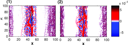
Figure 1: (Color online) Snapshots of two realizations of the WF for $N=101$ and DOD with $\Delta=1/2$ at time $t=40$.

There appear non-vanishing values of the WF at nodes opposite to the initial node $j$, i.e., at $x\approx j+N/2$, even at infinitesimal small times $t$. These values are not related to disorder but are due to the PBCs. This can be inferred from Eq. (3). Consider first the case of even $N$: for $t=0$ and $x=j$ the only contributions to the sum in Eq. (3) are those for which $y=0$. However, for $t=0$ and also for $x=j+N/2$ the WF does not vanish: There are non-zero contributions to the sum for $y=N/2$, since we have $\langle j|j\rangle\langle j|j+N\rangle=\langle j|j\rangle\langle j|j\rangle=1$. Non-zero values of the WF for $x=j+N/2$ continue to show up at later times, see also Mülken and Blumen (2006). The argumentation for odd $N$ is similar: Here, however, non-vanishing values at $x\approx j+N/2$ start to appear as soon as the wave function $\langle x|j;t\rangle$ spreads over more than one node. The difference between these non-vanishing WF-values for even and for odd $N$ at short times tends to zero as $1/N$ for $N$ large. We remark that the appearence of these non-vanishing WF-values for short times at $x\approx j+N/2$ does not lead to a finite transition probability $\pi_{j+N/2,j}(t)$, since at small $t$ the sum in Eq.(4) practically vanishes. This is in line with the situation for open boundaries, where the transition probabilities $\pi_{j+N/2,j}(t)$ also vanish at short times. There, however, also the WF-values at $x\approx j+N/2$ are practically zero at short times. A thorough study of the influence of different boundary conditions on the WF is beyond the scope of this paper and will be given elsewhere.

Once we have the WF, we also compute its long time average. Now it is preferrable not to first evaluate Eq. (7) and to perform then the computationally expensive time integrals of Eq. (5), but to proceed at first analytically, obtaining

$${\overline{W}}_{j}(x,\kappa) = \frac{1}{N}\sum_{y}e^{iky}\sum_{\theta,\theta^{\prime}}\tilde{\delta}(E_{\theta}-E_{\theta^{\prime}})$$ (8)

$$\times \langle x-y|\Phi_{\theta^{\prime}}\rangle\langle\Phi_{\theta^{\prime}}|j\rangle\langle j|\Phi_{\theta}\rangle\langle\Phi_{\theta}|x+y\rangle,$$

with $\tilde{\delta}(E_{\theta}-E_{\theta^{\prime}})=1$ if $E_{\theta}=E_{\theta^{\prime}}$ and $\tilde{\delta}(E_{\theta}-E_{\theta^{\prime}})=0$ otherwise. Eq. (8) is in general much more accurate and computationally cheaper.

IV.3 Ensemble averages

In order to have a global picture of the effect of disorder on the dynamics, we will consider ensemble averages of the WFs. For this we calculate the WF for different realizations of ${\bf H}$ and average over all realizations, i.e., for $R$ realizations we compute

$$\langle W_{j}(x,\kappa;t)\rangle_{R}\equiv\frac{1}{R}\sum_{r=1}^{R}\big{[}W_{j}(x,\kappa;t)\big{]}_{r},$$ (9)

where $\big{[}W_{j}(x,\kappa;t)\big{]}_{r}$ is the WF of the $r$th realization of ${\bf H}$.

V The role of disorder

For all cases of disorder, we study the WF for different strength of the disorder, i.e., for different $\Delta$ with $\Delta$ ranging from $\Delta=1/40$ to $\Delta=1/2$. We exemplify our results for odd ($N=101$) and even ($N=100$) numbered rings, where in all cases the initial condition ($t=0$) is a state localized at node $j$ (in our two examples $j=50$). Note that the WF of a localized state at $x=j$ is equipartitioned in the $\kappa$-direction, i.e., $W_{j}(j,\kappa;0)=1/N$.

V.1 Diagonal disorder (DD)

We start by considering diagonal disorder for a graph with $N=101$. Figure 2 shows snapshots of $\langle W_{j}(x,\kappa;t)\rangle_{R}$ for different values of $\Delta$ at different times.

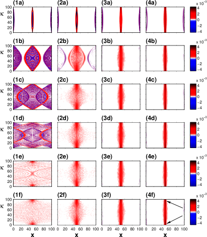
Figure 2: (Color online) DD: Ensemble average of WFs of the quantum dynamics on a ring of length $N=101$ for $\Delta=1/40,1/10,1/4$, and $1/2$ [columns (1)-(4)], each at times $t=1,10,20,40,100$, and $500$ [rows (a)-(f)]. The initial node is always $j=50$ and the average is over $R=1000$ realizations. Red regions denote positive values of the averaged WFs, blue regions negative values and white regions values close to $0$. The colormaps are always chosen to be the same for each row but might differ in different rows. The maximal values of $\langle W_{j}(x,\kappa;t)\rangle_{R}$ are denoted by small black regions; these are highlighted and exemplified by the arrows in panel (4f).

The first column shows $\langle W_{j}(x,\kappa;t)\rangle_{R}$ for $\Delta=1/40$ at times $t=1,10,20,40,100$, and $500$ [Fig. 2(1a)-(1f)]. For this quite weak disorder, the patterns in phase space are similar to the unperturbed case, where “waves” in phase space emanate from the initial site $x=j=50$ and start to interfere after having reached the opposite site of the ring (see Fig. 3 of Mülken and Blumen (2006)). However, at longer times differences become visible, Fig 2(1f). The pattern for the unperturbed case is quite irregular but with alternating positive and negative regions of the WF of approximately the same magnitude. Here, the disorder causes a decrease of $\langle W_{j}(x,\kappa;t)\rangle_{R}$ for $x$ close to the initial site $j=50$ and $\kappa$-values in the middle of the interval $[0,N-1]$ compared to the values of $\kappa$ close to $0$ or $N-1$.

Increasing the disorder parameter $\Delta$, the patterns change profoundly. The wave structure gets suppressed and for all $\kappa$ a localized region forms about the initial site $j=50$ already for small disorder ($\Delta=1/10$) and short times ($t=20$), see Fig. 2(2c).

For even larger values of $\Delta$, for all $\kappa$ the formation of a localized region about $j=50$ becomes even more pronounced. Already for $\Delta=1/4$ this localized region forms for times as short as $t=10$, see Fig. 2(3b). At $\Delta=1/2$, $\langle W_{j}(x,\kappa;t)\rangle_{R}$ stays localized for all times [Fig. 2(4a)-(4f)]. Also here, values of the WF at about $\kappa\approx N/2$ are decreased, whereas values of the WF for $\kappa$ about the interval borders $0$ and $N-1$ remain rather large for $x\approx j$, as indicated by the thin black region (see also the arrows), e.g., in Fig. 2(4f). We further note that at high disorder the localized averaged WF is always positive, i.e., all fluctuations, present for small disorder, have vanished. We recall that the WF is normalized to one when integrated over the whole phase space.

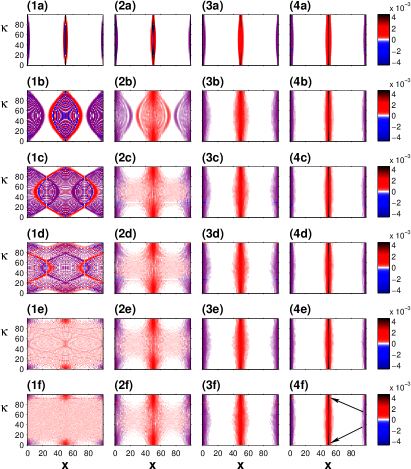
Figure 3: (Color online) DD: Same as Fig. 2 but for $N=100$.

Having an even number of nodes in the graph does not alter the picture drastically. By comparing Fig. 2 to Fig. 3, which shows the quantum dynamics on a ring of $N=100$ nodes with DD, one sees that the corresponding panels are rather similar; the localization effect of the disorder on the system stays the same. However, there are also differences at long times, compare (1e-f) and (2e-f) in each figure. Another difference between even and odd $N$ lies in the fact that for even $N$ there remains a region of alternating values of $\langle W_{j}(x,\kappa;t)\rangle_{R}$ at about $x=j+N/2$, even for large disorder, see column (4a)-(4f). This is due to the periodic boundary condition and, therefore, to the equal number of steps in both directions starting from any site on the network needed to reach the opposite site of the network. Obviously, the disorder does not destroy this symmetry.

V.2 Diagonal and off-diagonal disorder (DOD)

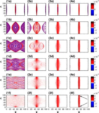
Figure 4: (Color online) DOD: Same values of $t$, $\Delta$, and $R$ as used in Fig. 2.

The second type of disorder is the diagonal and off-diagonal one (DOD), where both the diagonal and the off-diagonal elements of the unperturbed Hamiltonian are randomly changed, as explained in Sec. II.2. Figure 4 shows $\langle W_{j}(x,\kappa;t)\rangle_{R}$ for the same values of $t$, $\Delta$, and $R$ as in Fig. 2. Here and as for DD, the symmetry with respect to the line in phase space at $x=j=50$ remains intact. Comparing to the DD case, there is a slightly weaker suppression of the waves in phase space. This effect is rather small but can be seen by comparing, e.g., the values of the WF in Fig. 2(2f) to the ones in Fig. 4(2f), note the different corresponding colorbars. However, the overall localization effect is very similar for both types of disorder.

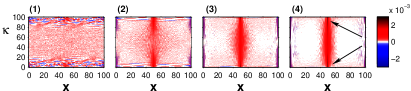
Figure 5: (Color online) Constrained diagonal and off-diagonal disorder, see text for details: Averaged WF for $N=101$ and $t=500$ [cases (f) in Figs. 2 to 4], but for the same values of $\Delta$ and $R$ as used in Fig. 2.

Another possibility is to constrain the disorder by having $2\Delta_{j,j}=\Delta_{j,j-1}+\Delta_{j,j+1}$, which maintains the connection of ${\bf H}$ to the classical transfer matrix ${\bf T}$. Figure 5 shows the WF evaluated in this way for $N=101$ at time $t=500$ and for $\Delta=1/40,~{}1/10,~{}1/4$ and $1/2$. Also here, the localization effect is clearly seen. Nevertheless, the details of the WF differ from those obtained for the other types of disorder.

VI Marginal distributions

Integrating the WF along lines in phase space gives the marginal distributions. Since we saw that the effect of localization does not depend on the particular choice of the type of disorder, we display the marginal distributions only for DOD. Figure 6 shows the marginal distributions for $N=101$ at time $t=100$ for different $\Delta$. Obviously, the details of the WF are lost when integrating along either the $x$ or the $\kappa$ direction.

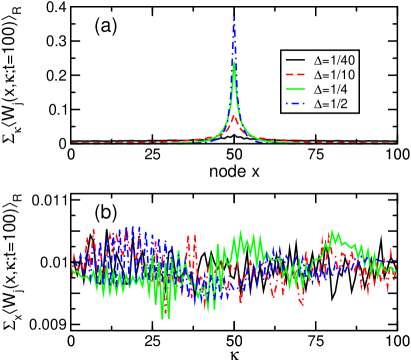
Figure 6: (Color online) DOD: Marginal distributions of $\left<W_{j}(x,\kappa;t)\right>_{R}$, for $N=101$ at $t=100$, for $\Delta=1/40,1/10,1/4$, and $1/2$. (a) summing along the $\kappa$ direction, (b) summing along the $x$ direction.

While the transition probabilities, obtained by summing over all $\kappa$ [Fig.6(a)], clearly show the effect of localization, this is not the case for the marginal distribution obtained by summing over all $x$ [Fig.6(b)]. In the latter case, one cannot readily distinguish the situations corresponding to different values of $\Delta$.

VII Long time averages

In has been shown in Mülken and Blumen (2006) that for unperturbed coherent exciton transport and odd $N$ (superscript ^o), most points in the quantum mechanical phase space have a weight of $1/N^{2}$, namely we have

$${\overline{W}}^{o}_{j}(x,\kappa)=\begin{cases}1/N^{2}&\kappa\neq 0\ \mbox{and any}\ x\\ 1/N&\kappa=0\ \mbox{and}\ x=j\\ 0&\mbox{else.}\end{cases}$$ (10)

For even $N$, the limiting WF reads

$${\overline{W}}^{e}_{j}(x,\kappa)=\begin{cases}2/N^{2}&\kappa\neq 0,\ \kappa\ \mbox{even}\ \mbox{and any}\ x\\ 1/N&\kappa=0\ \mbox{and}\ x=j,j+N/2\\ 0&\mbox{else.}\end{cases}$$ (11)

We note that Eq. (11) differs from Eq. (19) of Ref. Mülken and Blumen (2006), which is not correct. The long time averages of the WFs for even $N$ are somewhat peculiar, since values different from zero appear only for even $\kappa$, whereas the WFs themselves have values different from zero at arbitrary times for all $\kappa$. A numerical check (which we do not include here) for a finite line of $N$ nodes without disorder, shows that these stripes in the long time average in the present study are due to the periodic boundaries. For even $N$ there are constructive interference patterns in the transition probabilities, since the number of steps in both directions is the same, see also Ref. Mülken and Blumen (2005). For a finite line with even $N$, there are no stripes in the long time average. Of course, for short times and close to the initial node, the WFs for the line and the circle coincide, since the boundaries have no effect on the initial propagation. Nevertheless, one also has to bear in mind that the long time average is not a real equilibrium distribution.

As a technical note, we remark that changing the order of the time and ensemble averages can lead to a considerable speed-up of the numerical computation. We checked numerically that the time average and the ensemble average indeed interchange, i.e., we have

$$\langle{\overline{W}}_{j}(x,\kappa)\rangle_{R} \equiv \Big{\langle}\lim_{T\to\infty}\frac{1}{T}\int\limits_{0}^{T}dt\ W_{j}(x,\kappa;t)\Big{\rangle}_{R}$$ (12)

$$= \lim_{T\to\infty}\frac{1}{T}\int\limits_{0}^{T}dt\ \langle W_{j}(x,\kappa;t)\rangle_{R}.$$

Now, using Eq. (8) reduces the computational effort further. For computational reasons, we further interchanged the summation over $y$ with the ensemble average, i.e.,

$$\langle{\overline{W}}_{j}(x,\kappa)\rangle_{R}=\Big{\langle}\frac{1}{N}\sum_{y}e^{iky}\sum_{\theta,\theta^{\prime}}\tilde{\delta}(E_{\theta}-E_{\theta^{\prime}})$$

$$\qquad\times\langle x-y|\Phi_{\theta^{\prime}}\rangle\langle\Phi_{\theta^{\prime}}|j\rangle\langle j|\Phi_{\theta}\rangle\langle\Phi_{\theta}|x+y\rangle\Big{\rangle}_{R}$$

$$=\frac{1}{N}\sum_{y}e^{iky}\Big{\langle}\sum_{\theta,\theta^{\prime}}\tilde{\delta}(E_{\theta}-E_{\theta^{\prime}})$$

$$\qquad\times\langle x-y|\Phi_{\theta^{\prime}}\rangle\langle\Phi_{\theta^{\prime}}|j\rangle\langle j|\Phi_{\theta}\rangle\langle\Phi_{\theta}|x+y\rangle\Big{\rangle}_{R}.$$ (13)

Again, we carefully checked that Eq. (13) yields the same result as Eq. (12).

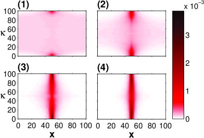
Figure 7: (Color online) DOD: Limiting averaged WF, $\langle{\overline{W}}_{j}(x,\kappa)\rangle_{R}$, for $N=101$ and $\Delta=1/40$, $1/10$, $1/4$, and $1/2$ [panels (1) to (4), respectively], according to Eq.(13).

Now, the disorder changes also the limiting WF quite drastically. Starting from high disorder of $\Delta=1/2$, we expect from Figs. 2(4a)-(4f) to 4(4a)-(4f) that the long time average of the averaged WF will look basically the same. Figure 7 shows the limiting averaged WF for $N=101$ and DOD according to Eq. (13). Indeed, for large $\Delta$, the limiting averaged WF is comparable to the corresponding averaged WF, compare Figs. 7(4) and 4(4f). Close to the initial node $x=j=50$ and there along the $\kappa$-direction, $\langle{\overline{W}}_{j}(x,\kappa)\rangle_{R}$ has large (positive) values for $\kappa$ about $0$ and $N-1$ which decrease by going toward $\kappa=N/2$. Here, the minimum of this decrease depends on the particular type of disorder.

Also for small $\Delta$ there are significant differences to the case without disorder. From Fig. 7(1) we see that the disorder “smears out” the localized value $\overline{W}_{j}(j,0)=1/N$ in the case without disorder, see Eq.(10). Specifically, the $(x=j,\kappa=0)$-value decreases while the neighboring ones increase. For $\Delta=1/10$, the onset of localization about $x=j=50$ is already seen, see Fig. 7(2), and becomes more and more pronounced as $\Delta$ increases, Fig. 7(3). Furthermore, all other values of $\langle{\overline{W}}_{j}(x,\kappa)\rangle_{R}$ for $x\neq j$ decrease with increasing disorder, as can be seen by the decreasing size of the light pink region, which corresponds to values close to $1/N^{2}$. In fact, the values of the limiting averaged WF for $x$ distant from $x=j=50$ drop to zero, shown as white regions in Fig. 7.

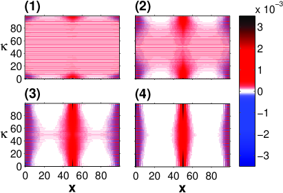
Figure 8: (Color online) Same as Fig. 7 but for $N=100$.

For even $N$ we found that without disorder the limiting WF shows a peculiar “striped” distribution, caused by the PBCs, see Eq.(11). By switching on the disorder, these peculiarities vanish. Figure 8 shows the limiting averaged WF for DOD and $N=100$. Although for small $\Delta$ there are some remainders of stripes left, these disappear completely for higher values of $\Delta$, compare Figs. 8(1)-(4). Note further that the second peak of ${\overline{W}}^{e}_{j}(x,\kappa)$ at $x=j+N/2$, see Eq.(11), transforms for increasing disorder to an oscillatory line in the $\kappa$-direction at $x=j+N/2$.

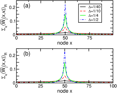
Figure 9: (Color online) DOD: Marginal distribution $\sum_{\kappa}\langle{\overline{W}}_{j}(x,\kappa)\rangle_{R}$ for different $\Delta$ and (a) $N=100$ and (b) $N=101$.

By summing now again along the $\kappa$-direction, this peculiar behavior vanishes and also for even $N$ we get a localized marginal limiting probability distribution at $x=j$. Figure 9 shows the marginal distribution $\sum_{\kappa}\langle{\overline{W}}_{j}(x,\kappa)\rangle_{R}$ for even and odd $N$ with DOD. As expected, for even $N$, Fig. 9(a), there are no remainders of the peculiar distribution of $\langle{\overline{W}}_{j}(x,\kappa)\rangle_{R}$ at $x=j+N/2$ for large $\Delta$. Furthermore, for high disorder, the marginal distributions of $\langle{\overline{W}}_{j}(x,\kappa)\rangle_{R}$ have a shape similar to that of $\langle W_{j}(x,\kappa,t)\rangle_{R}$, compare Figs. 6(a) and 9(b).

In general, the difference in the long time average $\sum_{\kappa}\langle{\overline{W}}_{j}(x,\kappa)\rangle_{R}$ between even and odd $N$ strongly depends on the disorder. Without disorder, the two cases are distinct Mülken and Blumen (2006). For odd $N$ the constructive interference at the node $j$ leads to only one peak in $\sum_{\kappa}\langle{\overline{W}}_{j}(x,\kappa)\rangle_{R}$, see Eq. (20) in Mülken and Blumen (2006). However, for even $N$ the constructive interference at nodes $j$ and also at node $j+N/2$ leads to two peaks in $\sum_{\kappa}\langle{\overline{W}}_{j}(x,\kappa)\rangle_{R}$, see Eq. (21) in Mülken and Blumen (2006). With increasing disorder, the second peak in $\sum_{\kappa}\langle{\overline{W}}_{j}(x,\kappa)\rangle_{R}$ for even $N$ at $x=j+N/2$ vanishes and gives rise to only one peak at $x=j$, see Fig. 9. Nonetheless, for large but finite $N$ the WF itself [given in Eq.(3)] still allows us to distinguish between the odd and the even case, see Figs. 7 and 8.

VIII Conclusions

We have analyzed the effect of static disorder on the coherent exciton transport by means of discrete Wigner functions. We have studied numerically the dynamics on a ring of $N$ sites in the presence of pure diagonal disorder and also of diagonal and off-diagonal disorder. The previously found characteristic patterns of the unperturbed WF in the quantum mechanical phase space are destroyed by the disorder. Instead, the WF shows strong localization about the initial node. Integrating out the details of the time evolution by considering the long time average of the WF, shows an even more pronounced localization.

References

- Wigner (1932) E. P. Wigner, Phys. Rev. 40, 749 (1932).
- Hillery et al. (1984) M. Hillery, R. F. O’Connell, M. O. Scully, and E. P. Wigner, Phys. Rep. 106, 121 (1984).
- Schleich (2001) W. P. Schleich, Quantum Optics in Phase Space (Wiley-VCH, Berlin, 2001).
- Mandel and Wolf (1995) L. Mandel and E. Wolf, Optical Coherence and Quantum Optics (Cambridge University Press, Cambridge, England, 1995).
- Kluksdahl et al. (1989) N. C. Kluksdahl, A. M. Kriman, D. K. Ferry, and C. Ringhofer, Phys. Rev. B 39, 7720 (1989).
- Buot (1993) F. A. Buot, Phys. Rep. 234, 73 (1993).
- Bordone et al. (1999) P. Bordone, M. Pascoli, R. Brunetti, A. Bertoni, C. Jacoboni, and A. Abramo, Phys. Rev. B 59, 3060 (1999).
- Anderson (1958) P. W. Anderson, Phys. Rev. 109, 1492 (1958).
- Abrahams et al. (1979) E. Abrahams, P. W. Anderson, D. C. Licciardello, and T. V. Ramakrishnan, Phys. Rev. Lett. 42, 673 (1979).
- Anderson (1978) P. W. Anderson, Rev. Mod. Phys. 50, 191 (1978).
- Logan and Wolynes (1987) D. E. Logan and P. G. Wolynes, J. Chem. Phys. 87, 7199 (1987).
- Abramavicius et al. (2004) D. Abramavicius, L. Valkunas, and R. van Grondelle, Phys. Chem. Chem. Phys. 6, 3097 (2004).
- Dominguez-Adame and Malyshev (2004) F. Dominguez-Adame and V. A. Malyshev, Am. J. Phys. 72, 226 (2004).
- Helmes et al. (2005) R. W. Helmes, M. Sindel, L. Borda, and J. von Delft, Phys. Rev. B 72, 125301 (2005).
- Barford and Duffy (2006) W. Barford and C. D. P. Duffy, Phys. Rev. B 74, 075207 (2006).
- Keating et al. (2006) J. P. Keating, N. Linden, J. C. F. Matthews, and A. Winter, arXiv: quant–ph/0606205 (2006).
- Farhi and Gutmann (1998) E. Farhi and S. Gutmann, Phys. Rev. A 58, 915 (1998).
- Mülken et al. (2006) O. Mülken, V. Bierbaum, and A. Blumen, J. Chem. Phys. 124, 124905 (2006).
- Kenkre and Reineker (1982) V. M. Kenkre and P. Reineker, Exciton Dynamics in Molecular Crystals and Aggregates (Springer, Berlin, 1982).
- Shore (1990) B. W. Shore, The Theory of Coherent Atomic Excitation (Wiley, New York, 1990).
- Haken (1976) H. Haken, Quantum Field Theory of Solids (North-Holland, Amsterdam, 1976).
- Mülken and Blumen (2006) O. Mülken and A. Blumen, Phys. Rev. A 73, 012105 (2006).
- Mülken and Blumen (2005) O. Mülken and A. Blumen, Phys. Rev. E 71, 036128 (2005).
- Wootters (1987) W. K. Wootters, Ann. Phys. 176, 1 (1987).
- Cohendet et al. (1988) O. Cohendet, P. Combe, M. Sirugeu, and M. Sirugue-Collin, J. Phys. A 21, 2875 (1988).
- Leonhardt (1995) U. Leonhardt, Phys. Rev. Lett. 74, 4101 (1995).
- Takami et al. (2001) A. Takami, T. Hashimoto, M. Horibe, and A. Hayashi, Phys. Rev. A 64, 032114 (2001).
- Miquel et al. (2002) C. Miquel, J. P. Paz, and M. Saraceno, Phys. Rev. A 65, 062309 (2002).