Truncated states obtained by iteration

Abstract

Quantum states of the electromagnetic field are of considerable importance, finding potential application in various areas of physics, as diverse as solid state physics, quantum communication and cosmology. In this paper we introduce the concept of truncated states obtained via iterative processes (TSI) and study its statistical features, making an analogy with dynamical systems theory (DST). As a specific example, we have studied TSI for the doubling and the logistic functions, which are standard functions in studying chaos. TSI for both the doubling and logistic functions exhibit certain similar patterns when their statistical features are compared from the point of view of DST. A general method to engineer TSI in the running-wave domain is employed, which includes the errors due to the nonidealities of detectors and photocounts.

I Introduction

Quantum state engineering is an area of growing importance in quantum optics, its relevance lying mainly in the potential applications in other areas of physics, such as quantum teleportation bennett93 , quantum computation Kane98 , quantum communication Pellizzari97 , quantum cryptography Gisin02 , quantum lithography Bjork01 , decoherence of states Zurek91 , and so on. To give a few examples of their usefulness and relevance, quantum states arise in the study of quantum decoherence effects in mesoscopic fields harochegato ; entangled states and quantum correlations brune ; interference in phase space bennett2 ; collapses and revivals of atomic inversion narozhny ; engineering of (quantum state) reservoirs zoller ; etc. Also, it is worth mentioning the importance of the statistical properties of one state in determining some relevant properties of another barnett , as well as the use of specific quantum states as input to engineer a desired state serra .

Dynamical Systems Theory (DST), on the other hand, is a completely different area of study, whose interest lies mainly in nonlinear phenomena, the source of chaotic phenomena. DST groups several approaches to the study of chaos, involving Lyapunov exponent, fractal dimension, bifurcation, and symbolic dynamics among other elements devaney . Recently, other approaches have been considered, such as information dynamics and entropic chaos degree ohya .

The purpose of this paper is twofold: to introduce novel states of electromagnetic fields, namely truncated states having coefficients obtained via iterative process (TSI), and to study chaos phenomena using standard techniques from quantum optics, making an analogy with DST. We note that, unlike previous states studied in the literature dodonov , each coefficient of the TSI is obtained from the previous one by iteration of a function. Features of this state are studied by analyzing several of its statistical properties in different regimes (chaotic versus nonchaotic) according to DST, and, for some iterating functions, we found properties of TSI very sensitive (resembling chaos) to the first coefficient $C_{0}$, which is used as a   seed   to obtain the remaining $C_{n}$.

This paper is organized as follows. In section 2 we introduce the TSI and in section 3 we analyze the behavior of some of its properties as the Hilbert space dimension is increased. In section 4 we show how to engineer the TSI in the running-wave field domain, and the corresponding engineering fidelity is studied in section 5. In section 6 we present our conclusions.

II Truncated states obtained via iteration (TSI)

We define TSI as

$$|TSI\rangle=\sum\limits_{n=0}^{N}C_{n}|n\rangle$$ (1)

where $C_{n}$ is the normalized complex coefficient obtained as the $n$th iteration of a previously given generating function. For example, given $C_{0}$,$C_{n}$ can be the $n$th iterate of the quadratic functions: $C_{n}(\mu)=C_{n-1}^{2}+\mu$; sine functions: $C_{n}(\mu)=\mu\sin(C_{n-1})$; logistic functions $C_{n}(\mu)=\mu C_{n-1}(1-C_{n-1})$; exponential functions: $C_{n}=\mu\exp(C_{n-1})$; doubling function defined on the interval [0,1): $C_{n}=2C_{n-1}$ mod $1$, and so on, $\mu$ being a parameter. It is worth recalling that all the functions in the above list are familiar to researchers in the field of dynamical systems theory (DST). For example, for some values of $\mu$, it is known that some of these functions can behave in quite a chaotic manner devaney . Also, note that by computing all the $C_{n}$ we are in fact determining the orbit of a given function, and because the $C_{n}$ and $P_{n}$, the photon number distribution, are related by $P_{n}=|C_{n}|^{2}$, fixed or periodic points of a function will correspond to fixed or periodic $P_{n}$. Rather than studying all the functions listed in this section, we will focus on the doubling function and the logistic function. These two functions have been widely used to understand chaos in nature. As we shall see in the following, although very different from each other, these functions give rise to different TSI having similar patterns.

III Statistical properties of TSI using the doubling and the logistic functions

III.1 Photon Number Distribution

Since the expansion of TSI is known in the number state $|n\rangle$, we have

$$P_{n}=|C_{n}|^{2}.$$ (2)

Figs. $1$ and $2$ show the plots of the photon-number distribution $P_{n}$ versus $n$ for TSI using the doubling function. The Hilbert space dimension is $N=50$. In order to illuminate the behavior of TSI for different values of $C_{0}$, we take $C_{0}$ as $0.3$ and $0.29711$, respectively shown in Figs. $1$ and $2$. Note the regular behavior for $C_{0}=0.3$ and rather an irregular, or chaotic, behavior for $C_{0}=$ $0.29711$. Figs. $3$ and $4$ show $P_{n}$ for the logistic function. For $C_{0}=0.2$ and $\mu=3.49$ the logistic function behaves regularly (Fig.$3$), showing clearly (as in the case of the doubling-function) four values for $P_{n}$; by contrast, for $\mu=4$ and $C_{0}=0.2$, $P_{n}$ oscillates quite irregularly (Fig.$4$). This is so because the photon number distribution is equivalent to the orbit of the TSI dynamics devaney . Thus, once a fixed - attracting or periodic - point is attained, the subsequent coefficients, and hence the subsequent $P_{n}$, will behave in a regular manner. Conversely, when no fixed point exists, $P_{n}$ will oscillate in a chaotic manner. Therefore, by choosing suitable $C_{0}$ and/or $\mu$, we can compare the properties of TSI when different regimes (chaotic versus nonchaotic) in the DST sense are encountered. Note the similarity between the properties of the logistic and the doubling functions when the DST regimes are the same. Interestingly, these similarities are observed when other properties are analyzed, as we shall see in the following.

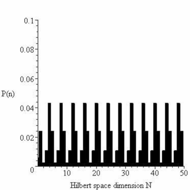
Figure 1: Photon number distribution for the doubling function with $C_{0}=0.3$. Note a four-period type for the probabilities; this regular behavior coincides with nonchaotic behavior of the doubling function in the DST sense.

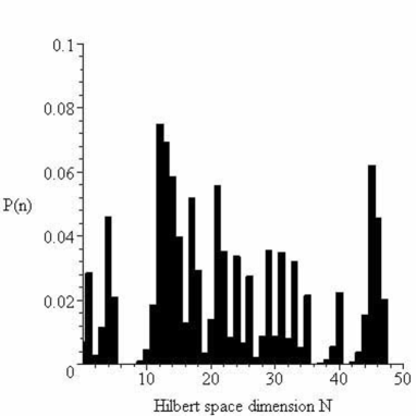
Figure 2: Photon number distribution for the doubling function with $C_{0}=0.29711$. This irregular behavior for $P_{n}$ coincides with the chaotic behavior of the doubling function in the DST sense.

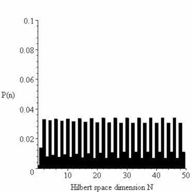
Figure 3: Photon number distribution for the logistic function with $C_{0}=0.2$ and $\mu=3.49$. This regular or “four-period” type behavior for the probabilities coincides with nonchaotic behavior in the DST sense.

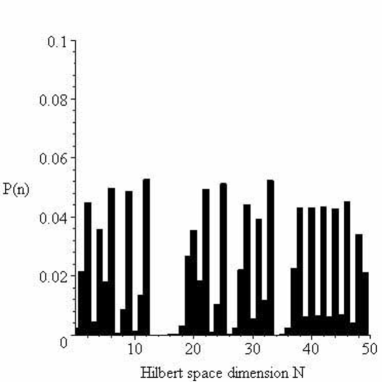
Figure 4: Photon number distribution for the logistic function with $C_{0}=0.2$ and $\mu=4$. This irregular behavior of $P_{n}$ coincides with the chaotic behavior of the logistic function in the DST sense.

III.2 Even and Odd Photon number distribution

The functions $P_{odd}$ and $P_{even}$ represent the photon number distribution for $n$ $odd$ and $even$, respectively, given by Eq. (2). It is well established in quantum optics Mandel that if $P_{odd}>0.5$ the Glauber-Sudarshan $P$-function assumes negative values, prohibited in the usual probability distribution function, and the quantum state has no classical analog. Since $P_{odd}+P_{even}=1$, the same is true when $P_{even}<0.5$ . Figs. $5$ and $6$ show the behavior of $P_{odd}$ for $C_{0}=0.3$ and $C_{0}=0.29711$ for the doubling function the Hilbert space $N$ is increased. Figs. $7$ and $8$ refer to the the logistic function for $\mu=3.49$ and $\mu=4$. In Figs. $5$ and $7$ (corresponding to a nonchaotic regime in DST), note that TSI has a classical analog as $N$ increases. From Figs. $6$ and $8$ (corresponding to a chaotic regime in DST), TSI can behave as a nonclassical state, depending on $N$. More interestingly, note the following pattern: whenever the coefficients of TSI correspond to the nonchaotic regime in DST, $P_{odd}$ (and so $P_{even}$) will remain above or below $0.5$ on a nearly monotonic curve, as seen in Figs. $5$ and $7$; whenever the coefficients of TSI correspond to the chaotic regime in DST, $P_{odd}$ (and so $P_{even}$) will tend to oscillate around $0.5$ (Figs. $6$ and $8$).

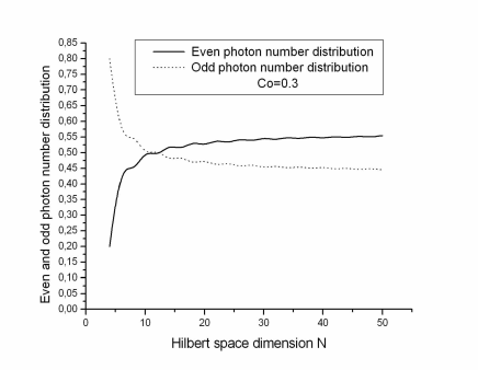
Figure 5: Even (solid) and odd (dots) photon number distributions for the doubling function. We have used $C_{0}=0.3$ to coincide with nonchaotic behavior in the DST sense.

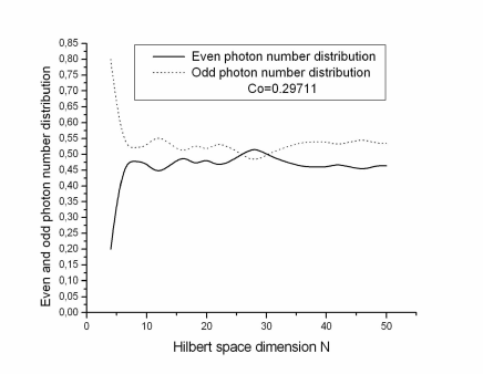
Figure 6: Even (solid) and odd (dots) photon number distributions for the doubling function. $C_{0}=0.29711$ was chosen to coincide with chaotic behavior in the DST sense.

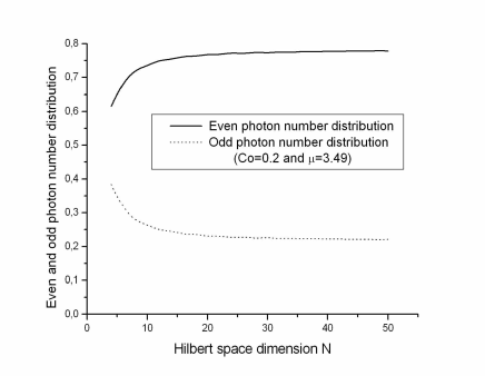
Figure 7: Even (solid) and odd (dots) photon number distributions for the logistic function. Here we chose $C_{0}=0.2$ and $\mu=3.49$ to coincide with nonchaotic behavior in the DST sense.

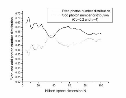
Figure 8: Even (solid) and odd (dots) photon number distributions for the logistic function. Here we chose $C_{0}=0.2$ and $\mu=4$ to coincide with chaotic behavior in the DST sense.

III.3 Average number and variance

The average number $\left\langle\hat{n}\right\rangle$ and the variance $\left\langle\Delta\hat{n}\right\rangle$ in TSI are obtained straightforwardly from

$$\left\langle\hat{n}\right\rangle=\sum_{n=0}^{N}P(n)n,$$ (3)

and

$$\left\langle\Delta\hat{n}\right\rangle=\sqrt{\left\langle\hat{n}^{2}\right\rangle-\left\langle\hat{n}\right\rangle^{2}}.$$

Fig. $9$ shows the plot of $\left\langle\hat{n}\right\rangle$ and Fig. $10$ the plot of $\left\langle\Delta\hat{n}\right\rangle$ as functions of the dimension $N$ of Hilbert space, for the doubling function. Note the near linear behavior of the average photon number and its variance as $N$ increases for $C_{0}=0.3$ (nonchaotic regime in DST); this is not seen when $C_{0}=0.29711$ (chaotic regime in DST). Figs. $11$ and $12$ for the logistic function show essentially the same behavior when these two DST regimes are shown together.

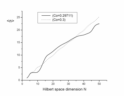
Figure 9: Average photon number for the doubling function. Here we chose $C_{0}=0.3$ (dots) and $C_{0}=0.29711$ (solid), allowing the Hilbert space $N$ to increase to $50$.

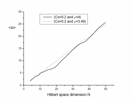
Figure 10: Variance of the photon number for the doubling function. Here we chose $C_{0}=0.3$ (dots) as well as $C_{0}=0.29711$(solid), allowing the Hilbert space $N$ to increase to $50$.

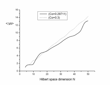
Figure 11: Average photon number for the logistic function. Here we chose $C_{0}=0.2$ with $\mu=3.49$ (dots) or $\mu=4$ (solid), allowing the Hilbert space $N$ to increase to $50$.

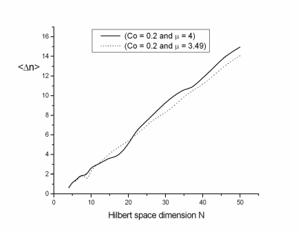
Figure 12: Variance of the photon number for the logistic function. Here we chose $C_{0}=0.2$ with $\mu=3.49$ (dots) or $\mu=4$ (solid), allowing the Hilbert space $N$ to increase to $50$.

III.4 Mandel parameter and second order correlation function

The Mandel $Q$ parameter is defined as

$$Q=\frac{\left(\Delta\hat{n}^{2}-\left\langle\hat{n}\right\rangle\right)}{\left\langle\hat{n}\right\rangle},$$ (4)

while the second order correlation function $g^{\left(2\right)}(0)$ is

$$g^{\left(2\right)}(0)=\frac{\left(\left\langle\hat{n}^{2}\right\rangle-\left\langle\hat{n}\right\rangle\right)}{\left\langle\hat{n}\right\rangle^{2}},$$

and for $Q<0$ ($Q>0$) the state is said to be sub-Poissonian (super-Poissonian). Also, the $Q$ parameter and the second order correlation function $g^{\left(2\right)}$ are related by walls

$$Q=\left[g^{\left(2\right)}(0)-1\right]\left\langle\hat{n}\right\rangle.$$ (5)

If $g^{\left(2\right)}(0)<0$, then the Glauber-Sudarshan $P$-function assumes negative values, outside the range of the usual probability distribution function. Moreover, by Eq. (5) it is readily seen that $g^{\left(2\right)}(0)<1$ implies $Q<0$. As for a coherent state $Q=0$, a given state is said to be a “classical” one if $Q>0$.

Figs. $13$ to $16$ show the plots of the $Q$ parameter and the correlation function $g^{\left(2\right)}(0)$ versus $N$ , for both the doubling and the logistic functions. Note that TSI is predominantly super-Poissonian for these two functions ($Q>0$ and $g^{\left(2\right)}(0\dot{)}>1$), thus being a “classical” state in this sense for $N\gtrsim 12$, while for small values of  $N$ ($N<12$), the $Q$ parameter is less than $0$, showing sub-Poissonian statistics and is thus associated with a “quantum state”. From Figs.$13$ and $15$, note that using $C_{0}=0.3$ for the doubling function, $C_{0}=0.2$ and $\mu=3.49$ for the logistic function (nonchaotic regime in DST), $Q$ shows a linear dependence on $N$. However, using $C_{0}=0.29711$ for the doubling function, $C_{0}=0.2$ and $\mu=4$ for the logistic function (chaotic regime in DST), $Q$ oscillates irregularly. Similarly, from Figs. $14$ and $16$, using $C_{0}=0.3$ for the doubling function, $C_{0}=0.2$ and $\mu=3.49$ for the logistic function, we see that $g^{\left(2\right)}(0)$ increases smoothly, while using $C_{0}=0.29711$ for the doubling function, $C_{0}=0.2$ and $\mu=4$ for the logistic function, the rise of $g^{\left(2\right)}(0)$ is rather irregular. This pattern is observed for other $C_{0}$ as input as well as for other values of the parameter $\mu$, and whenever the dynamics is chaotic (regular), the $Q$ parameter and the $g^{\left(2\right)}(0)$ correlation function oscillate irregularly (regularly).

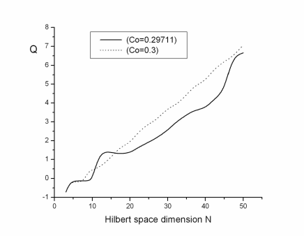
Figure 13: Q parameter for the doubling function. Here we chose $C_{0}=0.3$ (dots)  and $C_{0}=0.29711$ (solid), allowing the Hilbert space $N$ to increase to $50$. Note the irregular behavior of the Q parameter when $C_{0}=0.29711$, coinciding with chaotic behavior in the DST sense.

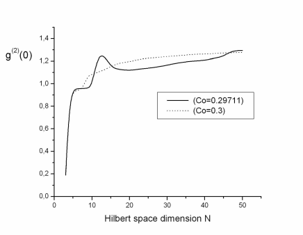
Figure 14: Second order correlation function for the doubling function. Here we chose $C_{0}=0.3$ (dots) and $C_{0}=0.29711$ (solid), allowing the Hilbert space $N$ to increase to $50$. Note the irregular rise of the $g(0)$ function when $C_{0}=0.29711$, coinciding with chaotic behavior in the DST sense.

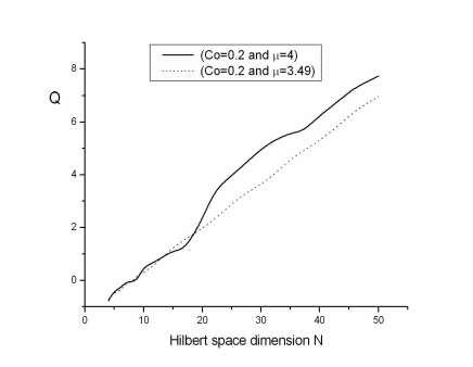
Figure 15: Q parameter for the logistic function. Here we chose $C_{0}=0.2$, with $\mu=3.49$ (dots) and $\mu=4$ (solid), allowing the Hilbert space $N$ to increase up to $50$. Note the irregular behavior of the Q parameter when $\mu=4$, exactly when chaotic behavior occurs according to DST.

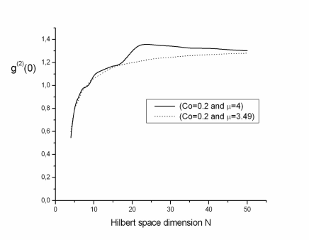
Figure 16: Second order correlation function for the logistic function. Here we chose $C_{0}=0.2$, with $\mu=3.49$ (dots) and $\mu=4$ (solid), allowing the Hilbert space $N$ to increase up to $50$. Note the irregular rise of $g^{2}(0)$ when $\mu=4$, exactly when chaotic behavior occurs according to DST.

III.5 Quadrature and variance

Quadrature operators are defined as

$$X_{1} =\frac{1}{2}\left(a+a^{\dagger}\right);$$

$$X_{2} =\frac{1}{2i}\left(a-a^{\dagger}\right).$$ (6)

where $a$ ($a^{\dagger}$)  is the annihilation (creation) operator in Fock space. Quantum effects arise when the variance of one of the two quadratures attains a value $\Delta X_{i}<0.5$, $i=1,2$. Figs. $17$ and $18$ show the plots of quadrature variance $\Delta X_{i}$ versus $N$. Note in this figures that variances increase when $N$ is increased.

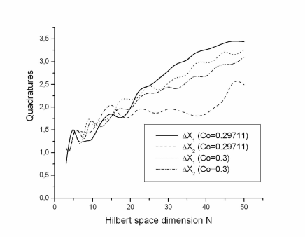
Figure 17: Averaged quadratures for the doubling function when the Hilbert space $N$ is increased to $50$. Doted (dashed-doted) line refer to quadrature variance $1$ $(2)$ for $C_{0}=0.3$; solid (dashed) line refer to quadrature variance 1 $(2)$ for $C_{0}=0.29711$.

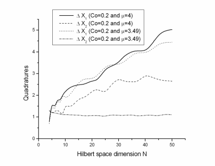
Figure 18: Averaged quadratures for the logistic function with $C_{0}=0.2$ when the Hilbert space N is increased to $50$. Doted (dashed-doted) line refer to quadrature variance $1$ ($2$) for $\mu=3.49$; solid (dashed) refer to quadrature variance 1 ($2$) for $\mu=4$.

III.6 Husimi -Q function

The Husimi Q-function for TSI is given by

$$Q_{\left|TSI\right\rangle}(\beta)=\frac{1}{\pi}\left|\left\langle\beta|TSI\right\rangle\right|^{2},$$ (7)

where $\beta$ is a coherent state. Figs. $19$ to $22$ show the Husimi Q-function for both the doubling and the logistic functions for $N=15.$ For the doubling function, we use $C_{0}=0.29711$ and $C_{0}=0.3$, respectively, and for the logistic function we use $\mu=3.49$ and $\mu=4$, respectively, for the chaotic and nonchaotic regimes. Interestingly, even when the chaotic and nonchaotic regimes of the DST are compared, Husimi Q-functions show essentially no difference from each other.

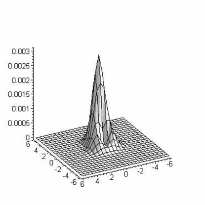
Figure 19: Husimi Q function for doubling function. Here $C_{0}=0.3$.

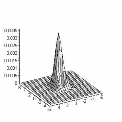
Figure 20: Husimi Q function for doubling function. Here $C_{0}=0.29711$.

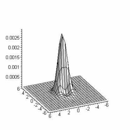
Figure 21: Husimi Q function for logistic function. Here $C_{0}=0.2$ and $\mu=3.49$.

Figure 22: Husimi Q function for logistic function. Here $C_{0}=0.2$ and $\mu=4$.

IV Generation of TSI

TSI can be generated in various contexts, as for example trapped ions serra2 , cavity QED serra ; vogel , and travelling wave-fields dakna . But due to severe limitation imposed by coherence loss and damping, we will employ the scheme introduced by Dakna et al. dakna in the realm of running wave field. For brevity, the present application only shows the relevant steps of Ref.dakna , where the reader will find more details. In this scheme, a desired state $\left|\Psi\right\rangle$ composed of a finite number of Fock states $\left|n\right\rangle$ can be written as

$$\left|\Psi\right\rangle = \sum_{n=0}^{N}C_{n}\left|n\right\rangle=\frac{C_{N}}{\sqrt{N!}}\prod_{n=1}^{N}\left(\hat{a}^{+}-\beta_{n}^{\ast}\right)\left|0\right\rangle$$ (8)

$$= \frac{C_{N}}{\sqrt{N!}}\prod_{k=1}^{N}\hat{D}(\beta_{k})\hat{a}^{+}\hat{D}(\beta_{k})\left|0\right\rangle,$$

where $\hat{D}(\beta_{n})$ stands for the displacement operator and the $\beta_{n}$ are the roots of the polynomial equation

$$\sum\limits_{n=0}^{N}C_{n}\beta^{n}=0.$$ (9)

According to the experimental setup shown in the Fig.1 of Ref.dakna , we have (assuming $0$-photon registered in all detectors) that the outcome state is

$$\left|\Psi\right\rangle\sim\prod_{k=1}^{N}D(\alpha_{k+1})\hat{a}^{+}T^{\hat{n}}D(\alpha_{k})\left|0\right\rangle,$$ (10)

where $T$ is the transmittance of the beam splitter and ${\alpha}_{k}$ are experimental parameters. After some algebra, the Eq.(8) and Eq.(10) can be connected. In this way, one shows that they become identical when ${\alpha}_{1}=-\sum_{l=1}^{N}T^{-l}{\alpha}_{l+1}$ and $\alpha_{k}=T^{\ast N-k+1}(\beta_{k-1}-\beta_{k})$ for $k=2,3,4\ldots N$.  In the present case the coefficients $C_{n}$ are given by those of the TSI. The roots $\beta_{k}^{\ast}=\left|\beta_{k}\right|e^{-i\varphi_{\beta_{k}}}$ of the characteristic polynomial in Eq.(9) and the displacement parameters $\alpha_{k}=\left|\alpha_{k}\right|e^{-i\varphi_{\alpha_{k}}}$ are shown in the Tables I;II;III and IV, for $N=5.$

Table 1: The roots $\beta_{k}^{\ast}=|\beta_{k}|e^{-i\varphi_{\beta_{k}}}$ of the characteristic polynomial and the displacement parameters $\alpha_{k}^{\ast}=|\alpha_{k}|e^{-i\varphi_{\alpha_{k}}}$ are given for TSI using the doubling function for $C_{0}=0.3$ (coinciding with nonchaotic behavior in the DST sense), $N=5$ and $T=0.862$. The probability of producing the state is 0.22$\%.$

N $\left|\beta_{k}\right|$ $\varphi_{\beta_{k}}$ $\left|\alpha_{k}\right|$ $\varphi_{\alpha_{k}}$ 1 2.169 2.638 1.187 -0.220 2 2.169 -2.638 1.155 1.570 3 0.545 3.141 1.096 -2.483 4 1.460 1.084 1.323 -2.331 5 1.460 -1.084 2.225 1.570 6 1.460 -1.084

Table 2: The roots $\beta_{k}^{\ast}=|\beta_{k}|e^{-i\varphi_{\beta_{k}}}$ of the characteristic polynomial and the displacement parameters $\alpha_{k}^{\ast}=|\alpha_{k}|e^{-i\varphi_{\alpha_{k}}}$ are given for a TSI using the doubling function for $C_{0}=0.29711$ (coinciding with chaotic behavior in the DST sense), $N=5$ and $T=0.867$. The probability of producing the state is 0.21$\%$

N $\left|\beta_{k}\right|$ $\varphi_{\beta_{k}}$ $\left|\alpha_{k}\right|$ $\varphi_{\alpha_{k}}$ 1 2.306 2.692 1.372 -0.198 2 2.306 -2.692 1.130 1.570 3 0.543 3.141 1.193 -2.563 4 1.489 1.089 1.357 -2.321 5 1.489 -1.089 2.289 1.570 6 1.489 -1.089

Table 3: The roots $\beta_{k}^{\ast}=|\beta_{k}|e^{-i\varphi_{\beta_{k}}}$ of the characteristic polynomial and the displacement parameters $\alpha_{k}^{\ast}=|\alpha_{k}|e^{-i\varphi_{\alpha_{k}}}$ are given for TSI using the logistic function for $C_{0}=0.2$, $\mu=3.49$ (coinciding with nonchaotic behavior in the DST sense), $N=5$ and $T=0.893$. The probability of producing the state is 0.11$\%$

N $\left|\beta_{k}\right|$ $\varphi_{\beta_{k}}$ $\left|\alpha_{k}\right|$ $\varphi_{\alpha_{k}}$ 1 3.948 3.141 2.794 0.051 2 0.609 2.566 2.195 -3.045 3 0.609 -2.566 0.472 1.570 4 1.828 1.373 1.830 -1.959 5 1.828 -1.373 3.202 1.570 6 1.828 -1.373

Table 4: The roots $\beta_{k}^{\ast}=|\beta_{k}|e^{-i\varphi_{\beta_{k}}}$ of the characteristic polynomial and the displacement parameters $\alpha_{k}^{\ast}=|\alpha_{k}|e^{-i\varphi_{\alpha_{k}}}$ are given for TSI using the logistic function for $C_{0}=0.2,$ $\mu=4$ (coinciding with chaotic behavior in the DST sense), $N=5$ and $T=0.879$. The probability of producing the state is 0.15$\%$

N $\left|\beta_{k}\right|$ $\varphi_{\beta_{k}}$ $\left|\alpha_{k}\right|$ $\varphi_{\alpha_{k}}$ 1 3.290 3.141 2.027 0.094 2 0.563 2.708 1.665 -3.056 3 0.563 -2.708 0.321 1.570 4 1.893 1.255 1.787 -2.064 5 1.893 -1.255 3.165 1.570 6 1.893 -1.255

For $N=5$, the best probability of producing TSI is $0.22\%$ when the doubling function is used, and $\ 0.15\%$ when the logistic funcion is used. The beam-splitter transmittance which optimizes this probability is around $T=0.878$.

V Fidelity of generation of TSI

Until now we have assumed all detectors and beam-splitters as ideal. Although very good beam-splitters are available by advanced technology, the same is not true for photo-detectors in the optical domain. Thus, let us now take into account the quantum efficiency $\eta$ at the photodetectors. For this purpose, we use the Langevin operator technique as introduced in norton1 to obtain the fidelity to get the TSI.

Output operators accounting for the detection of a given field $\hat{\alpha}$ reaching the detectors are given by norton1

$$\widehat{\alpha}_{out}=\sqrt{\eta}\widehat{\alpha}_{in}+\widehat{L}_{\alpha},$$ (11)

where $\eta$ stands for the efficiency of the detector and $\widehat{L}_{\alpha}$, acting on the environment states, is the noise or Langevin operator associated with losses into the detectors placed in the path of modes $\widehat{\alpha}=a,b$. We assume that the detectors couple neither different modes $a,b$ nor the Langevin operators $\widehat{L}_{\alpha}$, so the following commutation relations are readily obtained from Eq.(11):

$$\left[\widehat{L}_{\alpha},\widehat{L}_{\alpha}^{\dagger}\right] = 1-\eta,$$ (12)

$$\left[\widehat{L}_{\alpha},\widehat{L}_{\beta}^{\dagger}\right] = 0.$$ (13)

The ground-state expectation values for pairs of Langevin operators are

$$\left\langle\widehat{L}_{\alpha}\widehat{L}_{\alpha}^{\dagger}\right\rangle = 1-\eta,$$ (14)

$$\left\langle\widehat{L}_{\alpha}\widehat{L}_{\beta}^{\dagger}\right\rangle = 0,$$ (15)

which are useful relations specially for optical frequencies, when the state of the environment can be very well approximated by the vacuum state, even for room temperature.

Let us now apply the scheme of the Ref.dakna to the present case. For simplicity we will assume all detectors having high efficiency ($\eta\gtrsim 0.9$). This assumption allows us to simplify the resulting expression by neglecting terms of order higher than $(1-\eta)^{2}$. When we do that, instead of $|TSI\rangle$, we find the (mixed) state $|\Psi_{FE}\rangle$ describing the field plus environment, the latter being due to losses coming from the nonunit efficiency detectors. We have,

$$\left|\Psi_{FE}\right\rangle \sim R^{N}D(\alpha_{N+1})\hat{a}^{\dagger}T^{\hat{n}}D(\alpha_{N})\hat{a}^{\dagger}T^{\hat{n}}$$ (16)

$$\times D(\alpha_{N-1})\ldots\hat{a}^{\dagger}T^{\hat{n}}D(\alpha_{1})\left|0\right\rangle\widehat{L}_{0}^{\dagger}$$

$$+ R^{N-1}D(\alpha_{N+1})\hat{a}^{\dagger}T^{\hat{n}}D(\alpha_{N})\hat{a}^{\dagger}T^{\hat{n}}$$

$$\times D(\alpha_{N-1})\ldots\widehat{L}_{1}^{\dagger}T^{\hat{n}}D(\alpha_{1})\left|0\right\rangle$$

$$+ R^{N-1}D(\alpha_{N+1})\hat{a}^{\dagger}T^{\hat{n}}D(\alpha_{N})\widehat{L}_{N-1}^{\dagger}T^{\hat{n}}$$

$$\times D(\alpha_{N-1})\ldots\hat{a}^{\dagger}T^{\hat{n}}D(\alpha_{1})\left|0\right\rangle$$

$$+ R^{N-1}D(\alpha_{N+1})\widehat{L}_{N}^{\dagger}T^{\hat{n}}D(\alpha_{N})\hat{a}^{\dagger}T^{\hat{n}}$$

$$\times D(\alpha_{N-1})\ldots\hat{a}^{\dagger}T^{\hat{n}}D(\alpha_{1})\left|0\right\rangle,$$

where, for brevity, we have omitted the kets corresponding to the environment. Here $R$ is the reflectance of the beam splitter, $\ \widehat{L}_{0}^{\dagger}=\mathbf{1}$ is the identity operator and $\widehat{L}_{k}$, $k=1,2..N$ stands for losses in the first, second $\ldots$ $N-th$ detector. Although the $\widehat{L}_{k}\prime s$ commute with any system operator, we have maintained the order above to keep clear the set of possibilities for photo absorption: the first term, which includes $\widehat{L}_{0}^{\dagger}=\mathbf{1}$, indicates the probability for nonabsorption; the second term, which include $\widehat{\mathsf{L}}_{1}^{+}$, indicates the probability for absorption in the first detector; and so on. Note that in case of absorption at the k-$th$ detector, the annihilation operator $a$ is replaced by the $\widehat{L}_{k}^{\dagger}$ creation Langevin operator. Other possibilities such as absorption in more than one detector lead to a probability of order lesser than $(1-\eta)^{2}$, which will be neglected.

Next, we have to compute the fidelity nota , $F=\left\|\left\langle\Psi\right.\left|\Psi_{FE}\right\rangle\right\|^{2}$, where $\left|\Psi\right\rangle$ is the ideal state given by Eq.(10), here corresponding to the TSI characterized by the parameters shown in Tables I-IV, and $\left|\Psi_{FE}\right\rangle$ is the state given in the Eq.(16). Assuming $\eta=$ $0.99$, $0.95$ and $0.90$ and starting with $C_{0}=0.3$ and $C_{0}=0.29711$ for the doubling function, we find $F\simeq 0.9983$, $0.9943$ and $0.9909$, respectively, and for the logistic function, starting with $C_{0}=0.2$, $\mu=3.49$ and $\mu=4$, we find $F\simeq 0.9986$, $0.9944$ and $0.9911$, respectively. These high fidelities show that efficiencies around $0.9$ lead to states whose degradation due to losses is not so dramatic for $N=5$.

VI Comments and conclusion

In this paper we have introduced new states of the quantized electromagnetic field, named truncated states with probability amplitudes obtained through iteration of a function (TSI). Although TSI can be building using various functions such as logistic, sine, exponential functions and so on, we have focused our attention on the doubling and the logistic functions, which, as is well known from dynamical systems theory, can exhibit a chaotic behavior in the interval (0,1]. To characterize the TSI for the doubling and logistic functions we have studied various of its features, including some statistical properties, as well as the behavior of these features when the dimension $N$ of Hilbert space is increased. Interesting, we found a transition from sub-poissonian statistics to super-poissonian statistics when $N$ is relatively small ($N\sim 12$). Besides, photon number distribution, which is analogous to concept of orbits in the study of the dynamic of maps, shows a regular or rather a “chaotic” behavior depending on existing or not fixed or periodic points in the function to be iterated. Interestingly enough, we have found a pattern when the properties of  TSI for logistic function are compared with that of TSI for the doubling function from the point of view of dynamical systems theory (DST). For example, as $P_{n}$ has an analog with orbits from DST, it is straightforward to identify repetitions (or periods) in $P_{n}$, if there are any, when the Hilbert space is increased. Surprisingly, although the doubling and the logistic function are different from each other, when other properties such as even and odd photon number distribution, the average number and its variance, the Mandel parameter and the second order correlation function were studied, they presented the same following pattern: if, from the point of view of DST, the coefficients of TSI for the doubling and the logistic function correspond to a nonchaotic (chaotic) regime, all those properties increases smoothly (irregularly) when the Hilbert space is increased.

VII Acknowledgments

NGA thanks CNPq, Brazilian agency, and VPG-Universidade Católica de Goiás, and WBC thanks CAPES, for partially supporting this work.

References

- (1) C. H. Bennett et al 1993 Phys. Rev. Lett. 70 1895.
- (2) B. E. Kane 1998 Nature 393 143, and references therein.
- (3) T. Pellizzari 1997 Phys. Rev. Lett. 79 5242, and references therein.
- (4) N. Gisin, G. Ribordy, W. Titel and H. Zbinden 2002 Rev. Mod. Phys. 74 145.
- (5) see,e.g., G. Björk and L.L. Sanchez-Soto 2001 Phys. Rev. Lett. 86 4516; M. Mützel et al 2002 Phys. Rev. Lett. 88 083601, and refs. therein.
- (6) W.H. Zurek 1991 Phys. Today 44 36; C.C. Gerry and P.L. Knight (1997) Am. J. Phys. 65 964; B.T.H. Varcoe et al 2000 Nature 403 743.
- (7) J. M. Raimond, M. Brune, and S. Haroche 1996 Phys. Rev. Lett. 79 1964; S. Osnaghi, P. Bertet, A. Auffeves, P. Maioli, M. Brune, J. M. Raimond, and S. Haroche 2001 Phys. Rev. Lett. 87 37902.
- (8) M. Brune et al 1996 Phys. Rev. Lett. 77 4887.
- (9) C. H. Bennett, D. P. Vicenzo 2000 Nature 404 247; A. K. Ekert 1991 Phys. Rev. Lett. 67 661.
- (10) N. B. Narozhny, J. J. Sanchez-Mondragon, J. H. Eberly 1981 Phys. Rev. A 23 236; G. Rempe, H. Walther, N. Klein 1987 Phys. Rev. Lett. 58 353.
- (11) J. F. Poyatos, J. I. Cirac, and P. Zoller 1996 Phys. Rev. Lett. 77 4728.
- (12) S. M. Barnett, D. T. Pegg 1996 Phys. Rev. Lett. 76 4148; G. Bjork, L. L. Sanchez-Soto, J. Soderholm 2001 Phys. Rev. Lett. 86 4516.
- (13) R. M. Serra, N. G. de Almeida, C. J. Villas-Bôas, and M. H. Y. Moussa 2000 Phys. Rev A. 62 43810.
- (14) R. L. Devaney, An Introduction to Chaotic Dynamical Systems, Second Edition, Addison-Wesley, Redwood City, Calif. (1989).
- (15) M. Ohya 1998 International Journal of Theoretical Physics 37 No.1 495.
- (16) For an excelent review, see V. V. Dodonov 2002 J. Opt. B: Quantum Semiclass. Opt. 4 R1-R33, and references therein.
- (17) Leonard Mandel, Emil Wolf, Optical Coherence and Quantum Optics, Cambridge University Press (1995).
- (18) D. F. Walls, G. J. Milburn, Quantum Optics, Springer-Verlag, (Berlin, 1994).
- (19) R. M. Serra, P.B. Ramos, N. G. de Almeida, W. D. José, and M. H. Y. Moussa 2001 Phys. Rev. A 63 053803.
- (20) K. Vogel, V. M. Akulin, and W. P. Schleich 1993 Phys. Rev. Lett. 71 1816; M. H. Y. Moussa and B. Baseia 1998 Phys. Lett. A 238 223.
- (21) M. Dakna, J. Clausen, L. Knöll and D.-G. Welsch 1999 Phys. Rev. A 59 1658.
- (22) C. J. Villas-Boas, N. G. de Almeida and M. H. Y. Moussa 1999 Phys. Rev. A 60 2759.
- (23) The expression stands for usual abbreviation in the literature. Actually, this is equivalent to where and .