Quantum jumps of saturation level rigidity and anomalous oscillations of level number variance in the semiclassical spectrum of a modified Kepler problem.

Abstract

We discover quantum Hall like jumps in the saturation spectral rigidity in the semiclassical spectrum of a modified Kepler problem as a function of the interval center. These jumps correspond to integer decreases of the radial winding numbers in classical periodic motion. We also discover and explain single harmonic dominated oscillations of the level number variance with the width of the energy interval. The level number variance becomes effectively zero for the interval widths defined by the frequency of the shortest periodic orbit. This signifies that there are virtually no variations from sample to sample in the number of levels on such intervals.

I Introduction

Level correlations in the semiclassical spectra of classically integrable systems have recently received a renewed attention. The most important development was the realization of the long-range nature of such correlations WGS , which was explored for rectangular billiards. While it had been previously known that the short-range correlations are absent, the fact reflected by the Poisson statistics of the nearest neighbor level spacings G , the evidence for the long-range correlations was indirect, namely, through the saturation property of the spectral rigidity B ,CCG . In WGS the correlation function of the level density was obtained, which explicitly describes the long-range correlations in the energy spectrum. Furthermore, in terms of an easily measured quantity, the variance of the number of levels on an energy interval was investigated and was shown to have very unusual properties. Namely, for the interval width narrower than the energy scale associated with the inverse time of the shortest periodic orbit (traversal along the smaller side of the rectangle), the variance equals, in the lowest approximation, to the mean number of levels in the interval, indicating the absence of correlations in level positions. For intervals wider than such energy scale, the variance exhibits non-decaying oscillations around the ”saturation value” with the amplitude smaller, yet parametrically comparable to the latter and with the ”period” of the same order as the above mentioned scale (the width of the interval at which the transition from the uncorrelated to correlated behavior occurs).

While such behavior of the variance had being previously predicted via a formal mathematical approach BL , ref. WGS established that it is a direct consequence of the long-range correlations between energy levels. Two independent analytical derivations were produced WGS : one based on the direct use of quantum mechanical expressions for the energy levels for a particle in a box vO and the other based on semiclassical periodic orbit theory B . Within the latter, it was shown that the oscillations of the variance can be explained by just a few shortest periodic orbits. These results were confirmed numerically with the use of an ensemble averaging procedure wherein the rectangles of the same area, but varying aspect ratios, were used. The reason why the oscillations of the variance can be considered counter-intuitive is because with the increase of the interval width, and the corresponding increase of the mean number of levels, the fluctuation of the number of levels in the interval may actually decrease.

It should be pointed out that the only reason that the variance does not become zero for a rectangular box is that the harmonics that correspond to the shortest periodic orbits have incommensurate frequencies and thus add incoherentlyWGS . If one could find a system where variance would be dominated by a single periodic orbit harmonic, it could be near zero for certain widths of the energy interval. This would be even more counter-intuitive as statistically independent systems would produce different level structures yet the total number of levels for such intervals would be nearly the same! In this work we report that we found just such a system - modified Coulomb problem - and, in addition to examining the variance, we also show that the saturation value of the spectral rigidity BFFMPW exhibit quantum jumps associated with the change in the winding number ratio of radial and angular motions of periodic orbits.

In what follows, we first discuss level correlations in the semiclassical spectrum and illustrate it by a classically integrable problem of a particle in a rectangular box WGS . Next, we give a detailed analytical description of the modified Coulomb problem and derive expressions for the saturation spectral rigidity and for the level number variance using the periodic orbit theory. We then proceed with the numerical evaluation of these quantities for a model spectrum, that captures key features of our model, where we observe the quantum jumps in saturation rigidity and single-harmonic oscillations of the variance.

II Periodic Orbit Theory Of Level Correlations

We will consider intervals $\left[\varepsilon-E/2,\varepsilon+E/2\right]$ , $E\ll\varepsilon$, where the states with energies near $\varepsilon$ have large quantum numbers and can be described semiclassically. Denote by $\mathcal{N}\left(\varepsilon\right)$ the cumulative number of levels (or spectral staircase)G

$$\mathcal{N}\left(\varepsilon\right)=\sum_{k}\theta\left(\varepsilon-\varepsilon_{k}\right)$$ (1)

where $\theta$ is unit step function and $k$ labels the energy eigenstates. A ’universal’ (flattened) representation of the ladder data is obtained by rescaling the energy variable so as to eliminate the particular shape of the average $\left\langle\mathcal{N}\left(\varepsilon\right)\right\rangle$ from the ladderG . To do this, define the new scaled dimensionless energy variable $\varepsilon^{\prime}$ by

$$\varepsilon\rightarrow\varepsilon^{\prime}\left(\varepsilon\right)\equiv\left\langle\mathcal{N}\left(\varepsilon\right)\right\rangle$$ (2)

Here $\left\langle{}\right\rangle$ denotes the ensemble average. In particular, to a computed eigenvalue $\varepsilon_{k}$ the value $\varepsilon_{k}^{\prime}=\left\langle\mathcal{N}\left(\varepsilon_{k}\right)\right\rangle$ is assigned. Since $\varepsilon^{\prime}$ is a monotone function of $\varepsilon$

$$\left\langle\mathcal{N}^{\prime}\left(\varepsilon^{\prime}\right)\right\rangle=\left\langle\mathcal{N}\left(\varepsilon\right)\right\rangle=\varepsilon^{\prime}$$ (3)

so that the mean level density (and the mean level spacing - with caveats explained in Ref. WGS ) is unity in the scaled variable

$$\left\langle\rho^{\prime}\left(\varepsilon^{\prime}\right)\right\rangle =\left\langle\sum_{k}\delta\left(\varepsilon^{\prime}-\varepsilon_{k}^{\prime}\right)\right\rangle=1$$ (4)

$$\Delta =\left\langle\rho\right\rangle^{-1}=1$$ (5)

Since $\left\langle\mathcal{N}\left(\varepsilon\right)\right\rangle$ is used as the scaled energy axis variable in order to give the ladders an approximately $45^{\circ}$ slope, it is important to have a fair idea of its functional form for presenting the numerical data. In what follows, we will omit the ”prime” for the scaled energy variable.

Since the present work concentrates on the long-range correlations in the spectrum of the eigenvalues, we will not discuss per se the distribution of nearest-neighbor level spacings, except to state that our computations for the modified Coulomb problem below give the Poisson statistics G , as ought to be the case for a classically integrable system. For the statistics of large numbers of levels, the following standard measures will be used. The first is the spectral rigidity $\Delta_{3}$, defined in B ,BFFMPW as the best linear fit to the spectral staircase in the interval $\left[\varepsilon-E/2,\varepsilon+E/2\right]$

$$\Delta_{3}\left(\varepsilon;E\right)=\left\langle\genfrac{}{}{0.0pt}{}{\min}{\left(A,B\right)}\frac{1}{E}\int_{\varepsilon-E/2}^{\varepsilon+E/2}d\varepsilon\left[\mathcal{N}\left(\varepsilon\right)-A-B\varepsilon\right]^{2}\right\rangle$$ (6)

the explicit form of which is

$$\left\langle\frac{1}{E}\int_{\varepsilon-E/2}^{\varepsilon+E/2}d\varepsilon\mathcal{N}^{2}\left(\varepsilon\right)-\frac{1}{E^{2}}\left[\int_{\varepsilon-E/2}^{\varepsilon+E/2}d\varepsilon\mathcal{N}\left(\varepsilon\right)\right]^{2}-\frac{12}{E^{4}}\left[\int_{\varepsilon-E/2}^{\varepsilon+E/2}d\varepsilon\varepsilon\mathcal{N}\left(\varepsilon\right)\right]^{2}\right\rangle$$ (7)

For the number of levels $N$ on the interval $\left[\varepsilon-E/2,\varepsilon+E/2\right]$

$$N\left(\varepsilon;E\right)=\mathcal{N}\left(\varepsilon+\frac{E}{2}\right)-\mathcal{N}\left(\varepsilon-\frac{E}{2}\right)$$ (8)

the variance

$$\Sigma\left(\varepsilon;E\right)=\left\langle\left(N-\left\langle N\right\rangle\right)^{2}\right\rangle$$ (9)

is another measure of the fluctuations. Notice that in the flattened spectrum (5), considered here, $\left\langle N\right\rangle=E$.

The fluctuation measures $\Sigma$ and $\Delta_{3}$ can be expressed in terms of the correlation function of the density of levels, BFFMPW ,

$$K\left(\varepsilon_{1},\varepsilon_{2}\right) =\left\langle\delta\rho\left(\varepsilon_{1}\right)\delta\rho\left(\varepsilon_{2}\right)\right\rangle$$ (10)

$$\delta\rho\left(\varepsilon\right) =\rho\left(\varepsilon\right)-\left\langle\rho\left(\varepsilon\right)\right\rangle$$ (11)

regardless of the form of $K\left(\varepsilon_{1},\varepsilon_{2}\right)$ , for instance,

$$\Sigma\left(\varepsilon;E\right)=\int_{\varepsilon-E/2}^{\varepsilon+E/2}\int_{\varepsilon-E/2}^{\varepsilon+E/2}K\left(\varepsilon_{1},\varepsilon_{2}\right)d\varepsilon_{1}d\varepsilon_{2}$$ (12)

Using these relationships one can further show that $\Sigma$ supersedes $\Delta_{3}$ via an integral relationshipBFFMPW

$$\Delta_{3}\left(\varepsilon;E\right)=\frac{2}{E^{4}}\int_{0}^{E}dx\left(E^{3}-2xE^{2}+x^{3}\right)\Sigma\left(\varepsilon,x\right)$$ (13)

In the periodic orbit theory, the correlation function (10) can be expressed as a sum over classical periodic orbits B . The important energy scale in the system is that associated with the period of the shortest periodic orbit

$$E_{\max}\sim\hbar/T_{\min}$$

For instance, in classically chaotic systems $E_{\max}\sim\Delta$ and for classically integrable systems $E_{\max}\sim\sqrt{\varepsilon\Delta}$ WGS . For energies $E\ll E_{\max}$, the levels are uncorrelated and one finds

$$K\left(\varepsilon_{1},\varepsilon_{2}\right) \simeq\delta\left(\varepsilon_{2}-\varepsilon_{1}\right)$$ (14)

$$\Delta_{3}\left(\varepsilon;E\right) \simeq E/15$$ (15)

$$\Sigma\left(\varepsilon;E\right) \simeq E$$ (16)

In the opposite limit, $E\gg E_{\max}$, the properties of spectral correlations are very different for the classically chaotic and classically integrable systems WGS . For the former, they are well known and are described by random matrix theory BFFMPW and supersymmetric non-linear sigma model E . For the latter, it was believed that they lead to the saturation rigidity given by B

$$\Delta_{3}^{\infty}\left(\varepsilon;E\right)=\frac{2}{\hbar^{N-1}}\sum_{j}\frac{A_{j}^{2}}{T_{j}^{2}}$$ (17)

where $A_{j}$ and $T_{j}$ are the amplitudes and the periods of the periodic orbits and $2N$ is the dimension of phase space.

It turns out however, that the more precise formulae, up to the leading terms $E_{\max}/E$, are as follows: WGS ,B

$$K^{\infty}\left(\varepsilon_{1},\varepsilon_{2}\right) \simeq\frac{2}{\hbar^{N+1}}\sum_{j}A_{j}^{2}\cos\left(\frac{\left(\varepsilon_{1}-\varepsilon_{2}\right)T_{j}}{\hbar}\right)$$ (18)

$$\Delta_{3}^{\infty}\left(\varepsilon;E\right) \simeq\overline{\Delta}_{3}^{\infty}\left(\varepsilon;E\right)\left[1-\frac{8}{\hbar^{N-1}\overline{\Delta}_{3}^{\infty}}\sum_{j}\frac{A_{j}^{2}}{E^{2}T_{j}^{4}}\cos\left(\frac{ET_{j}}{\hbar}\right)\right]$$ (19)

$$\Sigma^{\infty}\left(\varepsilon;E\right) \simeq\sum_{j}\frac{8A_{j}^{2}}{\hbar^{N-1}T_{j}^{2}}\sin^{2}\left(\frac{ET_{j}}{2\hbar}\right)=\overline{\Sigma}^{\infty}\left(\varepsilon;E\right)\left[1-\frac{4}{\hbar^{N-1}\overline{\Sigma}^{\infty}}\sum_{j}\frac{A_{j}^{2}}{T_{j}^{2}}\cos\left(\frac{ET_{j}}{\hbar}\right)\right]$$ (20)

where

$$\overline{\Delta}_{3}^{\infty}\left(\varepsilon;E\right)=\frac{2}{\hbar^{N-1}}\sum_{j}\frac{A_{j}^{2}}{T_{j}^{2}}\text{, }\overline{\Sigma}^{\infty}\left(\varepsilon;E\right)=2\overline{\Delta}_{3}^{\infty}$$ (21)

In the above equations, the superscript ”$\infty$” refers to ”saturation behavior” and the overbar to averaging over the oscillations. Note that both $A_{j}$ and $T_{j}$ depend explicitly on the position of the center of the interval $\varepsilon\gg E$. For instance, in a rectangular, with the aspect ratio of its sides $L_{2}/L_{1}=\alpha_{asp}^{1/2}$, one finds B that the periods are integers (representing the number of retracings) of irreducible cycles $\mathbf{M}=\left\{M_{1},M_{2}\right\}$

$$T_{\mathbf{M}}=2\hbar\sqrt{\frac{\pi}{\varepsilon\Delta}\left(M_{1}^{2}\alpha_{asp}^{1/2}+M_{2}^{2}\alpha_{asp}^{-1/2}\right)}$$ (22)

where $M_{1}$ and $M_{2}$ are coprime ”winding numbers” of classical periodic orbits such that

$$M_{1}T_{1}=M_{2}T_{2}$$ (23)

$T_{1,2}$ being the periods of of motion along the sides $L_{1,2}$. Expressions for $A_{j}^{2}$, and resulting formulae for the quantities of interest, can be found in Refs. B and WGS .

The key consequences of the above results are as follows. First, the ”amplitude” of oscillations around $\overline{\Delta}_{3}^{\infty}\left(\varepsilon;E\right)$ decays with the width of the interval $E$. Conversely, the ”amplitude” of oscillations around $\overline{\Sigma}^{\infty}\left(\varepsilon;E\right)$ does not decay with the increase of $E$; furthermore, this amplitude is of the order of $\overline{\Sigma}^{\infty}\left(\varepsilon;E\right)$. Second, the amplitudes of oscillations decreases rapidly with the period of periodic orbits. In a rectangle, for instance, $A_{j}^{2}\propto T_{j}^{-1}$ and, using eq. (22), it is easy to see that just a few terms with smallest winding numbers should dominate the sums in the above equations; this was indeed confirmed numerically WGS .

To further appreciate these consequences, consider the contribution from a single harmonic only and compare the result with the known behavior of $\Sigma^{\infty}\left(\varepsilon;E\right)$ in completely uncorrelated system, in an almost rigid spectrum (Gaussian ensemble) and completely rigid spectrum (harmonic oscillator). It is convenient to consider the derivative $\partial\Sigma^{\infty}\left(\varepsilon;E\right)/\partial E$, for which we find BFFMPW ,WGS

$$\genfrac{}{}{0.0pt}{}{\text{Uncorrelated}}{\text{(integrable short range)}}$$

    

where the summation is limited to the few shortest periodic orbits (and the corresponding harmonics). Clearly, depending on the interval width $E$, the oscillatory $\Sigma^{\infty}\left(\varepsilon;E\right)$ exhibits the range of behaviors, from uncorrelated to rigid. Moreover, $\partial\Sigma^{\infty}\left(\varepsilon;E\right)/\partial E$ can become negative, implying a seemingly paradoxical result where the fluctuation of the number of levels decreases as the average interval width (and the mean number of levels) increases.

Finally, because the frequencies of harmonics are incommensurate, $\Sigma^{\infty}\left(\varepsilon;E\right)$ ordinarily does not reach zero; it oscillates between $\Sigma_{\max}^{\infty}\left(\varepsilon;E\right)$ and $\Sigma_{\min}^{\infty}\left(\varepsilon;E\right)$, each typically of order of $\overline{\Sigma}^{\infty}\left(\varepsilon;E\right)$ parametrically (for a particle in the box see WGS ). However, if one can find a system where the shortest periodic orbit $T_{0}$ dominates the sum, $\Sigma^{\infty}\left(\varepsilon;E\right)$ can be reduced, as per eqs. (20-21), to

$$\Sigma^{\infty}\left(\varepsilon;E\right)\simeq 2\overline{\Sigma}^{\infty}\left(\varepsilon;E\right)\sin^{2}\left(\frac{ET_{0}}{2\hbar}\right)$$

and can become effectively zero for $E=2\hbar n\pi T_{0}^{-1}$. The same effect would be also achieved if the periods of other periodic orbits are integer multiples of $T_{0}$. We found such a system in a modified Coulomb problem that we proceed to discuss below.

III Modified Coulomb Model

We consider a particle in the central potential

$$V\left(r\right)=-\frac{\alpha}{r}+\frac{\beta}{r^{2}}$$ (24)

Classically, the trajectory of the motion is given by KS

$$r=\frac{p}{1+e\cos\gamma\left(\theta-\theta_{0}\right)}$$ (25)

where

$$p =\frac{2}{\alpha}\left(\beta+\frac{L^{2}}{2m}\right)$$ (26)

$$e =\sqrt{1+\frac{4\varepsilon}{\alpha^{2}}\left(\beta+\frac{L^{2}}{2m}\right)}$$ (27)

$$\gamma =\sqrt{1+\frac{2m\beta}{L^{2}}}$$ (28)

Using the canonical action variables LL1

$$I_{r}=-\sqrt{L^{2}+2m\beta}+\alpha\sqrt{\frac{m}{2\left|\varepsilon\right|}}\text{, }I_{\theta}=L$$ (29)

we can express the energy as

$$\varepsilon=-\frac{m\alpha^{2}}{2\left(I_{r}+\sqrt{I_{\theta}^{2}+2m\beta}\right)^{2}}$$ (30)

and rewrite expressions for $p$ and $e$ as

$$p=\frac{I_{\theta}^{2}}{m\alpha}\text{, }e^{2}=1-\left(\frac{I_{\theta}}{I_{r}+I_{\theta}}\right)^{2}$$ (31)

respectively.

The frequencies of radial and angular motion are given byKS :

$$\omega_{r} =\frac{\partial\varepsilon}{\partial I_{r}}=\sqrt{\frac{\left(2\left|\varepsilon\right|\right)^{3}}{m\alpha^{2}}}=2\sqrt{\frac{\left|\varepsilon\right|^{3}}{2m\beta\overline{\varepsilon}}}$$ (32)

$$\omega_{\theta} =\frac{\partial\varepsilon}{\partial I_{\theta}}=\frac{\omega_{r}}{\gamma}$$ (33)

where the notation

$$\overline{\varepsilon}=\frac{\alpha^{2}}{4\beta}$$ (34)

was introduced. For any energy $\varepsilon$, the motion is conditionally periodic except for the following two circumstances.

First, for the values of the angular momentum $L$ such that

$$\gamma=\frac{M_{r}}{M_{\theta}}\text{ - rational}$$ (35)

the motion becomes periodic with the periods of radial and angular motions related by

$$T_{\theta}=\gamma T_{r}\text{ or }M_{\theta}T_{\theta}=M_{r}T_{r}\equiv T_{\mathbf{M}}$$ (36)

Here $T_{\mathbf{M}}$ is the period of an irreducible cycle $\mathbf{M=}\left\{M_{r},M_{\theta}\right\}$ ($M_{r}$ and $M_{\theta}$ are coprime), whose orbital and angular winding numbers are, respectively, $M_{r}$ and $M_{\theta}$. In other words, the orbit closes for the first time after $M_{r}$ periods of radial motion and $M_{\theta}$ periods of angular motion.

Second, from

$$e=0\Leftrightarrow I_{r}=0$$ (37)

the motion becomes circular for $L$ such that

$$L^{\left(cir\right)}=\sqrt{2m\beta}\sqrt{\frac{\overline{\varepsilon}-\left|\varepsilon\right|}{\left|\varepsilon\right|}}$$ (38)

in which case $\mathbf{M}=\left\{0,1\right\}$. From eqs. (28) and (29) the corresponding frequency is found as

$$\omega_{\theta}^{\left(cir\right)} =\frac{\omega_{r}}{\gamma^{(cir)}}$$ (39)

$$\gamma^{(cir)} =\sqrt{\frac{\overline{\varepsilon}}{\overline{\varepsilon}-\left|\varepsilon\right|}}$$ (40)

where $\omega_{r}$ is still given by (32) but, since the distance from the center remains fixed, does not have the meaning of a radial frequency.

It is very important to notice that $\omega_{r}$ depends only on the energy $\varepsilon$, and does not depend on the angular momentum $L$. As was already mentioned, at any energy $\varepsilon$ the conditionally periodic motion becomes periodic for such values of $L$ that $\gamma$ is rational; these values, however, do not depend on $\varepsilon$, except for the constraint

$$\gamma=\left(\sqrt{\frac{\overline{\varepsilon}}{\left|\varepsilon\right|}}-\frac{I_{r}}{\sqrt{2m\beta}}\right)/\sqrt{\left(\sqrt{\frac{\overline{\varepsilon}}{\left|\varepsilon\right|}}-\frac{I_{r}}{\sqrt{2m\beta}}\right)^{2}-1}\geq\gamma^{(cir)}$$ (41)

that follows from eqs. (28) and (40). Consequently, the following picture of the periodic orbits emerges. In addition to circular orbits, whose period

$$T^{\left(cir\right)}=\frac{2\pi}{\omega_{r}}\gamma^{(cir)}$$ (42)

is given by eqs. (32) and (40) and changes continuously as a function of energy, there are irreducible orbits such that

$$M_{r}=\left[M_{\theta}\gamma^{(cir)}\right]+i$$ (43)

where $\left[{}\right]$ is the floor function and $i$ are integers such that $M_{r}$ and $M_{\theta}$ are coprime. These correspond to rational $\gamma$’s (35) and their period is given by

$$T_{\mathbf{M}}=\frac{2\pi}{\omega_{r}}M_{r}=T_{r}M_{r}$$ (44)

In view of inequality (41), new rational values of $\gamma$ become possible at discrete (quantized) values of $\varepsilon$. In particular, the shortest periodic orbits

$$M_{\theta} =1\text{, }\gamma=M_{r}=M_{r}^{\min}+i$$ (45)

$$M_{r}^{\min} =\left[\gamma^{(cir)}\right]+1\text{, }i<\gamma^{(cir)}$$ (46)

are especially important. The key observation here is that as $\varepsilon$ increases ($\left|\varepsilon\right|$ decreases), the smaller values of $M_{r}$ become possible, with quantum jumps occurring for energies such that $\gamma^{(cir)}$ is integer. This fact will prove to be crucial in evaluation of the spectral rigidity and level number variance. Finally, for either type of the periodic orbit, it can be subsequently retraced with the period of $nT_{\mathbf{M}}$, where $n$ is the number of retracings.

IV Semiclassical spectrum

The quantum spectrum is given by LL2

$$\varepsilon_{p,l}=-\frac{2m\alpha^{2}}{\hbar^{2}\left(2p+1+\sqrt{\left(2l+1\right)^{2}+2m\beta/\hbar^{2}}\right)^{2}}\simeq-\frac{m\alpha^{2}}{2\hbar^{2}\left(p+\sqrt{l^{2}+2m\beta/\hbar^{2}}\right)^{2}}$$ (47)

which clearly follows from (30) via Born-Zommerfeld quantization of the action variables

$$I_{r}=\hbar\left(p+\frac{1}{2}\right)\text{, }I_{\theta}=\hbar\left(l+\frac{1}{2}\right)$$ (48a)

and the second of eqs. (47) is the limit of large quantum numbers, $$p,l\gg 1 n^{2} n \beta \beta/a_{B}^{2}\gg\alpha/a_{B} a_{B}=\hbar^{2}/m\alpha m\beta/\hbar^{2}\gg 1 p l$$, that in the semiclassical approximation used here. Further, we make yet another approximation that concerns with the fact that the standard Kepler problem (Bohr atom in the quantum limit) is a so called ”supersymmetric” or ”resonant” problem G . This is because the frequency of radial and angular motions coincide in the Kepler (so that the motion is periodic), which is indicative of extra symmetry in the problem, as well as additional conserved quantities - Runge-Lenz vector in the present case. In the Bohr atom, the latter is associated with the -fold degeneracy of the ’s energy eigenstate. Conversely, in a ”generic” (non-resonant) integrable system, the motion is ordinarily conditionally periodic, except for specific values of certain parameters upon which the motion may become periodic. Thus, in order to achieve the greatest possible difference with the standard Kepler problem, a large parameter must be considered in (24). Accordingly, we assume that the condition holds, where is the Bohr radius, that is . This condition translates, as follows form (47), to that of the quantum numbers , being limited from above which, combined with the semiclassical approximation, yields

$$1\ll p,l\ll\sqrt{\frac{2m\beta}{\hbar^{2}}}\text{, }\frac{m\beta}{\hbar^{2}}\gg 1$$ (49)

Using (49) to expand eq. (47), we obtain

$$\varepsilon_{p,l}\approx-\frac{\alpha^{2}}{4\beta}+\frac{\alpha^{2}}{4\beta}\frac{2p\sqrt{2m\beta/\hbar^{2}}+l^{2}}{2m\beta/\hbar^{2}}\equiv-\overline{\varepsilon}+\overline{\varepsilon}\frac{\epsilon_{p,l}}{2\beta}$$ (50)

and, with a substitution,

$$\frac{m\beta}{\hbar^{2}}\rightarrow\beta$$ (51)

we find

$$\epsilon_{p,l}=2p\sqrt{2\beta}+l^{2}\ll 2\beta$$ (52)

Classically, the condition corresponding to (49) would be

$$I_{\theta}\left(=L\right),I_{r}\ll\sqrt{2m\beta}$$ (53)

leading to

$$\varepsilon\approx-\overline{\varepsilon}+\overline{\varepsilon}\frac{2I_{r}\sqrt{2m\beta}+I_{\theta}^{2}}{2m\beta}\equiv-\overline{\varepsilon}+\overline{\varepsilon}\frac{\epsilon}{2\beta}$$ (54)

where

$$\epsilon=2I_{r}\sqrt{2\beta}+I_{\theta}^{2}\ll 2\beta$$ (55)

and $I_{r,\theta}\rightarrow$ $I_{r,\theta}/\hbar$ are now dimensionless.

Obviously, in both quantum and classical circumstances, $\varepsilon\approx-\overline{\varepsilon}$ in the zeroth order. The latter leads to simplified formulas for the frequencies since in this approximation

$$\omega_{r}\approx\frac{2\overline{\varepsilon}}{\sqrt{2m\beta}}\text{, }\omega_{\theta}=\frac{\omega_{r}}{\gamma}$$ (56)

and, from eqs. (40) and (54),

$$\gamma\geq\gamma^{(cir)}=\sqrt{\frac{2\beta}{\epsilon}}\gg 1$$ (57)

as follows from (55).

Due to the linear relationship between $\varepsilon$ and $\epsilon$ in (50), spectral properties of the two are identical. Consequently, in what follows, it is spectrum (52) that is studied numerically. Similarly to the rectangle, where ensemble averaging was understood in terms of variations of the rectangle’s aspect ratio WGS , here ensemble averaging is understood in terms of the variations of $\beta$. Flattening of the spectrum is achieved via (2) with

$$\left\langle\mathcal{N}\left(\epsilon\right)\right\rangle\approx\frac{\epsilon^{3/2}}{3\sqrt{2\beta}}$$ (58)

which follows immediately from eqs. (1) and (52). This is equivalent to starting with the scaled Hamiltonian

$$\epsilon_{sc}=\frac{\left(2I_{r}\sqrt{2\beta}+I_{\theta}^{2}\right)}{3\sqrt{2\beta}}^{3/2}$$ (59)

for which

$$\left\langle\mathcal{N}\left(\epsilon_{sc}\right)\right\rangle=\epsilon_{sc}$$ (cN-sc)

In what follows, we will drop subscript ”$sc$.” The frequencies are now given by

$$\omega_{r}=\left(\sqrt{2\beta}3\epsilon\right)^{1/3}\text{, }\omega_{\theta}=\frac{\omega_{r}}{\gamma}$$ (60)

where

$$\gamma=\sqrt{\frac{2\beta}{I_{\theta}^{2}}}=\sqrt{\frac{2\beta}{\left(3\epsilon\sqrt{2\beta}\right)^{2/3}-2I_{r}\sqrt{2\beta}}}\geq\gamma^{(cir)}=\left(\frac{2\beta}{3\epsilon}\right)^{1/3}\gg 1$$ (61)

obtained by solving (59) for $I_{\theta}^{2}$. (For convenience, we carried over the notation $\gamma^{(cir)}$)

V Level correlation function, spectral rigidity and level number variance

We now turn to evaluation of the level correlation function (18). Using the result obtained in Appendix, we find

$$K^{\infty}\left(\epsilon_{1},\epsilon_{2}\right)=\sum_{\mathbf{M}}\frac{\omega_{r}}{3\epsilon M_{r}}\cos\left(\frac{2\pi\left(\varepsilon_{1}-\varepsilon_{2}\right)M_{r}}{\omega_{r}}\right)$$ (62)

To reduce this to the sum on $M_{r}$ only, we notice that from (61) and (46),

$$M_{r}^{\min}=\left[\gamma^{(cir)}\right]+1$$ (63)

Second,  for each $M_{r}$, there are $\left[M_{r}/\gamma^{(cir)}\right]$ possible values of $M_{\theta}$, and, consequently, we obtain

$$K^{\infty}\left(\epsilon_{1},\epsilon_{2}\right)=\sum_{\mathbf{M}}\frac{\omega_{r}}{3\epsilon M_{r}}\left[\frac{M_{r}}{\gamma^{(cir)}}\right]\cos\left(\frac{2\pi\left(\varepsilon_{1}-\varepsilon_{2}\right)M_{r}}{\omega_{r}}\right)$$ (64)

For very small $\left(\varepsilon_{1}-\varepsilon_{2}\right)$, is possible to reduce this sum to an integral. Neglecting the difference between the function and its floor, including time-reverse of each orbit, and using eqs. (60) and (61), we find

$$K^{\infty}\left(\epsilon_{1},\epsilon_{2}\right) \approx\sum_{M_{r}=M_{r}^{\min}}\frac{2\omega_{r}}{3\epsilon\gamma^{(cir)}}\cos\left(\frac{2\pi\left(\varepsilon_{1}-\varepsilon_{2}\right)M_{r}}{\omega_{r}}\right)$$ (65)

$$\approx\frac{1}{\pi}\frac{\omega_{r}^{2}}{3\epsilon\gamma^{(cir)}}\int_{T_{\min}}dx\cos\left(\left(\varepsilon_{1}-\varepsilon_{2}\right)x\right)$$ (66)

$$=\delta\left(\varepsilon_{1}-\varepsilon_{2}\right)-\frac{\sin\left(\left(\varepsilon_{1}-\varepsilon_{2}\right)/\mathcal{E}\right)}{\pi\left(\varepsilon_{1}-\varepsilon_{2}\right)}$$ (67)

where

$$\mathcal{E}=T_{\min}^{-1}=\frac{\omega_{r}}{2\pi M_{r}^{\min}}$$ (68)

and $T_{\min}$ is the period of the shortest periodic orbit. This is in complete analogy to the approximate form of the correlation function found for a rectangular boxWGS where the $\delta$-function term corresponds to the absence of level correlations and the second term the onset of thereof.

Similarly, saturation spectral rigidity (21) is given by

$$\overline{\Delta}_{3}^{\infty}\left(\epsilon;E\right)\approx\frac{\sqrt{2\beta}}{\pi^{2}}\sum_{M_{r}=M_{r}^{\min}}\left[\frac{M_{r}}{\gamma^{(cir)}}\right]\frac{1}{M_{r}^{3}}=\frac{\sqrt{2\beta}}{\pi^{2}}\sum_{M_{r}=2}\left[\frac{M_{r}}{\gamma^{(cir)}}\right]\frac{1}{M_{r}^{3}}$$ (69)

where $E$ is now understood as interval width in the spectrum $\epsilon$. The second equality follows from the fact that the floor function in the sum automatically takes care of summation starting with $M_{r}^{\min}$.

Together, eqs. (69), (61) and (63) transparently predict quantum jumps in saturation level rigidity. As the energy increases, $\gamma_{cir}$ decreases and, as it takes on smaller integer values, a transition $M_{r}^{\min}\rightarrow M_{r}^{\min}-1$ takes place leading to the jump in saturation rigidity. We observe such jumps in numerical simulations, discussed in the next Section.

Finally, the level number variance is given by

$$\Sigma^{\infty}\left(\epsilon;E\right)\approx\frac{4\sqrt{2\beta}}{\pi^{2}}\sum_{M_{r}=2}\left[\frac{M_{r}}{\gamma^{(cir)}}\right]\frac{1}{M_{r}^{3}}\sin^{2}\left(\frac{\pi EM_{r}}{\omega_{r}}\right)$$ (70)

assuring that $\overline{\Sigma}^{\infty}\left(\epsilon;E\right)=2\overline{\Delta}_{3}^{\infty}\left(\epsilon;E\right)$.

VI Numerical simulations.

We conduct numerical simulations on the spectrum (52) for central values of $\beta=5\times 10^{5}$ and $\beta=1,2,3,4,5\times 10^{6}$. As previously mentioned, ”ensemble averaging” is accomplished for each $\beta$ by taking $\sim 100$ values of $\beta$ around the central value. These $\beta$’s must be sufficiently close to the central value, as to eliminate the systematic dependence on $\beta$, yet sufficiently far to ensure proper sampling. As a first step, we verified the Poisson (exponential) distribution for the nearest level spacings, which should be the case for an integrable system without extra degeneraciesG .

The numerical result for $\overline{\Delta}_{3}^{\infty}$ vis-a-vis (69) are shown in Fig. 1

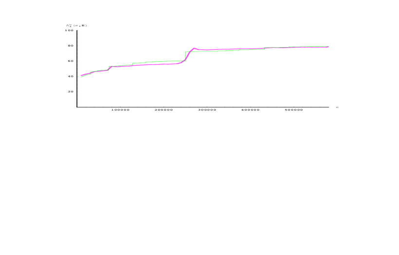
Figure 1: $\overline{\Delta}_{3}^{\infty}\left(\epsilon;E\right)$ vs. $\epsilon$ for $\beta=3\times 10^{6}$. The thicker line is the numerical simulation while the thinner line is the analytical result given by eq. (69), with modification (71).

While (69) provides a wonderful fit to numerical data on the top plateau, it predicts much bigger jumps between the plateaus than is seen numerically. As a results, to fit lower plateaus we empirically added an appropriate empirical constant via substitution

$$\left[\frac{M_{r}}{\gamma^{(cir)}}\right]\rightarrow\left[\frac{M_{r}}{\gamma^{(cir)}}\right]+\sum_{n=1}^{\left[M_{r}/\gamma^{(cir)}\right]-1}\frac{1}{2^{2n-1}}$$ (71)

At this time we do not have a good explanation for this discrepancy. Further, the theoretical formula predicts additional noticeable jump further up in the spectrum, when $\gamma^{(cir)}=3/2$, which is not seen on the experimental curve.

With the same modification (71) in eq. (70), we plot $\Sigma^{\infty}\left(\epsilon;E\right)$ as a function of $E$ for two different values of $\epsilon$

Figure 2: $\Sigma^{\infty}\left(\epsilon;E\right)$ vs. $E$ for $\beta=3\times 10^{6}$ and $\epsilon=5\times 10^{5}$. The thicker line is the numerical simulation while the thinner line is the analytical result given by eq. (70), with modification (71) (for this value of $\epsilon$, the correction is actually zero, as explained in text).

Figure 3: Same as Fig. (2) for $\epsilon=2\times 10^{5}$.

Clearly, while the periodicity is superbly predicted by the analytical expression, there is a striking difference in the intermediate structure in comparison with the numerical results.

VII Conclusions

We predict analytically, and observe numerically, quantum Hall like jumps of the averaged saturation level rigidity in a modified Coulomb problem. These are explained semiclassically in terms of jumps in the winding numbers of the shortest periodic orbits as the position of the interval center moves through the energy spectrum. Also, analytically and numerically, we predict sinusoidal oscillations of the saturation level number variance with the interval width. This is a striking result which indicates that while distribution of the levels on a interval varies greatly from sample to sample, the total number of levels in the interval may be nearly identical for certain values of the interval width. This is because all the higher harmonics are integer fractions of the shortest periodic orbit and add up coherently. The latter explains the difference with other systems, such as rectangular box, where the oscillations may be large but the variance doesn’t reach a near-zero value.

Appendix A Amplitudes of periodic orbits

The amplitude of an irreducible cycle $\mathbf{M}=\left\{M_{1},M_{2}\right\}$ is given byBT

$$A_{\mathbf{M}}^{2} =\frac{2\pi}{T_{\mathbf{M}}^{2}\left|\boldsymbol{\omega}\cdot\partial\mathbf{I}_{\mathbf{M}}/\partial T_{\mathbf{M}}\det\left\{\partial\omega_{i}/\partial I_{k}\right\}_{\mathbf{M}}\right|}$$ (72)

$$\boldsymbol{\omega}\left(\mathbf{I}_{\mathbf{M}}\right)T_{\mathbf{M}} =2\pi\mathbf{M}$$ (73)

This equation can be simplified by differentiating (73) on $T$, which gives

$$T\sum_{j=1}^{2}\frac{\partial\omega_{i}}{\partial I_{j}}\frac{\partial I_{j}}{\partial T}+\omega_{i}=0$$ (74)

whereof

$$\boldsymbol{\omega}\cdot\partial\mathbf{I}/\partial T=\frac{-\left[\omega_{1}^{2}\left(\partial\omega_{2}/\partial I_{2}\right)+\omega_{2}^{2}\left(\partial\omega_{1}/\partial I_{1}\right)\right]+\omega_{1}\omega_{2}\left(\partial\omega_{1}/\partial I_{2}+\partial\omega_{2}/\partial I_{1}\right)}{T\det\left\{\partial\omega_{i}/\partial I_{k}\right\}}$$ (75)

so that

$$A_{\mathbf{M}}^{2}=\frac{2\pi}{T_{\mathbf{M}}\left|-\left[\omega_{1}^{2}\left(\partial\omega_{2}/\partial I_{2}\right)+\omega_{2}^{2}\left(\partial\omega_{1}/\partial I_{1}\right)\right]+\omega_{1}\omega_{2}\left(\partial\omega_{1}/\partial I_{2}+\partial\omega_{2}/\partial I_{1}\right)\right|_{\mathbf{M}}}$$ (76)

which shows a universal dependence of $A_{\mathbf{M}}^{2}$ on $T_{\mathbf{M}}$.

Here, $\mathbf{I=}\left\{I_{r},I_{\theta}\right\}$ and $\boldsymbol{\omega}\mathbf{=}\left\{\omega_{r},\omega_{\theta}\right\}=\nabla_{\mathbf{I}}\epsilon\left(\mathbf{I}\right)$, where $\epsilon$ is given by (59). Consequently, from (76), we find

$$A_{\mathbf{M}}^{2}=\frac{2\pi}{3\epsilon T_{\mathbf{M}}}=\frac{\omega_{r}}{3\epsilon M_{r}}$$

where $\omega_{r}$ is given by (60).

References

• (1) J. M. A. S. P. Wickramasinghe, B. Goodman, and R. A. Serota, Phys. Rev. E72,056209 (2005).
• (2) Martin C. Gutzwiller ”Chaos In Classical And Quantum Mechanics” (Springer-Verlag, New York, 1990).
• (3) M. V. Berry, Proc. R. Soc. Lond. A400, 229 (1985).
• (4) G. Casati, B. V. Chirikov and I. Guarneri, Phys. Rev. Lett. 54, 1350 (1985).
• (5) P. M. Bleher and J. L. Lebowitz, J. Stat. Phys. 74, 167 (1993).
• (6) Felix von Oppen, Phys. Rev. B50, 17151 (1994).
• (7) T. A. Brody, J. Flores, J. B. French, P. A. Mello, A. Pandey, and S. S. M. Wong, Rev. Mod. Phys. 53, 385 (1981).
• (8) Konstantin Efetov ”Supersymmetry In Disorder And Chaos” (Cambridge University Press, 1997).
• (9) G. L. Kotkin and V. G. Serbo, ”Collection Of Problems In Classical Mechanics” (Pergamon Press, 1971).
• (10) L. D. Landau and E. M. Lifshitz, ”Mechanics” (Pergamon Press, 1988).
• (11) L. D. Landau and E. M. Lifshitz, ”Quantum Mechanics” (Pergamon Press, 1981).
• (12) M. V. Berry and M. Tabor, J. Phys. A10, 371 (1977).
• (13) E. Weisstein, ”Clausen Function,” $<$http://mathworld.wolfram.com/ClausenFunction.html$>$.