Control momentum entanglement with atomic spontaneously generated coherence

Abstract

With atomic spontaneously generated coherence (SGC), we propose a novel scheme to coherently control the atom–photon momentum entanglement through atomic internal coherence. A novel phenomena of “phase entanglement in momentum” is proposed, and we found, under certain conditions, that super–high degree of momentum entanglement can be produced with this scheme.

.

I Introduction

Entanglement with continuous variable attracts many attentions for its fundamental importance in quantum nonlocality EPR and quantum information science and technology rmp . As a physical realization, the continuous momentum entanglement between atom and photon has been extensively studied in recent years Singlephoton ; 3-D spontaneous ; scattering ; GR ; exp . In the process of spontaneous emission Singlephoton ; 3-D spontaneous , the momentum conservation will induce the atom–photon entanglement, with its degree inversely proportional to the linewidth of the emission. Therefore, by squeezing the effective transition linewidth, super–high degree of momentum entanglement may be produced scattering ; GR . With this entanglement, further, it is possible to realize the best localized single–photon wavefunction even in free space Singlephoton .

In this paper, we propose a novel scheme to coherently control and enhance the momentum entanglement between single atom and photon. We found, for the atomic system with spontaneously generated coherence (SGC) SGC ; atomic coherence contr , that the interference between photons emitted along different quantum pathways could enhance the momentum entanglement significantly. Due to SGC, the degree of entanglement is determined by the intensity of the interference in the emission process, and can be effectively controlled by the atomic coherence between its internal states. Under this new mechanism of entanglement enhancement, the entangled system could exhibit novel feature of “phase entanglement” in the momentum space, which does not exist in the previous schemes without interference Singlephoton ; 3-D spontaneous ; scattering ; GR ; exp ; and the degree of entanglement is found to be “abnormally” proportional to the atomic linewidth. Moreover, by effectively squeezing the separation of the upper levels, it is possible to produce super–high degree of momentum entanglement for the atom–photon system with this scheme GR-disentanglement .

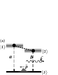
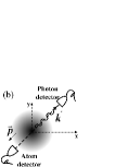
Figure 1: (a) The atom has two closely–lying upper levels to provide different quantum pathways for the spontaneous emission. The momentum conservation makes the emitted photon entangled with the recoiled atom. (b) Schematic diagram for the detections. The two detectors are fixed in one dimension as in the reported experiments exp .

II Theoretical model

As shown in Fig. 1 (a), the atom with two nearly–degenerate upper levels has two transition pathways (denoted by “a” and “b” respectively) to induce the momentum entanglement with the emitted photon. To have strong interference between the two transitions, we assume that the dipoles $\mu_{a,b}$ for the transitions are parallel with each other SGC . Then, the Hamiltonian under the rotating wave approximation (RWA) can be written as:

$$\hat{H} = \frac{(\hbar\hat{\vec{p}})^{2}}{2m}+\sum_{\vec{k}}\hbar\omega_{\vec{k}}\hat{a}^{{\dagger}}_{\vec{k}}\hat{a}_{\vec{k}}+\hbar\omega_{a}\hat{\sigma}_{11}+\hbar\omega_{b}\hat{\sigma}_{22}$$

$$+ \hbar\sum_{\vec{k}}\left[g_{a}(\vec{k})\hat{\sigma}_{31}\hat{a}^{{\dagger}}_{\vec{k}}e^{-i\vec{k}\cdot\vec{r}}+g_{b}(\vec{k})\hat{\sigma}_{32}\hat{a}^{{\dagger}}_{\vec{k}}e^{-i\vec{k}\cdot\vec{r}}+{\rm H.c.}\right],$$

where $\hbar\hat{\vec{p}}$ and $\vec{r}$ denote atomic center–of–mass momentum and position operators, $\hat{\sigma}_{ij}$ the atomic operator $|i\rangle\langle j|$ ($i,j=1,2,3$), and $\hat{a}_{\vec{k}}$ ($\hat{a}^{{\dagger}}_{\vec{k}}$) is the annihilation (creation) operator for the $k$th vacuum mode with wave vector $\vec{k}$ and frequency $\omega_{\vec{k}}\equiv ck$. $g_{a,b}(\vec{k})$ are the coupling coefficients for the transitions “a” and “b”, where we use $\vec{k}$ to denote both the momentum and polarization of the vacuum mode for simplicity.

With the spontaneous emission, the momentum conservation will make the emitted photon entangled with the recoiled atom in momentum. It is convenient to depict this entangling process in the Schrödinger picture, and expand the photon–atom state as:

$$|\psi\rangle = \sum_{\vec{q}}C_{1}(\vec{q},t)|\vec{q},0,1\rangle+\sum_{\vec{q}}C_{2}(\vec{q},t)|\vec{q},0,2\rangle$$ (2)

$$+ \sum_{\vec{q},\vec{k}}C_{3}(\vec{q},\vec{k},t)|\vec{q},1_{\vec{k}},3\rangle\ ,$$

where the arguments in the kets denote, respectively, the wave vector of the atom, the photon, and the atomic internal states.

With the transformation

$$C_{1,2}(\vec{q},t) = \exp\left[-i\left(\frac{\hbar q^{2}}{2m}+\omega_{a}\right)t\right]\cdot A_{1,2}(\vec{q},t)\ ,$$ (3)

$$C_{3}(\vec{q},\vec{k},t) = \exp\left[-i\left(\frac{\hbar q^{2}}{2m}+ck\right)t\right]\cdot B(\vec{q},\vec{k},t)\ ,$$ (4)

and Weisskopf–Wigner approximation, we yield the dynamic equations from the Schrödinger equation:

$$\frac{{\rm d}A_{1,2}(\vec{q},t)}{{\rm d}t} = -\frac{\gamma_{a,b}}{2}A_{1,2}(\vec{q},t)$$ (5)

$$- \frac{\varepsilon\sqrt{\gamma_{a}\gamma_{b}}}{2}A_{2,1}(\vec{q},t)e^{\pm i(\omega_{a}-\omega_{b})t},$$

$$i\frac{{\rm d}B(\vec{q},\vec{k})}{{\rm d}t} = g_{a}(\vec{k})e^{i[-\hbar(2\vec{q}+\vec{k})\cdot\vec{k}/2m+ck-\omega_{a}]t}A_{1}(\vec{q}+\vec{k})$$

$$+ g_{b}(\vec{k})e^{i[-\hbar(2\vec{q}+\vec{k})\cdot\vec{k}/2m+ck-\omega_{b}]t}A_{2}(\vec{q}+\vec{k})\ ,$$

where the nonrelativistic approximation ($\hbar\vec{q},\ \hbar\vec{k}\ll mc$) and the relation $\omega_{12}\equiv\omega_{a}-\omega_{b}\ll\omega_{a},\omega_{b}$ are used. $\gamma_{a,b}=2\pi\sum_{\vec{k}}|g_{a,b}(\vec{k})|^{2}\delta[\hbar(2\vec{q}-\vec{k})\cdot\vec{k}/2m+\omega_{a,b}-ck]$ are the linewidthes for the two transitions, and $\varepsilon\equiv\vec{\mu}_{a}\cdot\vec{\mu}_{b}/|\vec{\mu}_{a}|\cdot|\vec{\mu}_{b}|=1$ as we have assumed previously. Suppose the atom is initially prepared to a superposed state $A_{10}|1\rangle+A_{20}|2\rangle$ and has a Gaussian wavepacket as $G(\vec{q})\propto e^{-(\vec{q}/\delta q)^{2}}$, and the detections are restricted in one dimension as in Fig. 1 (b), the one–dimensional steady solutions for Eqs. (5) and (6) yield:

$$A_{1}(q,t\rightarrow\infty)=A_{2}(q,t\rightarrow\infty)=0\ ,$$ (7)

$$B(q,k,t\rightarrow\infty)=-i\chi_{0}\exp[-(\Delta q/\eta)^{2}]\times$$ (8)

$$\left[\frac{C_{1}(2g_{b}s_{1}/\varepsilon\sqrt{\gamma_{a}\gamma_{b}}-g_{a})}{i(\Delta q+\Delta k)+(\frac{s_{1}}{\gamma_{a}}-\frac{1}{2})}+\frac{C_{2}(2g_{b}s_{2}/\varepsilon\sqrt{\gamma_{a}\gamma_{b}}-g_{a})}{i(\Delta q+\Delta k)+(\frac{s_{2}}{\gamma_{a}}-\frac{1}{2})}\right],$$

where the parameters are defined as:

$$s_{1,2}\equiv\frac{1}{2}(\lambda\pm\sqrt{\lambda^{2}+\varepsilon^{2}\gamma_{a}\gamma_{b}})\ ,$$ (9)

$$\lambda\equiv\frac{1}{2}(\gamma_{a}-\gamma_{b})+i\omega_{12}\ ,$$ (10)

$$C_{1,2}\equiv\pm\frac{s_{2,1}A_{10}+\frac{1}{2}\varepsilon\sqrt{\gamma_{a}\gamma_{b}}A_{20}}{s_{2}-s_{1}}\ ,$$ (11)

$$\eta\equiv\frac{\delta q\hbar k_{0}}{m\gamma_{a}}\ ,\ \ \ \ \ \ \ k_{0}\equiv\frac{\omega_{a}}{c}\ ,$$ (12)

and the effective wave vectors are defined by:

$$\Delta k \equiv \frac{k-k_{0}}{\gamma_{a}/c}\ ,\ \ \ \ \ \Delta q\equiv\frac{\hbar k_{0}}{m\gamma_{a}}(q-k_{0})\ ,$$ (13)

where $\chi_{0}$ is the normalized coefficient.

III amplitude entanglement in momentum

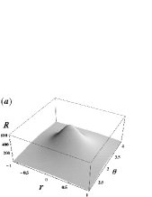
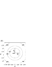
Figure 2: (a) The “amplitude entanglement” $R$ ratio is plotted in dependence on the atomic coherence $r$ and $\theta$ with $\delta=0.02$, $\eta=0.1$. (b) The contour plot of figure (a). The circular contours indicates the symmetric roles played by $r$ and $\theta$ in controlling the $R$ ratio. The FWHM is denoted with $\delta_{\theta}$ and $\delta_{r}$ as in the figure.

The nonfactorization of the wavefunction in Eq. (8) indicates the entanglement of the atom–photon system. In both theoretical 3-D spontaneous ; photoionization and experimental exp studies of the continuous entanglement, the ratio (denoted by “$R$”) of the conditional and unconditional variances plays a central role, since it is a straightforward experimental measure of the nonseparability, i.e., the entanglement, of the system.

With the single–particle measurement, the unconditional variance for the effective momentum of the atom is $\delta q^{{\rm single}}\equiv\langle\Delta q^{2}\rangle-\langle\Delta q\rangle^{2}$, where the average $\langle\cdot\rangle$ is taken over the whole ensemble (cf. Eq. (24)). Meanwhile, the coincidence measurement gives the conditional variance as $\delta q^{{\rm coin}}\equiv\langle\Delta q^{2}\rangle_{\Delta k_{0}}-\langle\Delta q\rangle^{2}_{\Delta k_{0}}$, where the photon is now assumed to be detected at some known $\Delta k_{0}$ (cf. Eq. (25)). With the two variances, we have:

$$R\equiv\delta q^{{\rm single}}/\delta q^{{\rm coin}}\geq 1.$$ (14)

Since the $R$ ratio is constructed from the amplitude information of the wavefunction, it evaluates the “amplitude entanglement” for the system; and as it is defined for the momentum measurements, its value does not vary with time 3-D spontaneous ; phase entang. and can be directly detected in experiments exp .

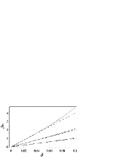
Figure 3: The FWHM of the $R$ ratio is plotted in solid lines in dependence on $\delta$ with $\eta=0.05,0.1,0.2$ from the top to the bottom. Dashed lines are the fitted function $2\delta/\eta$.

Due to the interference with the transitions, the $R$ ratio highly depends on the initial coherence of the two upper levels, which can be described with a couple of parameters $(r,\theta)$ defined as $e^{r+i\theta}=A_{10}/A_{20}$, where $r$ controls the relative occupation probabilities for the two upper levels, and $\theta$ determines their coherent phase. In further discussions, we assume $\gamma_{1}=\gamma_{2}\equiv\gamma$ for simplicity, and define a dimensionless small parameter $\delta\equiv\omega_{12}/\gamma<1$ since the upper levels are nearly degenerate.

With Eqs. (8) and (14), we get the relations between $R$ and the coherence parameters $r$ and $\theta$ as in Fig. 2. Under the conditions $\eta\ll 1$ and $\delta^{2}/\eta\ll 1$ explanations , we find that the function $R(r,\theta)$ can be well approximated by a Lorentzian shape, and as shown in Fig. 2 (b), the parameters $r$ and $\theta$ play very symmetric roles in controlling the “amplitude entanglement” $R$, although they are defined with quite different physical essence.

With the above approximations, we find that the $R$ ratio is maximized at the “dark state coherence”, i.e.,

$$R_{{\rm max}}=R(r=0,\theta=\pi)\approx\frac{\sqrt{2\pi}\eta}{\delta^{2}},$$ (15)

whereas $r=0$ and $\theta=0$ minimizes the value of $R$. Furthermore, the full width at half maximum (FWHM) of the function $R(r,\theta)$ can be well approximated by:

$$\delta_{r}\approx\delta_{\theta}\approx\frac{2\delta}{\eta},$$ (16)

as shown in Fig. 3. Therefore, with properly chosen atomic parameters $\eta$ and $\delta$, this scheme could be used to produce significant “amplitude entanglement” in a relatively large range of the atomic coherence. For example, with $\eta=\delta=0.01$, the “amplitude entanglement” of $R>100$ can be produced within the range of $0.018<|A_{10}/A_{20}|^{2}<55$, and $0.36\pi<\theta<1.6\pi$.

IV full entanglement and steady phase entanglement in momentum

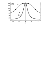
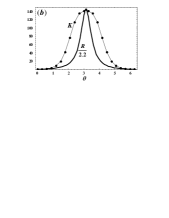
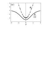
Figure 4: Plots of $K$ and $R/2.2$ in dependence on the atomic coherence $r$ or $\theta$. (a) $\eta=0.2$, $\delta=0.04$, $\theta$ is fixed at $\pi$. (b) $\eta=0.2$, $\delta=0.04$, $r$ is fixed at $0$. (c) $\eta=0.5$, $\delta=0.08$, $\theta$ is fixed at $0$.

In order to evaluate the full entanglement for the bipartite system in a pure state, one may use the “Schmidt number”Singlephoton ; Parametric Down Conversion . With the method of Schmidt decomposition Schmidt num , the entangled wavefunction can be uniquely converted into a discrete sum as:

$$B(q,k)=\sum_{n}\sqrt{\lambda_{n}}\psi_{n}(q)\phi_{n}(k),$$ (17)

where the $\lambda_{n}$’s are ordered as $\lambda_{1}\geq\lambda_{2}\geq\lambda_{3}\geq...$ and the $\psi_{n}(q)$’s and $\phi_{n}(k)$’s are complete orthonormal sets for the Hilbert spaces of the atom and the photon, respectively. With Eq. (17), the Schmidt number $K$ is defined as:

$$K\equiv\frac{1}{\sum_{n}\lambda_{n}^{2}}\geq 1.$$ (18)

As the Schmidt number is constructed with full information of the wavefunction, and is invariant under representation transformations, it represents the full entanglement information for the entangled system.

We plot the numerical results of $K$ in comparison with the $R$ ratio in Fig. 4, where one sees that, both of them are maximized at the coherence of $(r=0,\theta=\pi)$ and minimized at $(r=0,\theta=0)$. However, compared with $R(r,\theta)$, $K(r,\theta)$ has a much slower decay around its maximum, which indicates that, by tuning the atomic coherence, more entanglement may be transferred into the phase and can no longer be observed by the amplitude detection with the $R$ ratio. Actually, due to the “phase entanglement”, the systems with the same Schmidt number may exhibit significantly different “amplitude entanglement” under different initial conditions. For example, with parameters $\delta=0.04,\eta=0.7,r=0,\theta=\pi$, for the system we have $K\approx 490$ and $R\approx 1200$; however, when the initial conditions change to $\eta^{\prime}=1,r^{\prime}=0.4$, the system has the same Schmidt number $K^{\prime}=K\approx 490$ but a significantly smaller “amplitude entanglement” $R^{\prime}\approx 96\approx 0.08R$, because more entanglement information is transferred into the phase.

Similar phenomenon of the “phase entanglement” has been reported recently 3-D spontaneous ; photoionization ; phase entang. in the position space. Due to the spreading of the wavepacket, the phase entanglement in position space appears only in a short time interval and must be detected by a series of spatial measurements in time photoionization . However, in this scheme, as the phase entanglement is in the momentum space, it is not affected by the wavepacket’s spreading and keeps invariant with time, therefore, it will be much easier to be observed in experiments with direct detections exp .

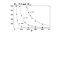
Figure 5: The numerical results of $K$ (in spots) and the function $R/2.2$ (in solid line) are plotted at the maximum atomic coherence $r=0$ and $\theta=\pi$.

By comparing with the “maximally entangled states”, it is possible to formally evaluate the “phase entanglement” for all the states under this scheme. For the states with entanglement maximized by $r$ and $\theta$, the wavefunctions take the form:

$$B(q,k,t\rightarrow\infty)\approx\frac{\chi_{0}\cdot e^{-(\Delta q/\eta)^{2}}}{i(\Delta q+\Delta k)-\delta^{2}/4}\ ,$$ (19)

and then the Schmidt number can be well approximated as Singlephoton ; scattering :

$$K_{{\rm max}}\approx 1+0.28(4\eta/\delta^{2}-1).$$ (20)

With Eqs. (20) and (15), we have:

$$K_{{\rm max}} =K(r=0,\theta=\pi)\approx\frac{R_{{\rm max}}}{2.2}\ ,$$ (22)

$$\approx\frac{1.12\hbar k_{0}\delta q\gamma}{m\omega_{12}^{2}}.$$

As shown in Fig. 5, the relation of Eq. (21) is well fulfilled for all $\eta$ and $\delta$ with $\eta/\delta^{2}\gg 1$ and $\eta\ll 1$ explanations .

The linear relation between $K_{{\rm max}}$ and $R_{{\rm max}}$ in Eq. (21) indicates that there is little phase entanglement for the “maximally entangled states” produced with $r=0$ and $\theta=\pi$, since their full entanglement can be completely obtained by the amplitude detection with the $R$ ratio. For states with other $r$ and $\theta$, as in Fig. 4, we always have $K\geq R/2.2$, therefore, the phase entanglement can be evaluated by:

$$PE\equiv\frac{2.2K}{R}\geq 1.$$ (23)

The quantity $PE$, as we stated above, evaluates the degree of the “phase entanglement” for all the states produced with the control parameter $\eta$, $\delta$, $r$ and $\theta$ under this scheme.

In the previous works on atom–photon momentum entanglement Singlephoton ; 3-D spontaneous ; scattering ; GR , the entanglement is produced along a single quantum pathway without interference. Therefore, the system has a similar wavefunction as Eq. (19) and exhibits little “phase entanglement” in momentum as we explained above. In this scheme, the interference between two quantum pathways produce obviously different entangled state as in Eq. (8), which may give rise to the significant “phase entanglement” in the momentum space.

Moreover, for the single–path scheme Singlephoton ; 3-D spontaneous ; scattering ; GR , the Schmidt number is always inversely proportional to the linewidth of the transition; while in our proposed scheme, however, one sees that $K_{{\rm max}}\propto\gamma$ as in Eq. (22). This abnormal phenomenon indicates that the mechanism for the entanglement in this scheme is essentially different with the previous ones Singlephoton ; 3-D spontaneous ; scattering ; GR . By squeezing the effective separation of the upper levels, as $K\propto 1/\omega_{12}^{2}$ in Eq. (22), it is possible to use this scheme to produce supper–high degree of momentum entanglement for the atom–photon systems GR-disentanglement .

V Schmidt modes

Figure 6: First three Schmidt modes are compared between states $B(q,k)$ and $B^{\prime}(q,k)$ with $\delta=0.1$, $\eta=0.94$, $r=0$, $\theta=\pi$ and $\delta^{\prime}=\delta$, $\theta^{\prime}=\theta$, $\eta^{\prime}=1$, $r^{\prime}=-0.4$, respectively, where one has $K^{\prime}\approx K$ and $R^{\prime}\approx 0.3R$. The phase entanglement of $B^{\prime}(q,k)$ broadens the fist Schmidt mode and decreases the number of peaks for the rest ones. The inset shows the distribution of the eigenvalues $\lambda_{n}$ in the Schmidt decomposition.

The phenomenon of “phase entanglement” is related to the coherence between different Schmidt modes $\psi_{n}(q)$ defined in Eq. (17). With the Schmidt decomposition, the unconditional variance $\delta q^{{\rm single}}$ can be written as:

$$\delta q^{{\rm single}} = \int{\rm d}\Delta q\ {\rm d}\Delta k\Delta q^{2}|B(q,k)|^{2},$$ (24)

$$= \int{\rm d}\Delta q\ \Delta q^{2}\sum_{n}\lambda_{n}|\psi_{n}(q)|^{2},$$

$$= \int{\rm d}\Delta q\ \Delta q^{2}E_{{\rm i}}(q),$$

where $E_{{\rm i}}(q)\equiv\sum_{n}\lambda_{n}|\psi_{n}(q)|^{2}$ is a probability distribution constructed by an “incoherent” summation of different Schmidt modes weighed by $\lambda_{n}$. The conditional variance, however, is written as:

$$\delta q^{{\rm coin}}=\frac{1}{N}\int{\rm d}\Delta q\ \Delta q^{2}|B(q,\Delta k_{0})|^{2},$$

$$=\frac{1}{N}\int{\rm d}\Delta q\ \Delta q^{2}|\sum_{n}\sqrt{\lambda_{n}}\phi_{n}(\Delta k_{0})\psi_{n}(q)|^{2},$$ (25)

where $N=\sum_{n}\lambda_{n}|\phi_{n}(\Delta k_{0})|^{2}$ is the normalized coefficient. When $K$ is large, $\phi_{n}(\Delta k_{0})$ can be approximated as a constant, then we have:

$$\delta q^{{\rm coin}}\approx\int{\rm d}\Delta q\ \Delta q^{2}|E_{{\rm c}}(q)|^{2},$$ (26)

where $E_{{\rm c}}(q)\equiv\sum_{n}\sqrt{\lambda_{n}}\psi_{n}(q)$ is a “coherent superposition” of different Schmidt modes. Comparing Eq. (24) with (26), one sees that the $R$ ratio defined as $R=\delta q^{{\rm single}}/\delta q^{{\rm coin}}$ actually represents the degree of the packet narrowing caused by the coherence between different Schmidt modes.

In Fig. 6, we compare the atomic Schmidt modes between two states $B(q,k)$ and $B^{\prime}(q,k)$ with $K^{\prime}\approx K$ and $R^{\prime}\approx 0.3R$. It is found that the phase entanglement will significantly broaden the fist few Schmidt modes and decrease the number of peaks for the rest ones. Moreover, the coherence between different Schmidt modes diminishes, which decreases the $R$ ratio as we stated above.

The photonic Schmidt modes exhibit similar properties as the atomic modes. We emphasize that the property of Gaussian localization Singlephoton ; scattering of the single–photon modes still remains in spite of the shape distortions caused by the interference. Therefore, it demonstrates the possibilty to apply the idea of “localized single–photon wavefunction in free space”Singlephoton to even more complicated atomic systems.

VI conclusion

In summary, we have investigated the recoiled–induced atom–photon entanglement in the atomic system with SGC. Due to the quantum interference in the emission process, the momentum entanglement can be effectively controlled by the atomic internal coherence, and may be greatly enhanced by increasing the linewidth or squeezing the separation of the upper levels as in Eq. (22). The novel phenomenon of “momentum phase entanglement” is shown and evaluated quantitively. Further, we compare the atomic Schmidt modes for different entangled states in the momentum space.

In order to experimentally observe these phenomena, one needs two nearly degenerate upper levels with parallel dipole moments. This configuration has been extensively studied both theoretically and experimentally SGC ; atomic coherence contr in recent years, and can be realized by mixing different parity levels or by using dressed-state ideas. With proper control of the atomic coherence atomic coherence contr , it is most probable to observe the “momentum phase entanglement” in experiments. Furthermore, by squeezing the separation of the upper-levels in dressed–state with an auxiliary light SGC , this scheme can be used to produce super-high degree of entanglement for realistic applications GR-disentanglement .

This work is supported by the National Natural Science Foundation of China (Grant No. 10474004), and DAAD exchange program: D/05/06972 Projektbezogener Personenaustausch mit China (Germany/China Joint Research Program).

References

- (1) A. Einstein, B. Podolsky, N. Rosen, Phys. Rev. 47, 777 (1935); J. C. Howell et. al., Phys. Rev. Lett. 92, 210403 (2004).
- (2) S. L. Braunstein and P. V. Loock, Rev. Mod. Phys. 77, 513 (2005).
- (3) K. W. Chan, C. K. Law, and J. H. Eberly, Phys. Rev. Lett. 88, 100402 (2002).
- (4) M. V. Fedorov et. al., Phys. Rev. A 72, 032110 (2005).
- (5) K. W. Chan et. al., Phys. Rev. A 68, 022110 (2003); J. H. Eberly, K. W. Chan and C. K. Law, Phil. Trans. R. Soc. Lond. A 361, 1519 (2003).
- (6) R. Guo and H. Guo, Phys. Rev. A 73, 012103 (2006).
- (7) M. D. Reid and P. D. Drummond, Phys. Rev. Lett. 60, 2731 (1988); Michael S. Chapman et al., Phys. Rev. Lett. 75, 3783 (1995); Christian Kurtsiefer et al., Phys. Rev. A 55, R2539 (1997).
- (8) S. Y. Zhu and M. O. Scully, Phys. Rev. Lett 76, 388 (1996); H. R. Xia, C. Y. Ye, and S. Y. Zhu, Phys. Rev. Lett. 77, 1032 (1996).
- (9) M. O. Scully, S. Y. Zhu and A. Gavrielides, Phys. Rev. Lett. 62, 2813 (1989); S. Y. Zhu, R. C. F. Chan and C. P. Lee, Phys. Rev. A 52, 710 (1995).
- (10) arXiv: R. Guo and H. Guo, quant–ph/0611205.
- (11) M. V. Fedorov et al., Phys. Rev. A 69, 052117 (2004).
- (12) arXiv: K. W. Chan and J. H. Eberly, quant–ph/0404093.
- (13) In typical atomic system, is of order or smaller, e.g., for sodium one has ; moreover, the condition is equivalent to , which is our major concern.
- (14) C. K. Law, I. A. Walmsley, and J. H. Eberly, Phys. Rev. Lett. 84, 5304 (2000); C. K. Law and J. H. Eberly, Phys. Rev. Lett. 92, 127903 (2004).
- (15) R. Grobe et al., J. Phys. B 27, L503 (1994); S. Parker et al., Phys. Rev. A 61, 032305 (2000).